Dynamic Factor Model with infinite-dimensional
factor space: Forecasting
Mario
Forni
, Alessandro
Giovannelli
, Marco
Lippi
,
Stefano
Soccorsi
∗April 12, 2018
Abstract. The paper compares the pseudo real-time forecasting performance of three
Dynamic Factor Models: (i) The standard principal-component model introduced by Stock and Watson in 2002, (ii) The model based on generalized principal components, introduced by Forni, Hallin, Lippi and Reichlin in 2005, (iii) The model recently proposed by Forni, Hallin, Lippi and Zaffaroni in 2015. We employ a large monthly dataset of macroeconomic and financial time series for the U.S. economy, which includes the Great Moderation, the Great Recession and the subsequent recovery (an update of the so-called Stock and Watson dataset). Using a rolling window for estimation and prediction, we find that (iii) significantly outperforms (i) and (ii) in the Great Moderation period for both Industrial Production and Inflation, that (iii) is also the best method for Inflation over the full sample. However, (iii) is outperformed by (ii) and (i) over the full sample for Industrial Production.
Keywords: Time Series Forecasting, Macroeconomic Forecasting, Dynamic Fac-tor Models.
∗Forni: Universit`a di Modena e Reggio Emilia, Modena, Italy, CEPR and RECent. Giovannelli:
Universit`a di Roma Tor Vergata, Roma, Italy. Lippi (Corresponding author) Einaudi Institute for
Economics and Finance, Via Sallustiana 62, 00187 Roma, Italy. Email: [email protected]. Soccorsi: Lancaster University Management School, Lancaster, UK. We are grateful for very useful suggestions to Donatella Albano, Manfred Deistler, Fabio Della Marra, Domenico Giannone, Jean-Paul L’Huillier and two anonymous referees. The contribution of the Italian Ministry of Education, University and Research for the PRIN project 2010J3LZEN 003 is gratefully acknowledged.
1
Introduction
This paper compares the pseudo real-time forecasting performance of three Large-Dimensional Dynamic Factor Models for the US monthly macroeconomic dataset over the period February 1985 to August 2014, this including the so-called Great Moderation and the Great Recession.
Large-Dimensional Dynamic Factor Models represent each variable in the dataset
as decomposed into a common component, driven by a small (as compared to the
number of series in the dataset) and fixed (as the number of series grows) number of common factors and an idiosyncratic component. The latter are assumed to be orthogonal across different variables or only weakly correlated, so that the covariance of the variables is mostly accounted for by the common components. Typically, the asymptotic results are obtained for n, the number of series, and T, the number of observations for each series, both tending to infinity. Among the different versions of the Dynamic Factor Model we selected:
(i) SW. The model introduced in Stock and Watson (2002a,b). The factors are estimated by means of the standard Principal Components of the variables in the dataset. The forecast of the variable of interest, call it yt, is obtained by
regressing yt+h on the factors and the variable yt, plus possibly lags of the
factors and yt.
(ii) FHLR. A variant of the previous model which has been proposed in Forni et al. (2005). In a first step the covariances of the common and the idiosyncratic com-ponents are estimated using a frequency-domain method introduced in Forni et al. (2000). In the second step such covariances are employed to estimate the factors by means of Generalized Principal Components.
(iii) FHLZ. Both models (i) and (ii) assume that the space spanned by the common components at any time t stays finite-dimensional as n tends to infinity. In two recent papers, Forni et al. (2015, 2017), it is assumed that a finite num-ber of common shocks drive the common components, though the common components themselves are allowed to span an infinite-dimensional space. The
dynamic relationship between the variables and the factors in this model is more general as compared to (i) and (ii). However, its estimation is rather complex and no systematic comparison with (i) and (ii) has as yet been produced. The literature comparing SW and FHLR has reached mixed conclusions so far. Using the monthly U.S. macroeconomic dataset known as the Stock and Watson dataset, Boivin and Ng (2005) found that SW generally outperforms FHLR, whereas D’Agostino and Giannone (2012) found the two methods to perform equally well in their sample, even if different performances are found in subsamples. In particular, FHLR fares better during the Great Moderation, consistently with the results in the present paper. Schumacher (2007), using German data, finds that FHLR provides more accurate forecasts of the GDP. A similar result is obtained in den Reijer (2005) with Dutch macroeconomic data.
In the present paper we extend the comparisons in Boivin and Ng (2005) and D’Agostino and Giannone (2012) to an update of the Stock and Watson dataset, and include the new FHLZ forecasting model. Our dataset starts in January 1959 and end in August 2014, thus including the Great Moderation, the Great Recession and the subsequent recovery.
The main task of the paper is evaluating the performance of the new model FHLZ with respect to SW, the standard in this literature, and FHLR, which shares with FHLZ the frequency domain approach. Important variants of the Dynamic
Factor Model such as e.g. Pe˜na and Poncela (2004), Kapetanios and Marcellino
(2009) are not considered (for wider comparisons of forecast results with Dynamic Factor Models, see Schumacher (2007) and Eickmeier and Ziegler (2008)). Rather, we compare FHLZ, FHLR and SW with (1) two “second-generation” factor models, namely Doz et al. (2011), in which a maximum likelihood estimation method of the factors is introduced, and the three-pass regression filter of Kelly and Pruitt (2015), (2) a model based on Bayesian shrinkage, De Mol et al. (2008).
A distinctive feature of our exercise is that we use a fairly large subsample, February 1960 to December 1984, to calibrate the models. In particular, how to determine the number of factors in SW and FHLR, the number of lags of the factors
or of the variable to be predicted, the Kernel in the spectral estimation for FHLR and FHLZ, etc. The selected models are then run and compared in the remaining sample, January 1985 to August 2014, which makes the present paper the first to provide a thorough comparison of different factor models over the Great Moderation, the Great Recession and the subsequent recovery.
Our main results are:
(I) In the Great Moderation period, where the assumption of stationarity of the series in the dataset (after suitable transformations) underlying all factor mod-els is by and large fulfilled, FHLZ significantly outperforms FHLR, SW and AR both for Industrial Production and Inflation.
(II) In the full sample, including the Great Recession and the subsequent recovery, FHLZ remains the best method for CPI, albeit slightly, whereas FHLR and SW outperform FHLZ and AR for Industrial Production.
(III) We also run forecasts for all single series in the dataset over the full sample. Consistently with (II) above, FHLZ is the best method for the nominal variables whereas FHLR is the best for real variables.
The structure of the paper is as follows. In Section 2 the models SW, FHLR and FHLZ are outlined and the particular features of FHLZ are discussed. In Section 3 we describe the calibration of the models. In Section 4 we present and discuss the main results. Section 5 concludes. Some features of the forecasting models, details of the calibration procedure and additional empirical results have been gathered in the Appendix (not for publication).
2
Three forecasting methods
Let us start with the general form of the Large-Dimensional Dynamic Factor Model:
xit =χit+ξit = ci1(L) di1(L) u1t+ ci2(L) di2(L) u2t+· · ·+ ciq(L) diq(L) uqt+ξit, (2.1)
whereL is the lag operator, t∈Z, i∈N,
cif(L) =cif,0+cif,1L+. . .+cif,s1L
s1, d
if(L) = 1 +dif,1L+. . .+dif,s2L
s2, (2.2)
f = 1,2, . . . , q, ut = (u1t u2t · · · uqt)0 is a q-dimensional orthonormal white noise.
The processesχit, are called thecommon components, they are driven by thecommon
shocks ut, also called the dynamic (common) factors. We assume that the
polyno-mials dif(L) are stable so that χit is stationary and is co-stationary with χjt for all
i, j ∈N. The processes ξit are called the idiosyncratic components. We assume that
ξit is stationary and co-stationary with ξjt for all i, j ∈ N. Moreover, ξit and ut
are orthogonal for all i ∈ N so that ξit and χjt are orthogonal for all i, j ∈ N. The
assumptions above imply that the processxitis stationary and costationary withxjt,
for all i, j ∈ N. Only the processes xit are supposed to be observable, the
compo-nentsχit and ξit, the shock vector ut and its dimensionq, are unobserved and must
be estimated. Moreover, though we suppose that the common components have a VARMA structure, we place no restrictions on the rational functions in (2.1).
Assumptions on the covariances E(χitχjt) and E(ξitξjt) ensure that linear
com-binations of the idiosyncratic components, with coefficients sufficiently well spread across the variables, tend to zero in variance, whereas those of the common compo-nents “survive”. For details on assumptions and results see Forni et al. (2000), Stock and Watson (2002a,b), Bai and Ng (2002).
2.1
Static method: SW
Suppose now that for a given t the common components χit, for i ∈ N, span a
finite-dimensional vector space St. Stationarity of the common and idiosyncratic
components implies that the dimension ofSt, call it r, is independent of t and there
exists a “stationary basis” Ft = (F1t F2t · · · Frt)0 such that (2.1) can be rewritten
in thestatic form
It is easily seen that r ≥ q, i.e. the number of the so-called static factors Fjt is
at least equal to the number of dynamic factors, see Forni et al. (2009). A simple example is xit = ci0ut+ci1ut−1 +· · ·+ciput−p +ξit, where q = 1, r = p+ 1 and a
basis for St isFjt =ut−j+1,j = 1,2, . . . , p+ 1.
Model (2.3) has been predominant in the literature on Dynamic Factor Models, starting with the seminal papers Stock and Watson (2002a,b), Bai and Ng (2002), Forni et al. (2005). The factorsFjt and the loadingsλij are estimated using the first
r standard principal components. The latter, denoted by Fbt = (Fb1t Fb2t · · · Fbrt)0, are obtained from the variance-covariance matrix of the observed variables xit, i =
1,2, . . . , n, t = 1,2, . . . , T. Based on the estimated factors, the forecasting equation proposed in Stock and Watson (2002a,b), referred to as SW, is the projection of
xi,t+h on the space spanned by (bFt, Fbt−1, . . .; xit, xi,t−1, . . .), where the presence
of the terms xi,t−k can be motivated as capturing possible autocorrelation in the
idiosyncratic componentξit:
b
xSWi,t+h|t =αααbbbih(L)bFt+βbih(L)xit, (2.4) whereαbααbbih(L) is a 1×r matrix polynomial of degree gi1,h and βbih(L) a scalar poly-nomial of degree gi2,h.
Estimation of equation (2.4) requires determining three parameters: (i) the num-ber of static factorsr, (ii) the degreegi1,h forαbααbbih(L), (iii) the degree gi2,h for βbih(L). This will be discussed in detail in Section 3.2.1.
2.2
Dynamic method: FHLZ
2.2.1 Infinite dimension of the space StA motivation for studying model (2.1) without assumption (2.3), as argued in Forni et al. (2015, 2017), is that model (2.3) rules out cases as simple as
xit =
ci
1−diL
i∈N, whereut is a scalar white noise. If the coefficient di takes an infinite number
of values, fori∈N, thenSt, the space spanned by the variablesχit =ci(ut+diut−1+
d2iut−2 +· · ·), i ∈ N, is infinite-dimensional. This is the case for example if the
coefficients di are drawn from, say, the uniform distribution between −0.8 and 0.8
(with probability one di takes an infinite number of values)1. Infinite dimension of
St obviously occurs in the general model (2.1) if sufficient heterogeneity is allowed
for the roots of the polynomialsdif(L).
Forni et al. (2015, 2017) construct estimators for the Dynamic Factor Model in its general form (2.1), thus without assuming that St is finite-dimensional. Such
estimators are based on thesingularityof the vectorχχχt. Let us recall that a stochastic
vector is singular when it is driven by a number of shocks which is smaller than its dimension, which is the case with χχχt when n is large as compared to q. To fix
ideas, consider the vector χχχ1t = (χ1t χ2t · · · χq+1,t)0, whose dimension is q+ 1, is
driven by the q-dimensional vector ut and is therefore (just) singular. Anderson and Deistler (2008) prove that singular VARMA models possess afinite-degree VAR representation for generic values of the parameters. In particular, χχχ1
t, as defined
in (2.1) and (2.2), has a representation of the form A1(L)χχχ1
t = R1ut, where R1 is
(q+ 1)×q, A1(L) is a (q+ 1)×(q+ 1) finite-degree, stable polynomial matrix, for
all the parameters in (2.2), with the exception of a lower-dimensional subset in the parameter space (thus generically). Assuming for simplicity that n = (q+ 1)m and partitioningχχχt into (q+ 1)-dimensional blocks, we obtain:
A(L)χχχt= A1(L) 0 · · · 0 0 A2(L) · · · 0 . .. 0 0 · · · Am(L) χt =Rut = R1 R2 .. . Rm ut. (2.6)
Thus the large-dimensional vector χχχt has a blockwise representation consisting of
“small” finite-degree (q+ 1)-dimensional VAR’s. Inverting the polynomial matrix
1Ifdi can only take a finite numberrof values, then the finite-dimension assumption is fulfilled
A(L) in (2.6) (obtained by inversion of the polynomial matrices on its diagonal):
χχχt= [A(L)]
−1
Rut=B(L)ut=B0ut+B1ut−1 +· · · (2.7)
Lastly, usingχχχt=xt−ξξξt, and setting yt =A(L)xt:
yt =Rut+A(L)ξξξt, (2.8)
which is a static factor model foryt.
The estimates Abj(L), Rbj and but are obtained by the following procedure (see Forni et al. (2017) and Appendix ?? for details):
(i) We estimate the spectral density ofxt by means of a lag-window estimator
b ΣΣΣbbx(θ) = 1 2π T−1 X k=−T+1 e−ikθK k BT b ΓbΓΓbxk,
where: bΓΓΓbbxk is the estimated covariance between xt and xt−k, K is a Kernel function,
BT is the bandwidth parameter and 2BT + 1 is the size of the lag window.
(ii) We determine the number of dynamic factorsqand obtain fromΣΣΣbbbx(θ) an estimate of the spectral density matrix ofχχχt,ΣΣΣbbbχ(θ), and of its autocovariance matrices, bΓbΓΓb
χ k.
(iii) The matrices ΓbbΓbΓ
χ
k are then used to compute the matrix Ab(L), and therefore b
yt =Ab(L)xt, which is an estimate of the left-hand side of (2.8),
(iv) Lastly, the estimates ubt and Rb are obtained by means of the first q standard principal components of byt.
Inverting the matrixAb(L), we obtain the estimated version of (2.7):
b χb χ b χt = h b A(L)i −1 b Rubt =Bb(L)ubt =Bb0but+Bb1ubt−1+· · · (2.9)
and the corresponding prediction equation for the common components at horizonh:
b χF HLZt+h|t =Bbh b ut+Bbh+1 b ut−1+· · · . (2.10)
Using ξξξbbbt = xt− b
χχχbbt. Each of the variables ξbit can be predicted using univariate methods and employed to predictxit:
b
xF HLZi,t+h|t =χbF HLZi,t+h|t +ξbi,tF HLZ+h|t. (2.11) Estimation of FHLZ requires determining: (i) the number of dynamic factors q, (ii) the weights wk of the Kernel function and the lag-window size 2B + 1 for the
estimateΣΣΣbbbx(θ), (iii) the degree of the matrix polynomials Abj(L), (iv) the dynamics of the univariate model forξbit, see Section 3.2.2 for details.
2.2.2 Infinite versus finite-dimensional factor space
No criterion or test has been developed so far about whether the data support finite
or infinite dimension for the space St spanned by the common components. The
methods based on finite and infinite dimension of the factor space are studied in the present paper as alternative specifications for the dynamics of the common compo-nents, and their relative merits are assessed by their performance in prediction.
As equation (2.6) holds irrespective of whether the space spanned by the variables
χit is infinite-dimensional or not, representation (2.6) is more general than (2.3).
However, for givennandT a finite-dimensional approximation might be competitive in prediction even if the data were generated by a model with an infinite-dimensional
St. For example, in model (2.5) the coefficientsdi might be different but all very close
to somed. In this case, and using (2.4) withr = 1 could provide better predictions as compared to the correctly specified model. On the other hand, with data generated by (2.3) with a large r, the dynamic method could outperform the static method.
In Forni et al. (2017) the static and the dynamic methods have been applied to simulated data in some Monte Carlo experiments. A summary of the results is that: (i) when the data are generated by infinite-dimensional models like (2.5), the estimation of impulse-response functions and predictions obtained by the dynamic method are by far better than those obtained by the static method; (ii) when the data are generated under the finite-dimension assumption, model (2.3), still the dynamic method performs slightly better. In the present paper the comparison between the
static and dynamic methods is conducted using empirical data, namely the U.S. monthly macroeconomic dataset mentioned in the Introduction and fully described in Section 3.
2.3
Static, frequency-domain method: FHLR
As recalled in the Introduction, the method FHLR assumes finite dimension ofStbut
uses generalized instead of standard principal components. The prediction equation has the same shape as (2.4):
b
xi,tF HLR+h|t =αααbbbGih(L)bFGt +βbihG(L)xit, (2.12) whereFbjtG,j = 1,2, . . . , r, denotes thej-th generalized principal components. Gener-alized principal components are obtained by the same frequency-domain techniques used in the estimation of FHLZ, see Forni et al. (2005) and Appendix??.
Estimation of (2.4) requires determining: (i) the number of dynamic factors q, the Kernel and the lag-window size for ΣΣΣbbbx(θ), like in FHLZ, (ii) the number r of static factors, and the degree ofαααbbbG
ih(L) andβbihG(L), like in SW. See Appendix ??for details.
We refer to SW and FHLR, which are based on representation (2.3), as static
methods, and to FHLZ, which is based on (2.6), as a dynamic method. On the
other hand, we also refer to FHLR and FHLZ asfrequency-domainmethods, as both
employ the spectral density matrix of the x’s, and to SW as a time-domainmethod.
2.4
Alternative Methods: 3PRF, DGR, DMGR
The three factor models presented above are also compared with three Alternative Methods, two based on factors, one on Bayesian Regression.
3PRF. The Three-Pass Regression Filter, proposed in Kelly and Pruitt (2015), is based on the idea that, given the factors spanning the factor space of the dataset, it is possible to select those who are relevant in the prediction of a given target and discard those which are target-irrelevant. The proposed procedure uses the covariances of
the variables in the dataset with proxies for the relevant latent factors, the proxies being observable variables either theoretically motivated or automatically selected.
DGR. In a standard finite-dimensional factor model, like in SW or FHLR, Doz
et al. (2011) show that the loadings and the factors can be consistently estimated by Quasi-Maximum Likelihood. This estimation method is used here as an alternative to SW.
DMGR. A Bayesian approach to forecasting with a large dataset is proposed in De Mol et al. (2008). The paper studies Bayesian Regression methods under two priors for the coefficients of the variables in the dataset, namely the Gaussian prior and the double-exponential prior. The first prior favors a posterior mode solution in which all variables in the panel have non-zero coefficients, while the second produces a shrinkage of the dataset by selecting a few variables.
3
Data and Calibration of the Models
3.1
Data description, transformations, forecasts
The dataset consists of 115 U.S. macroeconomic and financial time series observed at monthly frequency between January 1959 and August 2014. To achieve stationarity the series are transformed into first difference of the logarithm (mainly real variables), first difference of yearly difference of the logarithm (prices and wages), first difference (interest rates). A few stationary series are taken in levels, see Appendix ?? for details. No treatment for outliers is applied.
Let Zt = (Z1t Z2t · · · Znt)
0
be the raw dataset, Xt = (X1t X2t · · · Xnt)0 the
stationary result of the transformations of Zt just defined. As usual with
Large-Dimensional Dynamic Factor Models, estimation is carried out using the normalized version of Xt (subtracting the mean and dividing by the standard deviation), here
denoted byxt= (x1t x2t · · · xnt).
We compute forecasts ofxi,t+h,h= 6, 12, 24, for the methods SW, FHLZ, FHLR
and for a univariate AR. For all four methods we use a rolling ten-year window
All the forecasts considered are obtaineddirectlyfor each horizonh, not iterating one-step ahead forecasts, see equation (2.4) for SW, (2.10) for FHLZ and (2.12) for FHLR. Regarding the univariate AR, for eachh we estimate xit=γih(L)xi,t−h+vit
and use bxi,t+h|t = bγih(L)xit. The same direct univariate method is used to obtain b
ξi,tF HLZ+h|t for the idiosyncratic component estimated with FHLZ, so that (2.11) is also a direct forecast.
The forecast of Xi,t+h is obtained by restoring the standard deviation and the
mean. The forecast att and horizonh for the methodm, with mranging over SW,
FHLZ, FHLR and AR, is denoted byxbm
i,t+h|t orXb
m
i,t+h|t.
The targets of the final forecasts are usually defined in the literature using our U.S. dataset as the level of the log of the Industrial Production Index (and of the real variables) and the change, yearly or monthly, of the log of the Consumer Price Index (and of prices and wages), see e.g. Stock and Watson (2002b), D’Agostino and Giannone (2012). As Industrial Production, IPt = Z1t, is transformed by the
first difference of the logarithm, the target at timet+h, denoted by T1,t+h|t, can be
written as T1,t+h|t= log IPt+h =X1,t+1+· · ·+X1,t+h+ log IPt, so that
b
T1m,t+h|t =Xb1m,t+1|t+· · ·+Xb1m,t+h|t+ log IPt, (3.1)
and the prediction error, normalized for the horizon’s length, is FEm1,t,h = 1 h (Xb1m,t+1|t−X1,t+1) +· · ·+ (Xb1m,t+h|t−X1,t+h) .
For the consumer price index CPIt = X77,t, which is transformed by (1 −L)(1−
L12) log, the target is defined as T77,t+h|t = (1−L12) log CPIt+h. Its forecasts are
obtained in the same way as Tb1m,t+h|t, see (3.1). For series that do not require trans-formation the target is the series itself.
The sample is split into acalibration pre-sample, from February 1960 (some obser-vations at the beginning of the sample are lost due to the difference transformations)
to January 1985, and the sample proper, from February 1985 to August 2014. The
within the sample proper. Thus we start by predicting July 1985, January 1986, January 1987 forh= 6, 12, 24 respectively. The last forecast is August 2014 for all horizons.
For each predictive model, the forecasting performance is evaluated by its mean square forecast error (MSFE), which is defined as follows:
MSFEmi,h = 1 (T1−h)−T0+ 1 T1−h X τ=T0 FEmi,τ,h2 , (3.2)
whereT0 andT1 denote the first and the last dates either of the pre-sample
(calibra-tion) or the sample proper. Replacing the limits of the summation in (3.2) with any time interval within the sample we can measure local forecasting performances.
3.2
Calibration
The pre-sample period, February 1960 to January 1985, is used to calibrate the methods SW, FHLZ, FHLR and AR, i.e. to compare the forecasting performance of different specifications for each method. The best specification is then used in the sample for comparison between methods.
To illustrate calibration, consider for example the SW method and let i = 1,
Industrial Production. A crucial parameter is the numberr of static factors. We can determine it in different ways. In particular:
SW1. The number r of factors in the static form (2.3) is determined at each time
t using the ten-year window [t−119, t], according to Bai and Ng’s criterion IC2,
see Bai and Ng (2002)2. No lags are allowed for the factors or the variable to be predicted, thus the prediction equation is (2.4) withβbih(L) = 0 andααbbαbih(L) of degree zero. The model is estimated over the window [t−119, t] and the forecasts Tb1SW,t+h1|t computed. Ast+h varies from 120 +hto the end of the pre-sample, we compute a mean square forecast error for each horizon, call it MSFESW1
1,h .
SW2. The parameter r is kept fixed as the window moves in the pre-sample. Again,
2We have run some experiments with other criteria, such as Alessi et al. (2010), Onatski (2009),
no lags for the factors or the variable to be predicted are allowed. With r varying between, say, 3 and 7 we obtain five specifications with corresponding MSFESW2,j
1,h ,
j = 3, . . . ,7.
Note that different specifications can differ in the value of some parameters: different fixed values of r in SW2, or in the procedure: for example, fixed r as
opposed to r determined by the Bai and Ng’s criterion. Moreover, each of the six specifications above can be augmented by including lags of the predicted variable and the factors in the prediction equation, see Section 3.2.1.
To compare specifications m1 and m2 of methodm at horizonh= 6, 12, 24 for
the variable i, we use the ratio
RMSFEm1/m2 i,h = MSFEm1 i,h MSFEm2 i,h . (3.3)
Because in many cases no specification prevails uniformly across different horizons, we choose according to the average of the ratio (3.3) over the three horizons. The calibration procedure is limited to aggregate industrial production, IPt = Z1,t, and
consumer price, CPIt =Z77,t. The chosen specifications are then used, respectively,
in the forecast of disaggregated real and nominal variables.
3.2.1 Calibration of SW
It is easily seen that detailed consideration of all the alternatives leads to a large number of specifications:
(i) Firstly, to determinerwe can choose between SW1, with different possible criteria,
or SW2, with r independent of t, to be chosen in an interval of values.
(ii) Each of the alternatives in (i) should be combined with the alternatives in the determination of the degree of the polynomial βbih(L), i.e. the criterion, AIC or BIC in particular, and the maximum lag used in the criterion.
(iii) Same as in (ii) for the lags of the factors, i.e. the vector polynomial αbαb
b
αih(L).
Again, there are alternative criteria and maximum lags.
(v) The polynomial degrees in (ii), (iii) and (iv) can be kept fixed ast moves and be chosen within intervals of values.
An exploration of the “cartesian product” of the alternatives outlined above with elementary methods is impossible. We limit ourselves to a recursive scheme. Firstly, we choose the method to determine r by running SW1 and SW2, thus without lags
of the target or the factors. Then, we augment the selected specifications with lags of the target, the factors, or both.
S1. For i = 1 (IP) and i = 77 (CPI), h = 6, 12, 24, we compute the ratios
RMSFEm1/m2
i,h where: (1) m2 is SW2 with r equal to 5, (2) m1 is either SW1 or
SW2 with r = 1, . . . ,8. The results are reported in Table ??, Panel SW:S1. We
see that the best models are: (I) SW2 with r = 6 for IP with r = 7,8 very close,
(II) SW2 with r = 5 for CPI, the second best being SW1. The two best models are
denoted by SW2(6) and SW2(5) respectively.
S2. We run the prediction equation (2.4) with r = 6, r = 5 for IP and CPI
re-spectively, augmented with lags for the predicted variable. The degree of βbih(L) is determined by the AIC or the BIC criteria setting the maximum number of lags to 15. The results are reported in Appendix ??, Panel SW:S2 of Table??, the
bench-mark for the RMSFE being SW2(6) for IP and SW2(5) for CPI. For both IP and
CPI the best result is obtained using the BIC criterion. On average they are worse though not far from SW2(6) and SW2(5) respectively.
S3 and S4.The models SW2(6) and SW2(5) augmented with lags of the factors are
run. The degree of ααbbαbih(L) is determined by the AIC and the BIC criteria setting
the maximum number of lags to 15. Again, the results are worse as compared to SW2(6) and SW2(5). Lastly, SW2(6) and SW2(5) are augmented with both lags of
the factors and of the predicted variable. The results are very poor, see Appendix
??, Table ??, Panels SW:S3,S4.
In conclusion, our exploration of the space of possible SW specifications points to SW2(6) and SW2(5) as good models for IP and CPI respectively. They are our
first choice for SW in the in-sample comparison.
Note that the same variablesxit(stationary and normalized) are used to estimate
are obtained frombxm
i,t+h|tby restoring mean and standard deviation, and cumulating
if necessary. The same method is used in D’Agostino and Giannone (2012). An alternative method is used in Stock and Watson (2002a). For example, the forecast of log IPt+h is obtained by projecting log IPt+h−log IPt on the factors Ft (and lags)
and log IPt−log IPt−1 (and lags), thus without using the cumulation in equation
(3.1). Experiments with the alternative method for SW did not produce significant differences in MSFESWi,h , at all horizons, both in the pre-sample and the sample proper. Lastly, let us remark that in our calibration we are not considering forecast com-binations based on the “basic” specifications considered and compared above. For example, we might average over the forecasts obtained by using different numbers of factors or lags. Moreover, we might experiment with optimal combination weights as opposed to simple averaging, see e.g. Timmermann (2006) for a review. However, the results of some random attempts with forecasts combinations were not encour-aging. On the other hand, calibration of SW and the other methods with basic specifications is already fairly heavy, thus we decided to leave systematic exploration of this possible improvement, for SW and the other methods, to future research.
3.2.2 Calibration of FHLZ, FHLR and AR
S1,ordering of the variables.FHLZ is based on equations (2.9) and (2.10), which are obtained from inversion of the estimated version of (2.6). Now, a change in the order of the variables xit and χit obviously causes a change in the matricesAj(L) and Rj
in (2.6). However, under mild assumptions, see Forni et al. (2017), no change occurs in the (infinite) moving average polynomials in (2.7). For example, the q moving average polynomials ofχ1t in (2.7), loading uf t,f = 1,2, . . . , q, do not change if the
variablesχit,i= 2, . . . , q+ 1 are replaced by other variables in the first block of size
q+ 1.
Things change when Aj(L) andRj are replaced by their estimated counterparts
b
Aj(L) and
b
Rj. Because the idiosyncratic components have not yet been completely
erased and because their size is heterogeneous, each of the estimated polynomials in (2.10) depends on the grouping of the variablesxit and therefore on the ordering of
the variables xit in the dataset.
Considering for example x1t, we have a large number of predictors, one for each
grouping of the variablesxit into subvectors of dimensionq+ 1. Of course, choosing
the grouping corresponding to the order in which the dataset is delivered is arbi-trary. On the other hand, as we argue in Forni et al. (2017), averaging over the forecasts of x1t corresponding to all possible groupings we would obtain a forecast
that: (1) depends only on the variables in the dataset irrespective of their order, (2) has an expected performance that is not worse as compared to that provided by any single grouping.
Of course such an average is unfeasible for n large. Fortunately, as we show in Appendix ??, averaging over Nper = 100 random permutations of the variables xit
we obtain (2) and a very good approximation to (1).
The remaining steps of the calibration of FHLZ determine the bandwidth pa-rameterB and the degree of the (q+ 1)-dimensional VAR’s. As the procedure goes much in the same way as in the calibration of SW, the details are given in Appendix
??. The resulting specification uses the triangular Kernel, B = 30, q is determined at eacht by the Hallin-Liˇska criterion, the degree of the VAR’s is determined by the AIC criterion with maximum lag 5.
Details on the calibration of FHLR can also be found in Appendix ??. The
selected specification uses the Triangular Kernel with B = 40, q is chosen at each
t with the Hallin-Liˇska criterion, r is fixed and equal to 6 and 5 for IP and CPI respectively, the degree ofααbbαbGih(L) is zero and βbihG(L) = 0.
Regarding AR, we determine the number of lags at eacht, for eachh, by the BIC criterion with maximum lag 13. This is the best among several specifications both in the pre-sample and the sample proper.
3.2.3 Calibration of 3PRF, DGR and DMGR
3PRF. We run the 3PRF in the automatic-proxies version, see Kelly and Pruitt (2015), p. 299. Comparing the results, for IP and CPI, with different numbers of proxies, in the pre-sample period we find values between 1 and 2, depending on
the variable and the horizon. However, in the sample proper, the best results are obtained with just one proxy.
DGR. Calibration in the pre-sample period points to a fixed number of static factors,
with r = 2 or 3 for IP, r = 4 or 5 for CPI (depending on the horizon). The best
results in the sample proper are obtained withr = 2 for IP andr = 4 for CPI. DMGR. The model is calibrated in the pre-sample period by choosing the in-sample residual variance corresponding to the best forecasting performance (see Table 2 in De Mol et al. (2008)). The selected in-sample residual variance is: (i) 0.3 for IP, all horizons, and CPI, h= 6 andh= 12, (ii) 0.4 for CPI, h=24.
4
Results
4.1
Industrial Production and Inflation
We now compare the performance of the factor models in the prediction of IP and CPI over the sample starting in February 1985. For FHLZ and FHLR we stick to the specifications selected in the previous section. For SW we ran in the sample several of the specifications that were discarded in the pre-sample. None of them outperforms SW2(5) for CPI. However, SW2(5) outperforms SW2(6) for IP, the latter
having been selected in the calibration. We report the results obtained with both
SW2(5) and SW2(6) for IP. However, when commenting on SW we always refer to
SW2(5), i.e. the specification performing better in the sample proper.
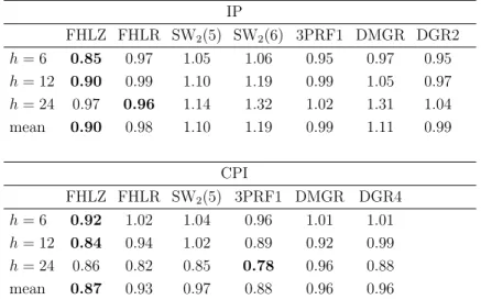
In Table 1 we report the average performance, measured by the RMSFE, of the three factor models (and the Alternative Methods) relative to AR. We give results for the Great Moderation, or pre-crisis period, starting with February 1985 and ending at December 2007, the beginning of the Great Recession (from December 2007 to June 2009), Panel A, and the full sample period, from February 1985 to September 2014, Panel B.
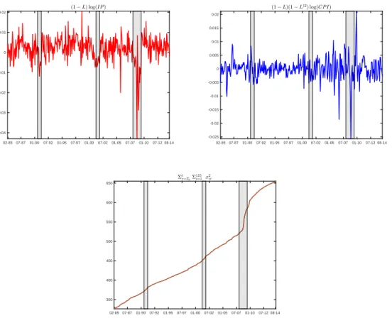
There are two strong reasons for splitting the sample. Firstly, IP, CPI and the whole dataset exhibit marked instability during the Great Recession. Regarding IP and CPI, this is clearly visible in the plot of the targets (1−L) log(IP) and
(1−L)(1−L12) log(CPI), see Figure 1, top graphs. We observe a marked change
in the mean of the first in the Great Recession. The second is stable in the mean, though exhibiting two outliers. Regarding the whole dataset, a marked change in its covariance structure is roughly but convincingly illustrated in the lower graph of Figure 1, where we plot the sum of squares Pt
τ=T0
P115
i=1x 2
iτ, for t running from
February 1985 to August 2014, the sample proper (recall thatxiτ is the dataset after
transformation and normalization, see Section 3.1). We observe a steady growth with a particularly sharp increase in the slope during the Great Recession.
Secondly, as a consequence of that instability, the relative forecasting performance of the factor models and the AR changes dramatically during the Great Recession. This is clearly illustrated in Figures 2 and 3. The solid line is the graph of the difference between the Square Forecast Error with methods m1 and m2, FHLZ and
SW for example, relative to IP and CPI, at each horizon, normalized by its estimated
standard deviation and smoothed by a centered moving average of length M =
61, with the coefficients equal to 1/M. Giacomini and Rossi (2010) use it to test against the null of equal local performance of two forecasting methods. The zero horizontal line indicates equal performance, the dotted lines indicate the 5-percent critical values, so thatm1 outperforms (underperforms) m2 locally, at the 5-percent
significance level, when the solid line is below (above) the lower (upper) dashed line. Because the moving averages are of length 61 and centered, the first and last 30 values are not computed or graphed.
In addition to testing for local equal performance, limiting the sample to the relatively stable pre-crisis period, we use the Diebold-Mariano test (see Diebold and Mariano (1995)) against the null of global equal performance of two predictors. Our main results are:
IP. FHLZ outperforms the other three methods in the pre-crisis period on average over the three horizons. It is slightly outperformed by FHLR at horizon 24, see Panel A in Table 1. The null of equal performance with FHLZ, in the pre-crisis period, is rejected for AR (at the 1% significance level), SW (at 5% for horizon 6 and 12, 10% for horizon 24). It is also rejected at the 10% level
for FHLR for horizons 6 and 12. All thep-values are reported in Table 2. The performance of FHLZ is somewhat improving before the crisis with respect to the three other methods at horizons 12 and 24, see Figure 2. During the crisis, see again Figure 2, SW and FHLR behave significantly (Giacomini-Rossi test) better than FHLZ and AR, while AR performs significantly better than FHLZ. However, with the end of the crisis almost all the solid lines are clearly heading back to the pre-crisis pattern. On average over the whole sample, FHLZ is outperformed by FHLR and SW at horizons 6 and 12. All methods do better than AR with the exception of SW at horizon 24, see Panel B in Table 1. CPI. FHLZ outperforms the other three methods in the pre-crisis period on average
over the three horizons. It is however outperformed at horizon 24 by FHLR and, slightly, SW, see Panel A in Table 1. The null of equal performance with FHLZ, in the pre-crisis period, is rejected for AR (at levels 10%, 5% and 1%), SW (at 10% for horizon 6 and 12). It is also rejected at the 10% level for FHLR for horizon 6, see Table 2. In this case the crisis has a negative effect on the performance of all three factor methods as compared to AR, see Figure 3. However, on average over the full sample, the best method remains FHLZ, with the exception of horizon 24, for which it is outperformed by SW. In many cases, though not as regularly as for IP, with the end of the crisis the solid lines in Figure 3 go back to the pre-crisis pattern.
To understand our results let us recall that the factor models employed here are based on the assumption of stationarity and co-stationarity (after suitable transfor-mations) of the variables in the dataset, while the AR method only requires sta-tionarity of the variable to be predicted. During the Great Moderation, when such assumptions are by and large fulfilled, the relative performance of the factor models and the AR change little, see again the pre-crisis period in Figures 2 and 3. In par-ticular, FHLZ outperforms the other methods, consistently with the results obtained with simulated stationary data in Forni et al. (2017). On the other hand, as soon as the crisis breaks out, as already observed,
behavior, see again Figure 1, top graphs. Both the factor and the AR models are affected.
(II) The autocovariance structure of the dataset changes abruptly, see again Figure 1, lower graph. This instability, affecting only the factor models, causes a deterioration in the estimation of the factors and of the loadings, i.e. the coefficients in (2.4), (2.10), (2.12).
In the case of CPI, where instability (I) is mild, all factor models loose ground with respect to the AR model. FHLZ remains the best method in the full sample, though by little with respect to AR. Moreover, the performance of the factor models relative to one another does not change much.
In the case of IP, where the instability (I) is much more important. The AR model, which is only based on the target, is strongly affected and its performance looses ground with respect to FHLR and SW. On the other hand, FHLZ, which is more dependent on the stationarity assumptions than the other factor models, looses ground with respect to all other methods.
The results for 3PRF, DGR and DMGR, see Sections 2.4 and 3.2.3, are reported in Table 1, last three columns.
IP. In the pre-crisis period 3PRF and DGR are very close on average to FHLR and therefore outperform SW but are outperformed by FHLZ. DMGR is outper-formed by AR. In the crisis period all the Alternative Methods perform poorly, so that none of them outperforms on average AR in the full sample.
CPI. In the pre-crisis period 3PRF performs on average like FHLZ, this being the result of a very good performance at horizon 24. DMGR and DGR perform like SW. In the full-sample period DMGR performs extremely well at horizon 24 and, in spite of the bad performance at horizon 6, slightly outperforms FHLZ on average.3
3Our result with DMGR on CPI, a good performance during the crisis as opposed to the
great-moderation period, is consistent with Table 2, p. 323 in De Mol et al. (2008), where the performance is very good for the period 1971-1984 but poor for 1985-2002.
Summing up, FHLZ is confirmed as the best method in the pre-crisis period both for IP and CPI, FHLR as the best for IP in the full sample, while DMGR has the best performance for CPI in the full sample.
4.2
Forecasting the whole dataset
We now extend the pseudo real-time comparison of our four methods to the whole dataset. For some of the variables the AR method outperforms the factor models. Precisely, we find that for 23 variables the AR outperforms by at least 10 percent all the factor models for at least one prediction horizon. This subset of variables, which includes housing, category 4 in Table ??, Appendix ??, is excluded.4
For real variables we use the specifications adopted for IP (we only ran SW2(5)),
while for the nominal variables those adopted for CPI. For every group of variables, in Table 3 we report the mean RMSE within the group. The best performance is given in bold. We see that FHLZ and FHLR generally perform better than SW, the latter being the most accurate only for employment 6 and 12 steps ahead. All in all, FHLR is more accurate for the real variables, i.e. IP, Employment, Unemployment Rate, Inventories, while FHLZ is more accurate for nominal variables, i.e. Prices, Wages, Interest Rates, Money and Stock Prices. For Exchange Rates and Wages at horizon 12 the AR is still the most accurate model. Considering median values rather than means we obtain similar results.
In Table 4 the distribution of the RMSE of the models is calculated excluding the same variables as before. Only FHLZ improves at every horizon upon AR for more than the half of the series. FHLR does so only 24-step ahead, is less accurate than AR 6-step ahead by 4.1 percent and 2.1 percent 12-step ahead. Furthermore, FHLZ is roughly as accurate as AR even at his 75-th percentile. SW is outperformed
by frequency domain models at most percentiles and horizons. Its performance
deteriorates as the predictive horizon increases while the contrary holds for FHLR and FHLZ. Among the frequency domain methods FHLZ performs better at the
4This result holds for our monthly dataset. In other works, with quarterly datasets, dynamic
factor models are successfully applied to housing market data, see Luciani (2015), Stock and Watson (2008) and Moench and Ng (2011).
95-th percentile and FHLR is more accurate at the 5-th percentile.
5
Conclusions
The paper has compared the forecasting performance of FHLZ, FHLR, SW and AR for a U.S. dataset including the Great Moderation, the Great Recession and the subsequent recovery.
We find that during the Great Moderation, when the dataset is relatively stable, FHLZ significantly prevails for both IP and CPI.
Over the full sample, the performance of FHLZ remains the best for CPI, though all factor models loose ground with respect to the simple AR model. FHLR and SW, in this order, become the best models for IP, thus exhibiting more robustness than FHLZ in a situation where both the target variable and the whole dataset undergo instability.
Forecasting each single series in the U.S. dataset for the full sample confirms the above results, with FHLZ being the best method for the nominal variables, FHLR for the real variables.
A robustness check of the results obtained with the U.S. data has been conducted on a European dataset consisting of 176 macroeconomic and financial time series for the Euro Area, observed at monthly frequency between January 1985 and August
2016, see Appendix ?? for details. The performance of the three factor models,
relative to one another, is confirmed in the pre-crisis period. In the full sample FHLR is the best method, albeit slightly, for both IP (as with the U.S. dataset) and CPI. However, with respect to the U.S. dataset, an important difference is the bad performance of all the factor models relative to AR for CPI in the pre-crisis period. See the results in Appendix ??.
Based on the data, U.S. and European, and the models employed in the present paper: (a) In stable periods FHLZ can be strongly recommended for IP and CPI; (b) when the data include unstable subperiods, such as the Great Recession, FHLR can be recommended for IP, FHLZ and FHLR for CPI.
and factor-based forecasts has been studied and discussed in Stock and Watson (2002a), D’Agostino et al. (2007), Banerjee et al. (2008), Stock and Watson (2009), D’Agostino et al. (2013), Clements (2015). The present paper however is the first to consider the effect of the Great Recession and the subsequent recovery in a pseudo real-time forecasting exercise using factor models.5
5More recent research has focused on (i) detecting different forms of instability in factor models,
see e.g. Breitung and Eickmeier (2011), Han and Inoue (2014), Yamamoto and Tanaka (2015), Chen et al. (2014), Barigozzi et al. (2016), (ii) consistent factor estimation under breaks, Bates et al. (2013), Ma and Su (2016), Cheng et al. (2016), Massacci (2016), (iii) modeling time varying factor models Del Negro and Otrok (2008), Mikkelsen et al. (2015). However, in our knowledge, no attempt has been made so far to use these models in a pseudo real-time forecasting exercise.
References
Albano, D. (2016). Latent factors in large-dimensional datasets: forecasting and data analysis using factor models. PhD thesis, Universit`a degli Studi di Napoli Federico II.
Alessi, L., Barigozzi, M., and Capasso, M. (2010). Improved penalization for deter-mining the number of factors in approximate factor models.Statistics & Probability Letters, 80(23–24):1806–1813.
Amengual, D. and Watson, M. W. (2007). Consistent estimation of the number of dynamic factors in a large N and T panel. Journal of Business & Economic Statistics, 25(1):91–96.
Anderson, B. and Deistler, M. (2008). Properties of zero-free transfer function matri-ces. SICE Journal of Control, Measurement and System Integration, 1(4):284–92. Bai, J. and Ng, S. (2002). Determining the number of factors in approximate factor
models. Econometrica, 70(1):191–221.
Banerjee, A., Marcellino, M., and Masten, I. (2008). Forecasting macroeconomic variables using Diffusion Indexes in short samples with structural change. In Fore-casting in the presence of structural breaks and model uncertainty, volume 3 of Frontiers of Economics and Globalization, pages 149–194. Emerald Group Pub-lishing.
Barigozzi, M., Cho, H., and Fryzlewicz, P. (2016). Simultaneous multiple change-point and factor analysis for high-dimensional time series. arXiv:1612.06928 [stat]. Bates, B. J., Plagborg-M¨oller, M., Stock, J. H., and Watson, M. W. (2013). Consis-tent factor estimation in dynamic factor models with structural instability. Journal of Econometrics, 177(2):289–304.
Boivin, J. and Ng, S. (2005). Understanding and comparing factor-based forecasts. International Journal of Central Banking, 1(3).
Breitung, J. and Eickmeier, S. (2011). Testing for structural breaks in dynamic factor models. Journal of Econometrics, 163(1):71–84.
Chen, L., Dolado, J., and Gonzalo, J. (2014). Detecting big structural breaks in large factor models. Journal of Econometrics, 180(1):30–48.
Cheng, X., Liao, Z., and Schorfheide, F. (2016). Shrinkage estimation of
high-dimensional factor models with structural instabilities. The Review of Economic Studies, 83(4):1511–1543.
Clements, M. P. (2015). Real-time factor model forecasting and the effects of insta-bility. Computational Statistics & Data Analysis. to appear.
D’Agostino, A., Gambetti, L., and Giannone, D. (2013). Macroeconomic forecasting and structural change. Journal of Applied Econometrics, 28(1):82–101.
D’Agostino, A. and Giannone, D. (2012). Comparing alternative predictors based on large-panel factor models. Oxford Bulletin of Economics and Statistics, 74(2):306– 326.
D’Agostino, A., Giannone, D., and Surico, P. (2007). (Un)Predictability and macroe-conomic stability. CEPR Discussion Paper 6594, C.E.P.R. Discussion Papers. De Mol, C., Giannone, D., and Reichlin, L. (2008). Forecasting using a large number
of predictors: Is bayesian shrinkage a valid alternative to principal components? Journal of Econometrics, 146(2):318–328.
Del Negro, M. and Otrok, C. (2008). Dynamic factor models with time-varying parameters: measuring changes in international business cycles. SSRN Scholarly Paper ID 1136163, Social Science Research Network, Rochester, NY.
den Reijer, A. H. J. (2005). Forecasting Dutch GDP using large scale factor models. DNB Working Paper 2005/28, De Nederlandsche Bank.
Diebold, F. X. and Mariano, R. S. (1995). Comparing predictive accuracy. Journal of Business & Economic Statistics, 13(3):253–263.
Doz, C., Giannone, D., and Reichlin, L. (2011). A Quasi–Maximum Likelihood
approach for large, approximate Dynamic factor models. Review of Economics
and Statistics, 94(4):1014–1024.
Eickmeier, S. and Ziegler, C. (2008). How successful are dynamic factor models at forecasting output and inflation? A meta-analytic approach. Journal of Forecast-ing, 27(3):237–265.
Forni, M., Giannone, D., Lippi, M., and Reichlin, L. (2009). Opening the black
box: structural factor models with large cross sections. Econometric Theory,
25(05):1319–1347.
Forni, M., Hallin, M., Lippi, M., and Reichlin, L. (2000). The generalized dynamic-factor model: Identification and estimation. Review of Economics and Statistics, 82(4):540–554.
Forni, M., Hallin, M., Lippi, M., and Reichlin, L. (2005). The generalized dynamic
factor model: One-sided estimation and forecasting. Journal of the American
Statistical Association, 100:830–840.
Forni, M., Hallin, M., Lippi, M., and Zaffaroni, P. (2015). Dynamic factor model with infinite dimensional factor space: Representation. Journal of Econometrics, 185:359–371.
Forni, M., Hallin, M., Lippi, M., and Zaffaroni, P. (2017). Dynamic factor models with infinite-dimensional factor spaces: Asymptotic analysis. Journal of Econo-metrics, 199(1):72–92.
Giacomini, R. and Rossi, B. (2010). Forecast comparisons in unstable environments. Journal of Applied Econometrics, 25(4):595–620.
Hallin, M. and Liˇska, R. (2007). Determining the number of factors in the general dy-namic factor model.Journal of the American Statistical Association, 102(478):603– 617.
Han, X. and Inoue, A. (2014). Tests for parameter instability in dynamic factor
models. Econometric Theory, pages 1–36.
Kapetanios, G. and Marcellino, M. (2009). A parametric estimation method for
dynamic factor models of large dimensions. Journal of Time Series Analysis,
30:208–238.
Kelly, B. and Pruitt, S. (2015). The three-pass regression filter: A new approach to forecasting using many predictors. Journal of Econometrics, 186(2):294–316. Luciani, M. (2015). Monetary policy and the housing market: A structural factor
analysis. Journal of Applied Econometrics, 30(2):199–218.
Ma, S. and Su, L. (2016). Estimation of large dimensional factor models with an unknown number of breaks. Working Paper 05-2016, Singapore Management Uni-versity, School of Economics.
Massacci, D. (2016). Unstable diffusion indexes: With an application to Bond Risk Premia. SSRN Scholarly Paper ID 2816534, Social Science Research Network, Rochester, NY.
McCracken, M. W. and Ng, S. (2016). FRED-MD: A Monthly Database for macroe-conomic research. Journal of Business & Economic Statistics, 34(4):574–589. Mikkelsen, J. G., Hillebrand, E., and Urga, G. (2015). Maximum Likelihood
Estima-tion of time-varying loadings in high-dimensional factor models. CREATES Re-search Paper 2015-61, Department of Economics and Business Economics, Aarhus University.
Moench, E. and Ng, S. (2011). A hierarchical factor analysis of U.S. housing market
dynamics. The Econometrics Journal, 14(1):C1–C24.
Onatski, A. (2009). Testing hypotheses about the number of factors in large factor models. Econometrica, 77(5):1447–1479.
Pe˜na, D. and Poncela, P. (2004). Forecasting with nonstationary dynamic factor models. Journal of Econometrics, 119(2):291–321.
Schumacher, C. (2007). Forecasting German GDP using alternative factor models based on large datasets. Journal of Forecasting, 26(4):271–302.
Stock, J. and Watson, M. (2009). Forecasting in dynamic factor models subject to structural instability.The Methodology and Practice of Econometrics. A Festschrift in Honour of David F. Hendry, 173:1–57.
Stock, J. H. and Watson, M. W. (2002a). Forecasting using principal components from a large number of predictors. Journal of the American Statistical Association, 97(460):1167–1179.
Stock, J. H. and Watson, M. W. (2002b). Macroeconomic forecasting using diffusion indexes. Journal of Business & Economic Statistics, 20(2):147–162.
Stock, J. H. and Watson, M. W. (2005). Implications of dynamic factor models for VAR analysis. NBER Working Paper 11467, NBER.
Stock, J. H. and Watson, M. W. (2008). The evolution of national and regional factors in US housing construction. Princeton University.
Stock, J. H. and Watson, M. W. (2012). Generalized shrinkage methods for forecast-ing usforecast-ing many predictors. Journal of Business & Economic Statistics, 30(4):481– 493.
Timmermann, A. (2006).Forecast Combinations, volume 1 ofHandbook of Economic
Forecasting, chapter 4, pages 135–196. Elsevier.
Yamamoto, Y. and Tanaka, S. (2015). Testing for factor loading structural change
Table 1: Mean Square Forecast Error Relative to AR for U.S. data
PANEL A: Pre Crisis (1985 : 1 - 2007 : 11) IP FHLZ FHLR SW2(5) SW2(6) 3PRF1 DMGR DGR2 h= 6 0.85 0.97 1.05 1.06 0.95 0.97 0.95 h= 12 0.90 0.99 1.10 1.19 0.99 1.05 0.97 h= 24 0.97 0.96 1.14 1.32 1.02 1.31 1.04 mean 0.90 0.98 1.10 1.19 0.99 1.11 0.99 CPI FHLZ FHLR SW2(5) 3PRF1 DMGR DGR4 h= 6 0.92 1.02 1.04 0.96 1.01 1.01 h= 12 0.84 0.94 1.02 0.89 0.92 0.99 h= 24 0.86 0.82 0.85 0.78 0.96 0.88 mean 0.87 0.93 0.97 0.88 0.96 0.96
PANEL B: Full Sample (1985 : 1 - 2014 : 8) IP FHLZ FHLR SW2(5) SW2(6) 3PRF1 DMGR DGR2 h= 6 0.95 0.87 0.86 0.90 1.09 0.97 1.14 h= 12 0.94 0.88 0.86 0.98 0.99 1.09 1.11 h= 24 0.97 0.93 1.06 1.17 0.97 1.09 1.03 mean 0.95 0.89 0.93 1.02 1.02 1.05 1.09 CPI FHLZ FHLR SW2(5) 3PRF1 DMGR DGR4 h= 6 0.95 1.09 1.14 0.99 1.04 1.19 h= 12 0.98 1.15 1.06 1.00 0.98 1.17 h= 24 1.04 1.01 0.95 1.02 0.90 1.10 mean 0.99 1.08 1.05 1.00 0.97 1.15
Notes. Mean Square Forecast Error (MSFE), relative to AR, for IP and CPI, in the Pre-Crisis
and the Full-Sample periods. For IP we display both the results of SW2(6), the method selected
in the calibration sample, and SW2(5). The methods compared are the three factor models and
Table 2: Diebold-Mariano test for the pre-crisis period: p-values IP FHLZ vs SW2(5) FHLR vs SW2(5) FHLZ vs FHLR FHLZ vs AR FHLR vs AR SW2(5) vs AR SW2(6) vs AR h=6 0.05 0.03 0.10 0.00 0.44 0.68 0.72 h=12 0.05 0.03 0.11 0.00 0.48 0.78 0.94 h=24 0.07 0.04 0.56 0.09 0.25 0.91 0.98 CPI FHLZ vs SW FHLR vs SW FHLZ vs FHLR FHLZ vs AR FHLR vs AR SW vs AR h=6 0.07 0.22 0.08 0.09 0.53 0.58 h=12 0.07 0.02 0.15 0.02 0.31 0.53 h=24 0.52 0.32 0.60 0.01 0.17 0.26
Notes. Due to instability, the Diebold-Mariano p-values are not computed for the full
Table 3: Mean MSFE, relative to AR, by category FHLZ h= 6 h= 12 h= 24 IP∗ 0.95 0.92 0.98 Employment 1.13 1.07 0.98 Unemployment Rate 0.87 0.91 0.94 Inventories 1.00 0.93 0.98 Prices 0.98 1.01 0.99 Wages 0.98 0.99 0.99 Interest Rates 0.99 0.98 0.95 Money 0.87 0.86 0.75 Exchange Rates 1.01 1.01 1.01 Stock Prices 0.97 0.97 0.94 FHLR h= 6 h= 12 h= 24 IP∗ 0.93 0.90 0.97 Employment 0.98 0.95 0.91 Unemployment Rate 0.67 0.72 0.85 Inventories 0.95 0.89 0.97 Prices 1.11 1.15 1.03 Wages 1.08 1.05 0.97 Interest Rates 1.12 1.14 1.07 Money 0.90 0.93 0.79 Exchange Rates 1.07 1.07 1.01 Stock Prices 1.02 1.09 1.01 SW h= 6 h= 12 h= 24 IP∗ 0.95 0.91 1.11 Employment 0.94 0.94 1.00 Unemployment Rate 0.68 0.74 0.97 Inventories 1.04 0.97 1.24 Prices 1.22 1.16 1.07 Wages 1.15 1.12 1.12 Interest Rates 1.32 1.52 1.55 Money 0.98 0.94 0.88 Exchange Rates 1.18 1.15 1.14 Stock Prices 1.25 1.34 1.30
Notes. MSFE, relative to AR, in the full sample, averaged over the variables belonging to each
category (23 variables are excluded, see Section 4.2). The three factor models are compared. For SW the specification is SW2(5). The best result for each horizon, over the three methods, in bold.
Table 4: Distribution MSFE relative to AR FHLZ Percentile: 0.05 0.25 0.50 0.75 0.95 h= 6 0.82 0.92 0.99 1.02 1.22 h= 12 0.84 0.92 0.98 1.01 1.14 h= 24 0.82 0.94 0.98 1.01 1.07 FHLR Percentile: 0.05 0.25 0.50 0.75 0.95 h= 6 0.64 0.93 1.04 1.12 1.18 h= 12 0.67 0.91 1.02 1.14 1.26 h= 24 0.77 0.90 0.98 1.06 1.21 SW Percentile: 0.05 0.25 0.50 0.75 0.95 h= 6 0.65 0.95 1.12 1.23 1.38 h= 12 0.67 0.91 1.07 1.19 1.61 h= 24 0.73 0.96 1.07 1.29 1.63
Notes. Distribution of MSFE, relative to AR, in the full sample, over 92 variables belonging to
Figure 1: Instability of IP, CPI and the whole dataset in the Great Recession 02-8507-87 01-90 07-92 01-95 07-97 01-00 07-02 01-05 07-07 01-10 07-12 08-14 -0.04 -0.03 -0.02 -0.01 0 0.01 0.02 02-8507-87 01-90 07-92 01-95 07-97 01-00 07-02 01-05 07-07 01-10 07-12 08-14 -0.025 -0.02 -0.015 -0.01 -0.005 0 0.005 0.01 0.015 0.02 02-85 07-8701-90 07-92 01-95 07-97 01-00 07-02 01-05 07-07 01-10 07-12 08-14 350 400 450 500 550 600 650
Notes. In the top graphs the variables x1t = (1−L) log IPt and x77,t = (1 −L)(1−
L12) log CPIt (recession periods in grey). Both show a marked departure from the
station-arity assumption during the Great Recession. Rough evidence of the instability of the whole dataset is given in the lower graph, showing the cumulated sum of P
ix2iτ,i= 1, . . . ,115,
Figure 2: Fluctuation test (IP) FHLZ vs FHLR 1985 1990 1995 2000 2005 2010 2015 -4 -2 0 2 4 6 8 10 1985 1990 1995 2000 2005 2010 2015 -4 -2 0 2 4 6 8 10 1985 1990 1995 2000 2005 2010 2015 -5 0 5 10 15 FHLZ vs SW 1985 1990 1995 2000 2005 2010 2015 -4 -2 0 2 4 6 8 10 1985 1990 1995 2000 2005 2010 2015 -4 -2 0 2 4 6 8 10 1985 1990 1995 2000 2005 2010 2015 -10 -5 0 5 10 FHLZ vs AR 1985 1990 1995 2000 2005 2010 2015 -15 -10 -5 0 5 10 15 1985 1990 1995 2000 2005 2010 2015 -25 -20 -15 -10 -5 0 5 1985 1990 1995 2000 2005 2010 2015 -10 -5 0 5 10 15 FHLR vs SW 1985 1990 1995 2000 2005 2010 2015 -10 -5 0 5 10 15 1985 1990 1995 2000 2005 2010 2015 -4 -2 0 2 4 6 8 10 1985 1990 1995 2000 2005 2010 2015 -15 -10 -5 0 5 FHLR vs AR 1985 1990 1995 2000 2005 2010 2015 -15 -10 -5 0 5 1985 1990 1995 2000 2005 2010 2015 -15 -10 -5 0 5 1985 1990 1995 2000 2005 2010 2015 -15 -10 -5 0 5 SW vs AR 1985 1990 1995 2000 2005 2010 2015 -10 -8 -6 -4 -2 0 2 4 1985 1990 1995 2000 2005 2010 2015 -10 -8 -6 -4 -2 0 2 4 1985 1990 1995 2000 2005 2010 2015 -10 -5 0 5 10
Notes. Fluctuation test statistic: Solid. 5 % critical value: Dotted. If the solid is below the
Figure 3: Fluctuation test (CPI) FHLZ vs FHLR 1985 1990 1995 2000 2005 2010 2015 -15 -10 -5 0 5 1985 1990 1995 2000 2005 2010 2015 -15 -10 -5 0 5 1985 1990 1995 2000 2005 2010 2015 -15 -10 -5 0 5 10 15 FHLZ vs SW 1985 1990 1995 2000 2005 2010 2015 -15 -10 -5 0 5 1985 1990 1995 2000 2005 2010 2015 -10 -5 0 5 10 1985 1990 1995 2000 2005 2010 2015 -4 -2 0 2 4 6 8 10 FHLZ vs AR 1985 1990 1995 2000 2005 2010 2015 -10 -5 0 5 10 15 20 1985 1990 1995 2000 2005 2010 2015 -5 0 5 10 15 1985 1990 1995 2000 2005 2010 2015 -10 -5 0 5 10 15 FHLR vs SW 1985 1990 1995 2000 2005 2010 2015 -20 -15 -10 -5 0 5 10 1985 1990 1995 2000 2005 2010 2015 -4 -2 0 2 4 6 8 10 1985 1990 1995 2000 2005 2010 2015 -5 0 5 10 15 FHLR vs AR 1985 1990 1995 2000 2005 2010 2015 -5 0 5 10 15 20 1985 1990 1995 2000 2005 2010 2015 -5 0 5 10 15 1985 1990 1995 2000 2005 2010 2015 -10 -5 0 5 10 15 SW vs AR 1985 1990 1995 2000 2005 2010 2015 -5 0 5 10 15 1985 1990 1995 2000 2005 2010 2015 -5 0 5 10 15 20 1985 1990 1995 2000 2005 2010 2015 -10 -5 0 5 10
Notes. Fluctuation test statistic: Solid. 5 % critical value: Dotted. If the solid is below the