Conditional-Functional-Dependencies Discovery
Raoul Medina1 Lhouari Nourine2
Research Report LIMOS/RR-08-13 19 d´ecembre 2008
2[email protected], Universit´e Blaise Pascal – LIMOS – Campus des C´ezeaux – 63173 Aubi`ere Cedex, France
Abstract
Conditional Functional Dependencies (CFDs) are Functional Dependencies (FDs) that hold on a fragment relation of the original relation. In this paper, we show the hierarchy between FDs, CFDs and Association Rules (ARs): FDs are the union of CFDs while CFDs are the union of ARs. We propose a general method to discover a minimal non redundant cover of a relation consisting of FDs, pure CFDs and pure ARs. We also show the link between Approximate Functional Dependencies (AFDs) and approximate ARs. Consequence of our study is that any algorithm which computes ARs could be used to find FDs and CFDs too. We also establish the link between the problem of finding equivalent pattern tableaux of a CFD and the problem of finding keys of a relation.
1
Introduction
Dependency theory is one of the major part of database theory and has been traditionally used to optimize queries, prevent invalid updates and to nor-malize databases. Originally, dependency theory has been developed for un-interpreted data and served mainly database conception purposes [10]. The Functional Dependencies introduced by Codd were generalized to Equality Generating Dependencies (EGD) [4]. In [3], dependencies over interpreted data (i.e. equality requirements are replaced by constraints of an inter-preted domain) were introduced and generalized the EGDs into Constraint-Generating-Dependencies (CGD). In [7], authors present a particular case of CGDs: Conditional Functional Dependencies (CFDs), for data cleaning purposes. CFDs are dependencies which holds on instances of the relations. Constraint used in CFDs is the equality and allows to fix particular constant values for attributes. Basically, CFDs can be viewed as FDs which holds on a fragment relation of the original instance relation, this fragment relation being characterized by the constraints to apply on the attributes. Those constraints represent a selection operation on the relation. All these works focused mainly on implication analysis and axiomatizability.
Discovery of dependencies existing in an instance of a relation received considerable interest as it allowed automatic database analysis. Knowledge discovery and data mining [1], database management ([5],[9]), reverse engi-neering [17] and query optimization [18] are among the main applications benefiting from efficient dependencies discovery algorithms. New dependen-cies on instances of relations where defined. We cite (among others): Asso-ciation Rules (AR) [1] which are dependencies holding on particular values of attributes, and Approximate Functional Dependencies (AFD) [13] which are FDs which almost hold on a given relation. Note that AFDs have also applications in database design [11]. For those latter dependencies, several measures of approximateness were defined, expressing the interest of the de-pendency. Numerous algorithms have been proposed for such dependencies discovery, usually ad-hoc algorithms discovering a particular type of depen-dency. Among the most famous algorithms we can cite: A PRIORI [1] (a level-wise frequent itemsets discovery approach) for ARs mining, TANE [13] (similar approach as A PRIORI but for FDs and AFDs discovery), Close [15] (discovery of closed frequent itemsets). Usually, algorithms used to discover FDs can be adapted to discover ARs and reciprocally. For the moment, no algorithm has been proposed to discover CFDs or CGDs in a relation.
Contributions: In this paper, we study the link between ARs, CFDs and FDs. We show that CFDs are the union of ARs and FDs are the union of CFDs (section 2). Based on this hierarchy among ARs, CFDs and FDs, we propose a general approach for discovering a minimal non redundant cover containing FDs, CFDs which do not generalize in FDs and ARs which cannot be generalized in CFDs. We also study how a CFD can be expressed
equivalently using different constraints. We show that finding all minimal constraints to express the same CFD is equivalent to the problem of finding minimal keys of a relation (section 3). We also show the link between AFDs and approximate ARs (association rules that almost hold in a relation): an AFD can be seen as the union of ARs and approximate ARs. We show that any algorithm that computes ARs can thus be used to compute CFDs, AFDs and FDs (section 4). We also discuss our results and relate them with existing results (section 5).
2
Background, Definitions and Preliminary
Re-sults
2.1 Definitions
Let R be a relation schema defined over a set of attributes Attr(R). The domain of each attribute A ∈ Attr(R) is denoted by Dom(A). For an instance r of R, a tuple t∈ r and X a sequence of attributes, we use t[X] to denote the projection oftonto X.
An FD X → Y, where X, Y ⊆ Attr(r), is satisfied by r, denoted by
rX→Y, if for all pairs of tuplest1, t2 ∈r we have: ift1[X] =t2[X] then t1[Y] = t2[Y]. In other words, all pairs of tuples agreeing on attributes X will agree on attributes Y.
A CFD ϕ defined on R is a pair (X → Y, Tp), where (1) X → Y is a
standard FD, referred to as the FD embedded inϕ; and (2)Tp is a tableau
with attributes inR, referred to as the pattern tableau ofϕ, where for each
A∈Attr(R) and each pattern tupletp ∈Tp,tp[A] is either:
• a constant ’a’ inDom(A),
• an unamed variable⊤that draws values from Dom(A),
• or an empty variable ⊥which indicates that the attribute does not contribute to the pattern (i.e. A6∈X∪Y). 3
For any constantaof an attribute we have: ⊥ ≤a≤ ⊤. We define the pattern intersection operator ⊓of two tuples as:
t1⊓t2=tp such that∀A∈Attr(r),
tp[A] =t1[A], Eifˆ t1[A]≤t2[A] tp[A] =t2[A], Eifˆ t1[A]> t2[A] tp[A] =⊥, otherwise.
We define the pattern restriction to attributes X of a tuple t, denoted by
3
t(X) as:
t(X) =tp such that∀A∈Attr(r),
(
tp[A] =t[A], Eifˆ A∈X
tp[A] =⊥, otherwise.
We define a subsumption operator ⊑over pattern tuplest1 and t2:
t1⊑t2 if and only if ∀A∈Attr(R), t1[A]≤t2[A].
In other words, t1 ⊑ t2 if and only if t1 ⊓t2 = t1. We define the special tuple T opas the tuple with value ⊤on all attributes, i.e. tp ⊑T op for any
pattern tupletp.
An instance r of R satisfies the CFD ϕ, denoted by r ϕ, if for each
tuple tp in the pattern tableau Tp of ϕ, and for each pair of tuples t1, t2 in
r, if t1(X) =t2(X)⊑tp(X), then t1(Y) =t2(Y)⊑tp(Y).
A pattern tuple tp defines a fragment relation of r:
rtp={t∈r|tp ⊑t}.
We will denote byrTp the fragment relation containing all tuples of r satis-fying at least one of the patterns inTp. Note that given a CFD (X →Y, Tp),
we thus haverTp X→ Y and r−rTp 6X →Y. For this reason, we will denote: rX→Y = rTp and rX6→Y = r−rTp. For convenience reason, for a CFDϕ= (X →A, TP), we will sometimes denote byrϕthe relation defined
byrTp, i.e. rϕ =rTp =rX→A.
As in [12], to simplify the discussion without losing generality, we con-sider CFDs of the form (X→A, Tp) where Ais a single attribute.
2.2 X-complete Relations
Definition 1 (X-complete property [11]) The relation r is said to be X-complete if and only if ∀t1, t2 ∈r we have t1[X] =t2[X].
In other words, a relation is X-complete if all tuples agree on the at-tributesX. Note that they might also agree on other attributes: this con-stitutes the pattern ofr.
Definition 2 (X-complete-pattern) We call X-complete-pattern of an
X-complete relationr, denoted byγ(X, r), the pattern tuple on which tuples of r agree. More formally: γ(X, r) =⊓ {t∈r}.
Note that since r is X-complete, its X-complete-pattern defines at least attributes in X (i.e. those attributes do not have the ⊥value). Given a relation r and a set of attributes it is always possible to horizontally decomposer in fragment relations which are X-complete.
Definition 3 (X-complete horizontal decomposition) We denote byRX(r)
the set of all X-complete fragment relations of r. More formally: RX(r) =
{r′⊆r|r′ is X-complete}.
In each fragment relations, tuples agree at least on the attributesX. Definition 4 (Set of X-patterns) We denote byΓ(X, r) the set of all X-complete-patterns of an X-complete decomposition. More formally: Γ(X, r) =
{γ(X, r′)|r′ ∈RX(r)}.
Attributes X are defined in all X-complete-patterns. Some others at-tributes might also be defined.
Definition 5 (Closure operator) We call closure of X in r, denoted by
θ(X, r), the set of all attributes defined in all X-complete-patterns of the relation. More formally:
θ(X, r) ={A∈Attr(r)| ∀tp ∈Γ(X, r), tp[A]6=⊥ }.
Using the closure operator θ(X, r), we can trivially characterize FDs. Property 1 Let A6∈X. We have r X →A (i.e. X →A is an FD of r)
if and only if A∈θ(X, r).
Note that the closure operator θ(X, r) is equivalent to the closure of a set of attributesX using FD ofr.
Proposition 1 Let r′ ⊆ r. Then r′ is X-complete if and only if r′ is
θ(X, r)-complete.
A consequence is that X and θ(X, r) define the sameX-complete hori-zontal decomposition ofr. Which leads to the following corollary.
Corollary 1 Γ(X, r) = Γ(θ(X, r), r).
2.3 Link Between CFDs, FDs and ARs
Here we show the relation between CFDs and other usual dependencies. FDs: An FD X → A can be seen as a CFD (X → A, tp) where tp is
a single tuple with no constants, i.e. tp = T op(X∪ {A}). In other words,
rX→A if and only ifrX→A=r (and thusrX6→A=∅).
ARs: An AR is a dependency (X1 =b1− ∧ · · · ∧(Xk=bk)→(A=a)
meaning that for any tuplet∈r, ift[X1] =b1 and · · · and t[Xk] =bk then
t[A] =a. Note that for this kind of dependency, contrary to FDs and CFDs, no agreement is needed among tuples. Thesupportof an AR is the number of tuples of the relation satisfying the dependency.
Lemma 1 Let r be a relation, X ⊆ Attr(r), such that r is X-complete. Then the following assertions are equivalent:
1. (X→A, γ(X, r)) is a CFD of r
2. X→A is an FD of r
3. X→A is an AR of r
Lemma 1 states that when a relation is X-complete, FDs, CFDs and ARs of the formX→Aare equivalent. Next theorem characterizes the link between FDs, CFDs and ARs when the relation is notX-complete.
Theorem 1 Let r a relation,X ⊆Attr(r),A∈Attr(r)\X andTp ={tp ∈
Γ(X, r)|tp[A]6=⊥ }. The following assertions are equivalent:
1. (X→A, Tp) is a CFD ofr
2. X→A is an FD of rTp
3. For any r′ ∈RX(rTp), X→A is an AR of r
′
Theorem 1 is quite important for understanding the link between ARs, CFDs and FDs. Indeed, it leads to a hierarchy among those dependencies:
• an AR X → A is a dependency that holds on at least one fragment relation ofr which isX-complete.
• a CFD (X → A, Tp) is a dependency that holds on some fragment
relations of r which are X-complete. It can thus be viewed as the union of ARs holding on those fragment relations.
• an FD is a dependency that holds on all fragment relations ofrwhich isX-complete. It can thus be viewed as the union of ARs holding on all those fragment relations.
We will say thatX→Ais a pure ARif it holds exactly on oneX-complete fragment relation. We will say that a CFD is a pure CFD if it holds on at least two X-complete fragment relations and does not hold on at least one X-complete fragment relations. In other words, a pure AR does not generalize in a CFD, while a pure CFD does not generalize in an FD. 2.4 Main Results
Definition 6 (A-Valid and A-Invalid X-complete pattern tuples) An
X-complete pattern tupletp is saidA-valid towardsAif and only if attribute
A is defined in tp.
We denote by Ψ(X → A) the set of all A-valid X-complete pattern tuples. More formally: Ψ(X→A) ={tp ∈Γ(X, r)|tp[A]6=⊥ }.
Dually, we denote byΨ(X6→A) the set of all A-invalidX-complete pattern tuples: Ψ(X 6→A) = Γ(X, r)−Ψ(X →A).
Theorem 2 Givenr a relation,X ⊆Attr(r) and an attribute A6∈X. The dependency X → A is a functional dependency of r (i.e. A ∈ θ(X, r)) if and only if Ψ(X6→A) =∅.
Theorem 2 could be rephrased by saying that X → A is an FD if and only if the dependency holds in all X-complete fragment relations. If the dependency does not hold in (at least) one of the X-complete fragment relations we thus have a CFD.
Corollary 2 Givenr a relation,X ⊆Attr(r)and an attributeA6∈X. The pair (X →A,Ψ(X →A)) is a CFD of r if and only if Ψ(X →A)6=∅ and Ψ(X6→A)6=∅.
3
Algorithms for CFD Discovery
From Theorem 2 and its Corollary 2 we can thus deduce an Apriori like na¨ıve algorithm: we search CFDs in the powerset ofAttr(r).
Algorithm 1: Na¨ıve Apriori-like algorithm Data: r a relation
Result: Σ the set of all CFDs begin Σ←− ∅ forall X ⊂Attr(r) do forall A6∈X do if Ψ(X6→A) =∅then Σ←−Σ∪ {(X →A, T op(X∪ {A})} else if Ψ(X→A)6=∅then Σ←−Σ∪ {(X →A,Ψ(X →A))} end
In the remaining of the paper, we show how a Close-like algorithm could be used: we search the closed sets lattice rather than the powerset.
3.1 A Close-like Approach
Main idea of this algorithm is to generate a subset of FDs and CFDs such that the others FDs and CFDs can be derived from this subset. We propose to generate FDs such that their left-part is a minimal generator and CFDs (or ARs) which are pure CFDs (pure ARs).
Definition 7 (Minimal generator) A subsetX of attributes of r is said to be a minimal generator of Γ(X, r) if and only if for any Y ⊂X we have
Γ(Y, r)6= Γ(X, r). By extension, we also say thatX is a minimal generator of θ(X, r).
Several algorithms proposed methods for computing minimal generators and their associated closed set: Close [15], Closet [16], Pascal [2], Charm [19]ˆE to name a few. Any of those algorithms could thus be adapted with our closure operator (based on pattern discovery).
Concerning the CFDs, we do not need to compute their minimal genera-tors. Indeed, we can keep one representative CFD for eachpureCFD. Next theorem characterizes this representative CFD.
Theorem 3 Let r be a relation, X ⊆ Attr(r) and A 6∈ X. We have:
r(X →A,Ψ(X→A)) if and only if r (θ(X, r)→A,Ψ(X →A)).
Generating CFDs of the form (θ(X, r) → A,Ψ(X → A)) is thus suffi-cient. Indeed, all other CFDs can be found as (Y →A,Ψ(X→A)) whereY
is a generator ofθ(X, r). Moreover, ifY 6=θ(X, r) thenθ(Y, r)→θ(X, r)−Y
is an FD. Main idea of our Close-like algorithm is thus to generate FDs such that their part is a minimal generator and CFDs such that their left-part is a closed set. With these informations, generating remaining FDs and CFDs is straightforward. Note that any algorithm which computes minimal generators and their associated closed sets could be adapted in order to gen-erate FDs and CFDs. For this reason, we do not detail the computation of minimal generators. For the same reason, we do not detail the computation of the patterns: it could be done either by parsing the relation for a whole set of generators (like in Close) or by computing intersection of list of tuples (in a similar way as TANE).
Theorem 4 Algorithm 2 computes all CFDs of the form (X →A, Tp)such
that:
• if Tp = {T op(X ∪ {A})} (i.e. it is an FD) then X is a minimal
generator of θ(X, r);
• otherwise X =θ(X, r).
Computing the patterns and the closures associated to each generators could be optimized, using the following proposition.
Proposition 2 Ψ(X →A)⊆Γ(X∪ {A}, r).
A consequence of Proposition 2 is that all X-complete fragment relations defined by pattern tuples in Ψ(X →A) are also X∪ {A}-complete. Those fragment relations will thus appear in theX∪ {A}-complete horizontal de-composition ofr. A consequence is that we do not need to re-compute their patterns. The remaining fragment relations appearing in the decomposition
Algorithm 2: Na¨ıve Close-like algorithm Data: r a relation
Result: Σ the set of minimal generators FD and closed CFD begin Σ←− ∅ Gen={{}} while Gen6=∅ do forall X ∈Gen do forall A6∈X do if A∈θ(X, r) then Σ←−Σ∪ {(X→A, T op(X∪ {A}))} else if Ψ(X →A)6=∅ then Σ←−Σ∪ {(θ(X, r)→A,Ψ(X →A))}
Gen←− Compute next minimal generators end
will simply correspond to the X∪ {A}-complete horizontal decomposition of the fragment relations defined by Ψ(X 6→ A). Thus, only their cor-responding patterns should be computed at the next step. Note that if Ψ(X 6→ A) = ∅ then RX(r) = RX∪{A}(r). Which leads to the following
corollary.
Corollary 3 Ψ(X 6→A) =∅ if and only if Γ(X, r) = Ψ(X→A) = Γ(X∪ {A}, r).
In other words, there are no A-invalid X-complete pattern tuples if and onlyA belongs toθ(X, r) (i.e. X is a generator ofθ(X, r)). Consequence of this corollary is that the patterns for X∪ {A} are exactly the same as the ones forX. Thus they already have been generated.
3.2 Constraint Satisfaction for Pattern Tableau Generation Given a CFD (X →A,Ψ(X →A)), the set Ψ(X →A) can be viewed as a selection query which returns the fragment relation satisfyingX→A. Any selection query returning a fragment relation satisfying X → A could thus be a valid pattern tableau for the CFD. In the same way, Ψ(X 6→A) is the query returning the fragment relation where X → A is not satisfied. We can thus view Ψ(X 6→A) as a set of constraints that should be satisfied in order notto have X→A:
C(X6→A) = _
t∈Ψ(X6→A)
^
B∈X
If we take the complementary constraint, we thus obtain the set of con-straints that should be satisfied in order to haveX→A satisfied.
C(X6→A) = ^
t∈Ψ(X6→A)
_
B∈X
B6=t[B]
Theorem 5 Given r a relation and (X →A,Ψ(X →A))a CFD of r then for any model m of C(X6→A), the pair(X→A, m) defines a CFD of r.
In other words, tableau of a CFD can be written in different ways. Any model of C(X 6→A) defines a selection query such that the resulting frag-ment relation satisfies X → A. Thus, the model could be used to define a pattern tuple of the tableau of the CFD (by setting to ⊤all attributes inX∪ {A} that do not appear in the model). Thus, finding tableaux of a CFD is equivalent to the problem of finding the models ofC(X6→A). The problem of finding the CFD of a relation can thus be expressed as finding the models of a particular constraint.
Problem 1 (All models) Input : C(X 6→A) Output : MALL={m|m is a model of C(X6→A)}.
Note that the fragment relation selected by the model might be empty. In this case the CFD trivially holds. However, in order to be meaningful, it would be preferable to find models which do return a non empty fragment relation.
Problem 2 (All models in r) Input : C(X 6→A), relation r
Output : MALL(r) ={m∈MALL| ∃t∈r, m ⊑t}.
To define a model of C(X 6→A) in the relation r, a pattern tuple tp has
to subsume at least one tuple of the relation and not subsume anyA-invalid pattern tuples in Ψ(X6→A). This condition can be simplified using pattern tuples in Ψ(X →A).
Proposition 3 Given a relation r, Ψ(X → A) and Ψ(X 6→ A), a pattern tuple m is a model of C(X 6→A) in r if and only if ∃tp ∈Ψ(X → A) and
∀t′
p∈Ψ(X6→A) we have t′p6⊑m andm ⊑tp.
Thus, any pattern tuple tp in Ψ(X → A) defines a sub-constraint of
C(X6→A), denoted byC(X 6→A)tp: only constant values intp are allowed
for the models. It is easy to check that any model of this sub-constraint is also a model of the global constraint. Such sub-constraint can be represented as a relation.
Definition 8 (Relations of models in r) Given tp ∈ Ψ(X → A), we
define the relation rtp(Ψ(X 6→ A)) = {tp(X) ⊓t
′
p(X) | t′p ∈ Ψ(X 6→
Any pattern m which subsumes tp(X) while not subsuming other
tu-ples in the relation rtp(Ψ(X 6→ A)) is thus a model. In other words, keys of rtp(Ψ(X 6→ A)) are models of C(X6→A). This is formalized by next theorem.
Theorem 6 The pattern tuple mp defines a model of C(X 6→A) in r if
and only if there exists tp ∈Ψ(X →A) such that γ(mp, rtp(Ψ(X 6→A))) =
tp(X).
Thus, to find models of C(X 6→A), one could use any algorithm which finds keys of a relation. Finding just minimal keys could be more interesting since all keys could be inferred from minimal keys.
Problem 3 (All minimal models in r) Input : C(X6→A), relation r
Output : MM IN ={m∈MALL(r)| ∀m′ ∈MALL(r), m′ 6⊆m}.
Finding all minimal models is equivalent to finding all minimal keys of the relations rtp(Ψ(X 6→ A)), for any tp ∈ Ψ(X → A). Note that such minimal models define minimal generators of the pattern tuples in Ψ(X→
A) and could thus be computed directly during the generation of the CFDs and FDs. If patterns associated to minimal generators of FDs are stored during the process, there is no need in computing the minimal models: we already have them in the patterns of the minimal generators. Otherwise, when patterns of minimal generators are not stored, computation of minimal models could be doneon demand.
4
Link Between CFDs, Approximate FDs and
Ap-proximate ARs
An AFD [13] is an FD that almost holds: some tuples of r invalidate the FD, representing errors or exceptions to the rule. Several ways of defining the approximateness of a dependency X → A have been used. The most common accepted measure is theg3 error, representing the fraction of rows that should be removed fromr in order to have r X→A. :
g3(X →A) = 1−
(max{|s| s.t. s⊆r∧sX →A})
|r|
We call support of an AFD X → A the size of the maximal fragment relationsmaxsuch thatsmaxX →A. Theg3error could thus be rewritten:
g3(X →A) = 1−
Support(X→A)
|r|
An approximate AR is, in the same way, an AR which almost holds on
(X →A, tp) is theconfidence conf((X →A, tp)), expressing the conditional
probability for a tuple t ∈ r of having t[X∪ {A}] = tp[X∪ {A}] knowing
thatt[X] =tp[X].
conf((X →A, tp)) =
|rtp(X∪{A})|
|rtp(X) |
Obviously, given a pure CFD (X →A, Tp),X →Ais an AFD. Moreover,
rX→A⊆smax. Thus we have|rTp |=|rX→A|≤Support(X →A). Missing tuples might be found inrX6→A.
For any pattern tuple tp in Ψ(X 6→ A), rtp 6 X → A by definition. However, if we consider RA(rtp), the A-complete horizontal decomposition of rtp, we have: ∀r ′ ∈R A(rtp), r ′ X → A. Thus,r Tp∪r ′ X →A. If we
taker′ ∈RA(rtp) such that |r
′|is maximal, thenr Tp∪r ′⊆s max. Proposition 4 Given a CFD (X→A, Tp): Support(X→A) =|rTp |+ X tp∈Ψ(X6→A) max({|r′ | s.t. r′ ∈RA(rtp)})
Given a CFD (X → A, Tp) and a pattern tuple tp in Ψ(X 6→ A) we
have seen that ∀r′ ∈ RA(rtp), r
′ X → A. In other words, X → A is an
AR of r′. It is also an approximative AR of r which confidence is |r′ |/|
rtp |. Thus, approximative ARs with maximal confidence in each of the X-complete fragment relations ofrdefine a fragment relation that participates in the support of the AFD.
Theorem 7 Support(X→A) = X r′∈RX(r) |r′tp | withr′tp ∈RA(r ′) and(X→A, t
p) is an AR of r’ with maximal confidence.
In other words, an AFD can be seen as the union of ARs (one per X-complete fragment relation of the relation) with maximal confidence: this includes exact ARs and approximative ARs. While an FD is the union of all exact ARs. A consequence is that any algorithm which computes both exact and approximative ARs could be used to discover AFD and their support.
5
Discussion and Conclusion
The notion of CFD was originally introduced in [7]. Authors focused on implication inference and consistency. In their conclusion, they pointed out that discovering CFDs in a sample relation might be interesting for their purpose: this remark was the starting point of our work presented here. The
CFDs were extended in a sequel paper [8], leading to a more expressive class of dependencies (eCFDs) which allow the use of disjonctions and inequalities in the expression of patterns. However, eCFDs are just a particular case of CGDs [3]. No algorithm was proposed in those papers to discover CFDs.
CFDs are strongly related to horizontal decomposition of a relation [11] and partial FD used for horizontal decomposition [6]. Both papers deal with FDs which holds on a fragment relation of the original relation. The problem of finding ”good” partial FD is clearly stated in [6]. The notion of
X-complete relation is defined in [11] and largely inspired us in our results. In [9], authors consider the number of possible repairs of a relation for an FD to hold. They define a conflict hypergraph. In our case, constraints could be considered as an hypergraph where hyper-vertices are domain unions and hyper-edges are pattern of forbidden tuples. Solutions then correspond to maximal stables of the hypergraph.
In [13], the algorithm Tane uses partitions to discover FDs and AFDs. Their approach is similar to the A Priori algorithm in the sense that the search space is the powerset lattice. One could interpret our na¨ıve close algorithm as an improvement of the TANE algorithm by reducing the search space to the closed set lattice (in the same way as Close improves A Priori). Indeed, any algorithm which searches the closed set lattice could be used applying our approach.
Link between ARs and DFs was never (to our knowledge) formally estab-lished. It is well known however that algorithms which finds ARs could be used to find FDs of a relation: such ARs discovery algorithm could simply be applied on the agree sets of the original relation [14]. In the same way, algorithms used to discover FDs could be easily adapted to discover ARs (either by a discretization of the relation or by slightly changing the com-parison operator [13]). The formal link between ARs, FDs and (of course) CFDs is thus one of the main contribution of the present paper.
Concerning efficient algorithms to discover closed sets or ARs, there are too many in the literature to put forward one. In the paper, we give link to some of them which inspired the others. The important result being that those algorithms can easily be adapted to find FDs, pure CFDs and pure ARs (exact and approximative).
Main contributions of this paper is to formally establish the link between ARs, FDs and CFDs as well as the link between AFDs and approximate ARs. FDs are the union of CFDs which in turn are the union of ARs, establishing a hierarchy among those dependencies. Using this hierarchy we can thus define a minimal non redundant cover of dependencies containing FDs, pure CFDs and pure ARs. In the same way, AFDs are union of ARs and approximate ARs with maximal confidence (one per horizontal decomposition of a relation according to a set of attributes).
Based on this link, we first proposed a na¨ıve approach to discover all FDs and CFDs by searching the powerset lattice (A priori like algorithm). We
then proposed a general approach to discover a minimal non redundant cover by searching the closed sets lattice (Close like algorithm). A consequence is that any algorithm which computes ARs could be used to discover CFDs and FDs. Extension to the discovery of AFDs is straightforward.
We also establish the link between the problem of finding equivalent pattern tableaux of a CFD and the problem of finding keys of a relation.
The immediate next step to this paper is to implement our method in order to compare the number and the pertinence of the generated depen-dencies against the ARs generated by traditional data mining algorithms. Because of the hierarchy existing among FDs, CFDs and ARs, the number of dependencies generated should be drastically lesser. In the same way, by using different pattern tableaux for a same CFD, the work of interpreting the dependencies should be eased. Those assumptions should be validated through some experiments on real life applications.
We also intend to extend our study to eCFDs. Is there a link between ARs (or particular types of ARs) and eCFDs ? Establishing such a link would lead to an immediate application of the same approach to discover eCFDs. More challenging work is to show that any CGD could be inferred from ARs.
References
[1] R. Agrawal and R. Srikant. Fast algorithms for mining association rules in large databases. In VLDB, pages 487–499, 1994.
[2] Y. Bastide, R. Taouil, N. Pasquier, G. Stumme, and L. Lakhal. Mining frequent patterns with counting inference. SIGKDD Explorations, 2(2), december 2000.
[3] M. Baudinet, J. Chomicki, and P. Wolper. Constraint-generating de-pendencies. J. Comput. Syst. Sci., 59(1):94–115, 1999.
[4] C. Beeri and M. Y. Vardi. Formal systems for tuple and equality gen-erating dependencies. SIAM J. Comput., 13(1):76–98, 1984.
[5] S. Bell and P. Brockhausen. Discovery of data dependencies in relational databases. Technical Report LS-8 Report-14, University of Dortmund, 1995.
[6] F. Berzal Galiano, J. C. Cubero, F. Cuenca, and J.-M. Medina. Re-lational decomposition through partial functional dependencies. Data Knowl. Eng., 43(2):207–234, 2002.
[7] P. Bohannon, W. Fan, F. Geerts, X. Jia, and A. Kementsietsidis. Con-ditional functional dependencies for data cleaning. In ICDE, pages 746–755, 2007.
[8] L. Bravo, W. Fan, F. Geerts, and S. Ma. Increasing the expressivity of conditional functional dependencies without extra complexity. In ICDE, pages 516–525, 2008.
[9] J. Chomicki and J. Marcinkowski. On the computational complexity of minimal-change integrity maintenance in relational databases. In Inconsistency Tolerance, pages 119–150, 2005.
[10] E. F. Codd. Further normalizations of the database relational model. In R. Rustin, editor, Data Base Systems, pages 33–64. Prentice-Hall, 1972.
[11] P. De Bra and J. Paredaens. An algorithm for horizontal decomposi-tions. Inf. Process. Lett., 17(2):91–95, 1983.
[12] W. Fan, F. Geerts, X. Jia, and A. Kementsietsidis. Conditional func-tional dependencies for capturing data inconsistencies. ACM Trans. Database Syst., 33(2), 2008.
[13] Y. Huhtala, J. K¨arkk¨ainen, P. Porkka, and H. Toivonen. Tane: An efficient algorithm for discovering functional and approximate depen-dencies. The Computer Journal, 42(2):100–111, 1999.
[14] S. Lopes, J.-M. Petit, and L. Lakhal. Discovering agree sets for database relation analysis. In BDA, 2000.
[15] N. Pasquier, Y. Bastide, R. Taouil, and L. Lakhal. Discovering frequent closed itemsets for association rules. In ICDT, pages 398–416, 1999. [16] J. Pei, J. Han, and R. Mao. Closet: an efficient algorithm for mining
frequent closed itemsets. In SIGMOD Int’l Workshop on Data Mining and Knowledge Discovery, May 2000.
[17] J.-M. Petit, F. Toumani, J.-F. Boulicaut, and J. Kouloumdjian. To-wards the reverse engineering of denormalized relational databases. In ICDE, pages 218–227. IEEE Computer Society, 1996.
[18] G. E. Weddell. Reasoning about functional dependencies generalized for semantic data models. ACM Transactions on Database Systems, 17(1):32–64, 1992.
[19] M. J. Zaki and C.-J. Hsiao. Charm: an efficient algorithm for closed itemsets mining. InProceedings of the Second SIAM International Con-ference on Data Mining, pages 457–473, 2002.
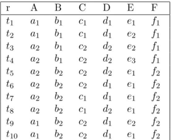
r A B C D E F t1 a1 b1 c1 d1 e1 f1 t2 a1 b1 c1 d1 e2 f1 t3 a2 b1 c2 d2 e2 f1 t4 a2 b1 c2 d2 e3 f1 t5 a2 b2 c2 d2 e1 f2 t6 a2 b2 c2 d1 e1 f2 t7 a2 b2 c1 d1 e1 f2 t8 a2 b2 c1 d2 e1 f2 t9 a1 b2 c2 d1 e2 f2 t10 a1 b2 c2 d1 e1 f2
Figure 1: An instance relation r of the schema R
A
Illustrative Example
We present an illustrative example to help the reviewer understanding our results. Due to lack of space, this example has been removed from the main paper. The different examples illustrate the different results and are all based on the relation of figure 1.
Example 1 (CFDs definition) The CFDϕ1 = (AB→C,{(⊤, b2,⊤,⊥,⊥,⊥)}) is not satisfied by the relation in figure 1 because of tuples t6 and t7.
However, the CFDs:
• ϕ2 = (AB→C,{(a1, b1, c1,⊥,⊥,⊥),(a2, b1, c2,⊥,⊥,⊥), (a1, b2, c2,⊥,⊥,⊥)})
• ϕ3 = (AB→C,{(a1,⊤,⊤,⊥,⊥,⊥),(⊤, b1,⊤,⊥,⊥,⊥)}) are satisfied by the relation. Note that ϕ2 and ϕ3 are equivalent in the relation. Indeed, the FD AB → C is satisfied in the fragment relation
rϕ2 = rϕ3 = {t1, t2, t3, t4, t9, t10} while it does not hold on the fragment relation r−rϕ2.
There are no CFDs of the form (AD→C, Tp) in the relation.
The FDs of the relation are {B → F, F → B, ACDE → BF, ACE →
BF}. ⋄.
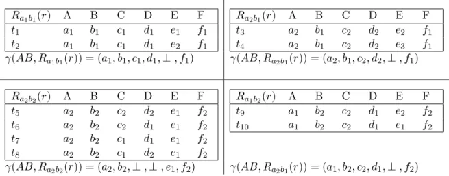
Example 2 (X-complete patterns) In the relation of figure 1, the frag-ment relation rAB ={t1, t2} is AB-complete. The AB-complete horizontal decomposition of r is RAB(r) = {{t1, t2},{t3, t4},{t5, t6, t7, t8},{t9, t10}}. This decomposition is shown on figure 2.
The set of AB-complete patterns is Γ(AB, r) ={(a1, b1, c1, d1,⊥, f1), (a2, b1, c2, d2,⊥, f1),(a2, b2,⊥,⊥, e1, f2),(a1, b2, c2, d1,⊥, f2)}.
Ra1b1(r) A B C D E F t1 a1 b1 c1 d1 e1 f1 t2 a1 b1 c1 d1 e2 f1 Ra2b1(r) A B C D E F t3 a2 b1 c2 d2 e2 f1 t4 a2 b1 c2 d2 e3 f1
γ(AB, Ra1b1(r)) = (a1, b1, c1, d1,⊥, f1) γ(AB, Ra2b1(r)) = (a2, b1, c2, d2,⊥, f1)
Ra2b2(r) A B C D E F t5 a2 b2 c2 d2 e1 f2 t6 a2 b2 c2 d1 e1 f2 t7 a2 b2 c1 d1 e1 f2 t8 a2 b2 c1 d2 e1 f2 Ra1b2(r) A B C D E F t9 a1 b2 c2 d1 e2 f2 t10 a1 b2 c2 d1 e1 f2
γ(AB, Ra2b2(r)) = (a2, b2,⊥,⊥, e1, f2) γ(AB, Ra2b1(r)) = (a1, b2, c2, d1,⊥, f2) Figure 2: TheAB-complete horizontal decomposition of relationr of figure
1 and their corresponding AB-complete patterns. The closure of AB is
θ(AB, r) ={A, B, F}.
The closure of AB is θ(AB, r) = {A, B, F}. Note that this is coherent with the FDB →F.
⋄.
Example 3 (Link between FDs, CFDs and ARs) The CFDϕ4 = (E →
A,{(a2,⊥,⊥,⊥, e3,⊥,}) is a pure AR of the relation of figure 1.
ϕ2 = (AB→C,{(a1, b1, c1,⊥,⊥,⊥),(a2, b1, c2,⊥,⊥,⊥),
(a1, b2, c2,⊥ ,⊥ ,⊥ )}) is a pure CFD of the same relation. Note that
AB→C is an AR in the fragment relationsRa1b1(r),Ra2b1(r)andRa1b2(r)
(see figure 2). In the same way,AB→Cis an FD for the fragment relation
rϕ2 =Ra1b1(r)∪Ra2b1(r)∪Ra1b2(r) ⋄.
Example 4 (Main results) Consider attributesAD of the relation in fig-ure 1.
Γ(AD, r) ={ (a1,⊥,⊥, d1,⊥,⊥),(a2, b2,⊥, d1, e1, f2), (a2,⊥,⊥, d2,⊥,⊥)}.
From this, we see that Ψ(AD → C) = ∅. As consequence, there are no CFDs inr of the form (AD→C, Tp).
Now consider attributes ACE.
Γ(ACE, r) ={ (a1, b1, c1, d1, e1, f1),(a1, b1, c1, d2, e2, f1), (a1, b2, c2, d1, e1, f2),(a1, b2, c2, d1, e2, f2), (a2, b2, c1,⊥, e1, f2),(a2, b2, c2,⊥, e1, f2), (a2, b1, c2, d2, e2, f1),(a2, b1, c2, d2, e3, f1)}
We have thusΨ(ACE 6→B) =∅. Thus,ACE →B is an FD of the relation. If we consider attributes AB we can check that Ψ(AB → C) 6= ∅ and Ψ(AB 6→ C) 6= ∅ (see figure 2). Thus, there exists a CFD of the form (AB→C, Tp) in r (it is the CFDϕ2 of the previous examples). ⋄.
Example 5 (Constraint satisfaction for pattern tableaux) Consider attributes ABC in the relation of figure 1.
Γ(ABC, r) ={ (a1, b1, c1, d1,⊥, f1),(a1, b2, c2, d1,⊥, f2), (a2, b1, c2, d2,⊥, f1),(a2, b2, c1,⊥, e1, f2), (a2, b2, c2,⊥, e1, f2)} We have: Ψ(ABC →D) ={ (a1, b1, c1, d1,⊥, f1),(a1, b2, c2, d1,⊥, f2), (a2, b1, c2, d2,⊥, f1)} and Ψ(ABC 6→D) ={ (a2, b2, c1,⊥, e1, f2),(a2, b2, c2,⊥, e1, f2)}. We thus obtain the following constraints:
C(ABC 6→D) = (A6=a2∨B 6=b2∨C 6=c1) ∧ (A6=a2∨B =6 b2∨C 6=c2) Considertp = (a1, b1, c1, d1,⊥, f1). We havetp(X) = (a1, b1, c1,⊥,⊥,⊥) rtp(Ψ(ABC 6→D)) ={ (⊥,⊥, c1,⊥,⊥,⊥), (⊥,⊥,⊥,⊥,⊥,⊥), (a1, b1, c1,⊥,⊥,⊥)}.
Minimal keys are (a1,⊥,⊥,⊥,⊥,⊥)and (⊥, b1,⊥,⊥,⊥,⊥). If we consider all pattern tuples inΨ(ABC →D), we finally obtain the following CFD:
ϕ5= (ABC →D,{{(a1,⊤,⊤, d1,⊥,⊥),(⊤, b1,⊤,⊤,⊥,⊥)}). Note thatϕ5 could be simplified since(A→D,{{(a1,⊥,⊥, d1,⊥,⊥)}) is a CFD ofr. ⋄.
Example 6 (Link between AFDs, ARs and approximate ARs) Consider the CFD:
ϕ2 = (AB→C,{(a1, b1, c1,⊥,⊥,⊥),(a2, b1, c2,⊥,⊥,⊥),
(a1, b2, c2,⊥ ,⊥ ,⊥ )}) of the relation in figure 1. The fragment relation satisfying the CFD ϕ2 is rAB→C = Ra1b1(r)∪Ra2b1(r)∪Ra1b2(r). Thus
|rAB→C |= 6. (see figure 2).
If we consider rAB6→C = Ra2b2(r), we could decompose it in ABC
-complete fragment relations: Ra2b2c1(r) ={t5, t6} and Ra2b2c2(r) ={t7, t8}. Each ABC-complete fragment relation satisfies the implication AB → C. We can thus add one of the fragment relation to rAB→C without
invalidat-ing AB →C. Both fragment relations have the same number of tuples: 2. Thus, the support of the AFD AB→C is 8. ⋄.
B
Proofs
The following appendices will not appear in the final paper. It is intended to ease the work of the reviewers.
Property 1 Let A6∈X. We have r X →A (i.e. X →A is an FD of r)
Proof ⇒: Let X → A be an FD of r. Consider theX-complete horizontal decomposition ofr. For anyr′∈RX(r) and∀t, t′ ∈r′, we havet[X] =t′[X].
And since X → A is an FD, t[A] =t′[A]. Thus, γ(X, r′)[A]6= ⊥. Hence,
A∈θ(X, r).
⇐: ConsiderA ∈ θ(X, A). Thus, ∀t, t′ ∈ r such that t[X] = t′[X], we have t[A] =t′[A] (since γ(X, rt)[A] 6=⊥). As a consequence, r X → A.
.
Proposition 1 Let r′ ⊆ r. Then r′ is X-complete if and only if r′ is
θ(X, r)-complete. Proof
⇐: trivial sinceX⊆θ(X, r).
⇒: Considert, t′ ∈ r′ such that t[X] =t′[X]. Let us demonstrate that
t[θ(X, r)] =t′[θ(X, r)].
∀A∈ θ(X, r)−X, r X →A (i.e. X → A is an FD). Thus, r′ X → A
sincer′⊆r. As a consequence,t[A] =t′[A]. .
Lemma 1 Let r be a relation, X ⊆ Attr(r), such that r is X-complete. Then the following assertions are equivalent:
1. (X→A, γ(X, r)) is a CFD of r
2. X→A is an FD of r
3. X→A is an AR of r
Proof If | r |= 1, the lemma trivially holds. We thus consider that
r contains at least two tuples t, t′. Since r is X-complete, we have r is
θ(X, r)-complete,RX(r) ={r}, and Γ(X, r) ={γ(X, r)}. IfA6∈θ(X, r), all
assertions are false (and thus equivalent). Suppose thatA∈θ(X, r). Thus,
∀t, t′ ∈r, we have t[X∪ {A}] =t′[X∪ {A}]..
Theorem 1 Let r a relation,X ⊆Attr(r),A∈Attr(r)\X andTp ={tp ∈
Γ(X, r)|tp[A]6=⊥ }. The following assertions are equivalent:
1. (X→A, Tp) is a CFD ofr
2. X→A is an FD of rTp
3. For any r′ ∈RX(rTp), X→A is an AR of r
′
Proof 1⇒2: We suppose that (X →A, Tp) is a CFD ofr. Thus,∀tp ∈Tp,
we havertp X→A. And since rTp =
S
tp∈Tprtp, we have rTpX→A. 2 ⇒ 3: We suppose that rTp X → A. We thus have ∀r
′ ∈ R
X(rTp),
r′ is X-complete. And since r′ X → A, r′ is X∪ {A}-complete. Hence, X→A is an AR ofr′.
3 ⇒ 1: We suppose that ∀r′ ∈ R X(rTp), X → A is an AR of r′. Thus r′ X → A. Since rT p = S r′∈R X(rTp)r ′, we have r Tp X →A. Moreover,
∀t′p ∈ Γ(X, r) such that t′p 6∈ Tp, we have t′p[A] =⊥ . Thus, rt′
p 6 X → A. And thusr−rTp 6X → A. We thus conclude that (X→ A, Tp) is a CFD ofr. .
Theorem 2 Givenr a relation,X ⊆Attr(r) and an attribute A6∈X. The dependency X → A is a functional dependency of r (i.e. A ∈ θ(X, r)) if and only if Ψ(X6→A) =∅.
Proof A∈θ(X, r)
⇔ ∀tp∈Γ(X, r), tp[A]6=⊥
⇔ Ψ(X→A) = Γ(X, r)
⇔ Ψ(X6→A) =∅. .
Theorem 3 Let r be a relation, X ⊆ Attr(r) and A 6∈ X. We have:
r(X→A,Ψ(X→A)) if and only if r (θ(X, r)→A,Ψ(X →A)).
Proof Trivial since rX→A=rθ(X,r)→A..
Theorem 4 Algorithm 2 computes all CFDs of the form (X →A, T) such that:
• ifT =T op(X∪ {A}) (i.e. it is an FD) then X is a minimal generator of θ(X, r);
• otherwise X =θ(X, r).
Proof Follows directly from Theorems 2 and 3..
Proposition 2 Ψ(X →A)⊆Γ(X∪ {A}, r).
Proof If Ψ(X → A) = ∅, the proposition is trivial. We consider that Ψ(X → A) 6= ∅. For all tp ∈ Ψ(X → A), we have t[A] 6= ⊥ .
More-over,t[A] =γ(X, rtp)[A] sincertp is γ(X, r)-complete andrtp X→A. As a consequence,rtp ∈RX∪{A}(r). Thus, Ψ(X →A)⊆Γ(X∪ {A}, r).
Theorem 5 Given r a relation and (X →A,Ψ(X →A))a CFD of r then for any model m of C(X6→A), the pair(X→A, m) defines a CFD of r. Proof Considerm a model of C(X6→A)
⇒ ∀tp∈Ψ(X6→A), m6⊑tp
⇒ ∀t∈rX6→A, m6⊑t
⇒ rm⊆rX→A
⇒ rmX→A
Proposition 3 Given a relation r, Ψ(X → A) and Ψ(X 6→ A), a pattern tuple m is a model of C(X 6→A) in r if and only if ∃tp ∈Ψ(X → A) and
∀t′p∈Ψ(X6→A) we have t′p6⊑m andm ⊑tp.
Proof A pattern tuplem is a model ofC(X6→A)
⇔ ∀tp∈Ψ(X6→A), m6⊏tp (by definition).
We consider Y ⊆X the attributes ofm which are not equal to ⊥.
m is of a model inr if and only if m is a model andrm6=∅.
⇔ ∃t∈rX→A,m⊆t ⇔ ∃t∈rX→A,m[Y] =t[Y] ⇔ ∃t∈rX→A,∃tp ∈Ψ(X→A),tp ⊏t and m[Y] =t[Y] ⇔ ∃t∈rX→A,∃tp ∈Ψ(X→A),tp[X] =t[X] andm[Y] =t[Y] ⇔ ∃t∈rX→A,∃tp ∈Ψ(X→A),tp[Y] =t[Y] =m[Y] (sinceY ⊆X) ⇔ ∃t∈rX→A,∃tp ∈Ψ(X→A),m⊑tp⊑t ⇔ ∃tp∈Ψ(X→A), m⊑tp .
Theorem 6 The pattern tuple mp defines a model of C(X 6→A) in r if
and only if there exists tp ∈Ψ(X →A) such that γ(mp, rtp(Ψ(X 6→A))) =
tp(X).
Proof mp model inr
⇔ ∀t′p∈Ψ(X6→A), mp 6⊑t′p and rm 6=∅
⇔ ∀t∈rtp(Ψ(X 6→A)) such thatt6=tp(X), mp 6⊑tand rm6=∅
⇔ γ(mp, rtp(Ψ(X6→A))) =tp(X) and rm6=∅ And since ∃t∈r such thattp(X)⊏t:
⇔ γ(mp, rtp(Ψ(X6→A))) =tp(X) . Proposition 4 Given a CFD (X→A, Tp): Support(X →A) =|rTp|+ X tp∈Ψ(X6→A) max({|r′ ||r′∈RA(rtp)})
Proof ∀tp ∈ Ψ(X 6→ A) and ∀r′ ∈ RA(rtp) we have r
′ X → A. Thus, rTp ∪r ′ X → A. Let r max = Stp∈Ψ(X6→A)r ′ such that r′ ∈ R A(rtp) and | r′ | is maximal. We thus have rTp ∪rmax X → A and for all
t∈(r−(rTp∪rmax)) we have (r−(rTp∪rmax))6X→A. As a consequence,Support(X →A) =|rTp∪rmax |..
Theorem 7 Support(X→A) = X r′∈RX(r) |r′tp | withr′ tp ∈RA(r ′) and(X→A, t
Proof ∀r′∈R
X(r) and∀r′′∈RA(r′) we have r′′X →A. ThusX →A is
an AR ofr′′ sincer′′ isX∪ {A}-complete.
Ifr′ =r′′ thenX →A is an AR of r′ with confidence 1,
Ifr′′⊂r′ thenX →A is an approximate AR ofr′ with confidence<1.
If |r′′ | is maximal in RA(r′), then the confidence of the approximate AR