Label Noise Reduction Without Assumptions

(1)

Dartmouth College

Dartmouth Digital Commons

Dartmouth College Undergraduate Theses

Theses and Dissertations

6-1-2020

Label Noise Reduction Without Assumptions

Jason Wei

Dartmouth College

Follow this and additional works at: https://digitalcommons.dartmouth.edu/senior_theses Part of the Computer Sciences Commons

Recommended Citation

Wei, Jason, "Label Noise Reduction Without Assumptions" (2020). Dartmouth College Undergraduate Theses. 164.

https://digitalcommons.dartmouth.edu/senior_theses/164

This Thesis (Undergraduate) is brought to you for free and open access by the Theses and Dissertations at Dartmouth Digital Commons. It has been accepted for inclusion in Dartmouth College Undergraduate Theses by an

(2)

Label Noise Reduction Without Assumptions

Jason Wei Undergraduate Thesis Department of Computer Science

Dartmouth College [email protected]

Advisor: Lorenzo Torresani

Dartmouth Computer Science Technical Report TR2020-899

Abstract

We propose an algorithm for training neural networks in noisy label scenarios that up-weighs per-example gradients that are more similar to other gradients in the same minibatch. Our approach makes no assumptions about the amount or type of label noise, does not use a held-out validation set of clean examples, makes relatively few computations, and only modifies the minibatch gradient aggregation module in a typical neural network training workflow.

For CIFAR-10 classification with varying levels of label noise, our method suc-cessfully up-weighs clean examples and de-prioritizes noisy examples, showing consistent improvement over a vanilla training baseline. Our results open the door to potential future work involving per-example gradient comparisons.

1 Introduction

In typical neural network training, the gradient for a given minibatch is computed by summing the gradients given by each example—in other words, each per-example gradient contributes equally to the gradient for the entire minibatch. While this setup works well and is commonly used in practice, based on human intuition, some examples might be more beneficial for training than others. In the vanilla training setting, it can be challenging to quantify exactly how and why some examples are better for training. In the noisy label setting, however, where not all data labels are correct, some examples—those with clean labels—are better for training by definition. How might we find and prioritize these clean examples?

Prior work has explored several approaches for discovering and up-weighing more important examples in both noisy label and general scenarios [1, 2, 3]. Although these approaches show substantive improvements, they often require a clean validation set and use complex methods such as meta-learning and reinforcement meta-learning. As such, their added utility with respect to their implementation, computation, and complexity costs can be relatively low for practical use.

In this work, we present a simple approach for finding and prioritizing clean examples in the noisy label scenario. In a given minibatch, we compare computed per-example gradients and up-weigh gradients that are more similar to other gradients in the minibatch. We emphasize several potentially appealing characteristics regarding the nature of our approach. First, our approach makes few assumptions about training setting, as it is agnostic to the type and amount of label noise as well as the network architecture used for training. Second, our approach does not require a held-out validation set of clean examples, which several previous methods [1, 3, 4] use to guide their data selection process. Finally, our algorithm performs few, parallelizable computations for comparing gradients, making minimal modifications that in theory could be packaged into a module that could easily be swapped in with current automatic differentiation libraries.

(3)

2 Proposed Method

When training neural networks in the noisy label scenario, some examples are labeled incorrectly and their gradients do not update the model towards the optimum weights with respect to some given evaluation set of clean labels. Therefore, the gradients produced by these examples are hurtful and less valuable for learning than gradients produced by correctly labeled examples.

We formulate an approach based on the intuition that good gradients will update the model weights more optimally and therefore will be more similar to each other compared with bad gradients. In other words, we expect the gradients from two correctly labeled examples to have high similarity, while the gradients from a correctly labeled example and an incorrectly labeled example should have low similarly. Based on this intuition, we hypothesize that gradients from correctly labeled examples will agree more with other gradients in the minibatch than gradients from incorrectly labeled examples, and we aim to up-weigh these correctly labeled examples. For instance, an example of an apple incorrectly labeled as an orange will produce a gradient that changes parameters to classify apples as oranges, which will likely differ substantially from both gradients of correctly labeled apples and those of correctly labeled oranges.

We express our algorithm formally as follows. In a minibatch ofmexamples, for each exampleiand its corresponding gradient∇i, we compute a weight

wi= X

j∈[m]\{i}

exp (D(∇i,∇j)) (1)

whereD(∇i,∇j)is the cosine similarity between∇iand∇j. After computingwifor alli∈[m], we normalize the per-example weights to sum to one by dividing eachwibyPiwi. Now, we output a new weighted minibatch gradient∇=P

iwi∇i, which is used to update the network.

Note that by definition, per-example gradients that are more similar to other gradients in the minibatch will have higherD(∇i,∇j)and therefore will be assigned higher weights, while gradients that are less similar to other gradients in the minibatch will have lower weights. We apply an exponential function toDbecause the cosine similarity between two gradients can be negative.

In practice, the following three simple modifications help generate higher quality weightings: 1. computingD(∇i,∇j)for only the values corresponding to the last layers of the network, 2. scalingD(∇i,∇j)by an annealing factorathat remains constant throughout training, and 3. computingwiusing only the top-kvalues ofD(∇i,∇j).

We explore the effects of these modifications in through ablation studies in§3.3.

3 Experiments

We perform several experiments in the noisy label scenario to compare our method with vanilla training. We use a similar setting to the UNIFORMFLIPexperiments in Ren et al. [3], where all labels in the training set can uniformly flip to any other label class (labels in the validation set remain clean), one of the most studied settings in the literature. We use the CIFAR-10 dataset [5], which contains 50,000 training images and 10,000 testing images uniformly distributed over ten classes. To save computation time, we use the LeNet architecture [6], a small five-layer neural network. For all experiments, we train LeNet with a minibatch size of 128 for 30 epochs with the Adam optimizer [7] at an initial learning rate of 0.001, decaying by 0.85 every epoch, with no hyperparameter tuning. 3.1 Main Result

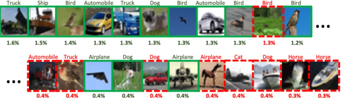
In Table 1, we show results for the CIFAR-10 dataset with 40% noise, comparing the performance of our proposed method with a vanilla training baseline as well as an idealoraclemethod that sets the weights of all incorrectly labeled examples to zero. For each configuration, we report the mean, standard deviation, and max over five random seeds where for each seed, we compute the mean validation accuracy during the last five epochs of training. The results for our proposed method shown here use the only last layer of gradients witha= 4andk= 4, enhancement parameters that we explore in 3.3. In Figure 1, we show an example ranking and weighitng from our method using the above configuration. In the next section, we elaborate more on relevant baselines for our experiment.

(4)

Training Algorithm Accuracy:µ±σ(max) Vanilla 55.65±0.75 (56.81) Oracle 62.31±0.87 (63.80) Ours 57.09±0.95 (58.43)

Table 1: For CIFAR-10 training with 40% label noise, our proposed method yields about 1% improvement over vanilla training.

Figure 1: Example ranking and weighting (highest and lowest weighted examples) from our proposed method using only the last layer of gradients with parametersa= 4andk= 4in a minibatch of 128 examples. Noisy labels are shown above each image and weights are shown below each image. Correctly labeled images are shown with solid green borders, whereas images with flipped labels labels have dashed red borders.

3.2 Baselines

As shown in Table 2, we also trained several natural baselines that address the noisy label setting, but do not find that they significantly improve over vanilla training. We find that the rectified Gaussian baseline [3] does not improve over vanilla training, which starkly contrasts the 7.9% improvement surprisingly reported by Ren et al. (keeping in mind that our experiments use a much smaller network than theirs). We also train a random-uniform baseline, where each per-example weight is uniformly sampled from(0,2/m), wheremis the minibatch size. This baseline does comparable with or worse than vanilla training.

As another set of baselines, we also explore a two-stage training scheme. We first train a vanilla model on noisy examples (as in the vanilla training baseline), and we either (1) fine-tune the same vanilla model using only examples where the potentially noisy label matches the model’s prediction (fine-tune), or (2) train a second model from scratch using only examples where the potentially noisy label matched the first model’s prediction (from scratch). Neither of these models outperform the vanilla training baseline. We train all baselines for 60 total epochs, compared with 30 epochs of training in the vanilla configuration.

Baseline Last-5 Acc Top-5 Acc

Vanilla 55.7 56.4

Rectified Gaussian 55.1 55.3 Uniform Random 55.8 56.0 Two-stage: Fine-Tune 49.8 49.8 Two-stage: From Scratch 52.9 53.0

Table 2: Baseline methods for addressing the label-noise scenario did not improve substantially over vanilla training despite being trained for twice as many epochs.

(5)

3.3 Ablation Studies

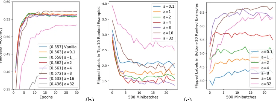
In this subsection, we explore three modifications to our method that help rank correctly labeled examples higher and incorrectly labeled examples lower, therefore leading to better performance. Similarity between different layers of gradients. Prior work has found that different layers in a neural network specialize in detecting specific features; for instance, the first layer of a neural network often focuses on low-level features that resemble Gabor filters or color blobs [8], while the last layers in a neural network often recognize high-level, task-specific features. As shown in Figure 2, we find that restricting the gradient similarity computation to only the last layer leads to better example rankings, since the last layer of a gradient likely relates more to the class of the example than earlier layers.

(a) (b) (c)

Figure 2: Restricting gradient similarity computations to only the last layer of the gradient yields better example rankings. (a) shows the training plot with the average validation accuracy over the last five epochs in brackets, (b) shows the number of incorrectly labeled examples in the top-10 examples by ranking (lower is better), and (c) shows the number of incorrectly labeled examples in the bottom-10 examples by ranking (higher is better).

ScalingD(∇i,∇j)by an annealing constanta. When using the cosine similarity function, the maximum agreement between two gradients is at most 1, and so even when two gradients are very similar, the signal from that pair is at most 1 and can be lost in the noise from a large number of gradient pairs in the minibatch that agree somewhat. In an attempt to address this issue, we scale D(∇i,∇j)by an annealing constantabefore applying the exponential function, which has the effect of up-weighing gradient pairs that with high similarity and down-weighing gradient pairs with weak or negative similarity.

(a) (b) (c)

Figure 3: Scaling theD(∇i,∇j)by an annealing constantaimproves example rankings, witha= 8 giving the best results. (a) shows the training plot with the average validation accuracy over the last five epochs in brackets, (b) shows the number of incorrectly labeled examples in the top-10 examples by ranking, and (c) shows the number of incorrectly labeled examples in the bottom-10 examples by ranking.

(6)

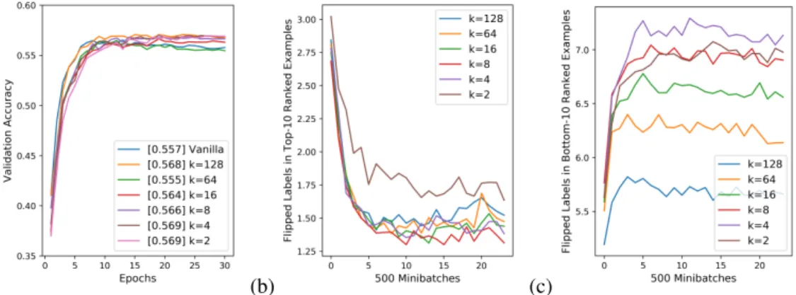
Computingwi using the only top-k D(∇i,∇j)values. In the original version of our algorithm, we computewiby summingexp(D(∇i,∇j))for allj∈[m]\{i}. It is possible, however, that not all other examplesjare relevant for determining whetheriis correctly labeled. We hypothesize that computingwiusing only the top-kvalues ofD(∇i,∇j)could yield a better ranking, since correctly labeled examples are expected to have several high values ofD(∇i,∇j)from other examples in their class, whereas incorrectly labeled examples should struggle to find other examples that produce high D(∇i,∇j). Figure 4 shows an ablation study fork={128,64,16,8,4,2}in the setting of 10-class classification with minibatch size 128 when the annealing constant is 4, and we see thatk = 4

produces the best results. An alternative modification could compare∇iand∇jonly wheniandj belong to the same class, but we find that this setup does not perform better than top-kweighting (see

§6.1).

(a) (b) (c)

Figure 4: Computingwiusing only the top-kvalues ofD(∇i,∇j)substantially improves ranking, withk = 4giving the best results for our scenario. (a) shows the training plot with the average validation accuracy over the last five epochs in brackets, (b) shows the number of incorrectly labeled examples in the top-10 examples by ranking, and (c) shows the number of incorrectly labeled examples in the bottom-10 examples by ranking.

3.4 Noising Ratios

As further analysis, we study how our proposed method performs compared with vanilla training for different noisy label ratios. Happily, we find that in addition to the 40% label noise scenario (60% clean data) used for all above experiments, our method also outperforms vanilla training for clean label ratios of 20%, 40%, and 80%. Figure 5 shows these results.

Figure 5: Our method is robust to the amount of label noise, outperforming vanilla training for clean label ratios of 20%, 40%, 60%, and 80%.

(7)

3.5 Decoupling Ranking and Weighting

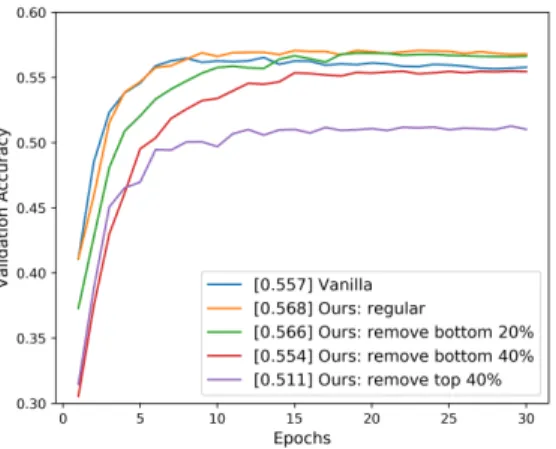
Our proposed algorithm provides both a ranking and weighting for the per-example gradients, but the algorithm that produces the best ranking may not produce the best weighting. In this experiment, we decouple ranking and weighting by using our proposed algorithm for ranking and using the following heuristic for weighting: some fraction of per-example gradients are removed (their weight is set to 0), and the remaining gradients are given uniform weight (such that the sum of their weights is 1). In Figure 6, we show results from removing the bottom-ranked 20% and 40% gradients, for which removing the bottom 20% of gradients outperforms vanilla training. As additional confirmation of signal in the ranking produced by our method, we show that removing the top-ranked 40% gradients does considerably worse, as expected.

Figure 6: Results when our proposed algorithm is used purely for ranking and weighting is done by removing some of the per-example gradients in the minibatch and giving the remaining gradients uniform weight. Average validation accuracy over the last five epochs is shown in brackets.

4 Related Work

Several prior studies have proposed methods for weighting training examples differently. Perhaps the two most relevant are Ren et al. [3] and Wang et al. [1]. Ren et al. proposed a meta-learning algorithm that assigns per-example weights to minimize the loss on a clean unbiased validation set via a meta-learning algorithm, showing substantial improvements in data imbalance and noisy label scenarios [3]. In the same spirit, Wang et al. up-weighed examples with similar gradients to a validation set using reinforcement learning and demonstrated improvements for both image classification and machine translation [1]. These studies both show strong results but use a held-out validation set to guide optimization, which we do not use.

Our work also draws inspiration from work in the area of curriculum learning [9], which also aims to present data to models in a non-uniform fashion but in terms of order instead of weighting. In curriculum learning, heuristics are often used to gain insight into which examples might be more meaningful (often in terms of easy and hard) [10, 11, 12, 13], while our method uses gradient similarity to determine how to weigh examples. Boosting algorithms such as AdaBoost [14], which selects harder examples for training subsequent classifiers, also relate to our work in a similar fashion. The noisy label setting has been well-explored in deep learning literature in many methods that do not modify how per-example gradients are aggregated. Hendrycks et al. [4] use a loss correction technique that uses trusted examples to mitigate label noise; Jiang et al. [15] train a mentor network to provide a curriculum for a student network to focus on samples of labels that are probably correct; Li et al. [16] present a distillation framework evaluated on several real-world datasets; Menon et al. [17] propose a variation of gradient-clipping; and Xiao et al. [18] use a probabilistic graphical model to correct wrong labels in a clothing classification dataset. While these methods all provide substantive improvements over vanilla training, they use (understandably) complex methods that sometimes involve multiple stages of training, whereas our method makes minimal modifications to standard neural network training.

(8)

Finally, computing per-example gradients is required for implementing our method, a non-trivial implementation detail not native to automatic differential libraries, for which [19, 20] are helpful resources.1

5 Discussion

In closing, we have shown that in the noisy label scenario, up-weighing per-example gradients that are more similar to other gradients in the same minibatch produces a ranking that prioritizes clean examples and leads to better training in the noisy label scenario. Our findings indicate some signal in the idea of comparing per-example gradients, opening the door to future work along similar lines. Our approach, however, does have limitations. Foremost, we found in preliminary experiments that using our method for the clean data setting can produce either an improvement or a decay in performance of up to 1%, depending on the task and the parameters used for our algorithm.2 Further experiments will need to be conducted to find parameters for our algorithm that provide both substantive improvement on the noisy label scenario and non-inferior performance in the clean data scenario. Also, while our parameters for top-kand annealing appear relatively robust in our experiments, it might be necessary to tune those parameters when training with particularly small or large minibatch sizes and for different noising ratios.

Future work could take several directions. In the noisy label scenario, we could enhance our algorithm to fix the label of examples likely to be incorrect, potentially by making comparisons of gradients computed with hypothetical labels. In the general scenario, our algorithm could be seen as a type of momentum, for which we have seen some promising results but would need further parameter tuning and experiments to confirm. For additional evaluation, our method could be validated in other settings such as the real-world datasets proposed by Li et al. [16], weakly labeled datasets [21], or noisy label scenarios in natural language processing (as our technique is not specific to computer vision). Finally, to facilitate use of our algorithm as an easy-to-use baseline over vanilla training, we could refactor our existing code as PyTorch module for easy implementation by other researchers.

Acknowledgements

Jason Wei thanks Lorenzo Torresani for exceptional advising and support. We thank Yiren Jian for general coding pointers and references to implementations of per-example gradient computations.

1

https://github.com/cybertronai/autograd-hacksgives per-example gradients in PyTorch. 2

In preliminary experiments, we found our method to give 1% improvement on CIFAR-100 and 1% decrease in performance on CIFAR-10 in the clean data scenario.

(9)

References

[1] Xinyi Wang, Hieu Pham, Paul Michel, Antonios Anastasopoulos, Graham Neubig, and Jaime G. Carbonell. Optimizing data usage via differentiable rewards. ArXiv, abs/1911.10088, 2019. https://arxiv.org/abs/1911.10088.

[2] Angelos Katharopoulos and François Fleuret. Not all samples are created equal: Deep learning with importance sampling. InInternational Conference on Machine Learning (ICML), 2018. https://arxiv.org/abs/1803.00942.

[3] Mengye Ren, Wenyuan Zeng, Bin Yang, and Raquel Urtasun. Learning to reweight examples for robust deep learning. InInternational Conference on Machine Learning (ICML), 2018. https://arxiv.org/abs/1803.09050.

[4] Dan Hendrycks, Mantas Mazeika, Duncan Wilson, and Kevin Gimpel. Using trusted data to train deep networks on labels corrupted by severe noise. In Proceedings of the 32nd International Conference on Neural Information Processing Systems (NIPS), 2018. https: //arxiv.org/abs/1802.05300.

[5] Alex Krizhevsky. Learning multiple layers of features from tiny images. University of Toronto, 2012.https://www.cs.toronto.edu/~kriz/learning-features-2009-TR.pdf. [6] Yann LeCun, Léon Bottou, Yoshua Bengio, and Patrick Haffner. Gradient-based learning

applied to document recognition.Proceedings of the IEEE, 86(11):2278–2324, 1998.https: //ieeexplore.ieee.org/document/726791.

[7] Diederik Kingma and Jimmy Ba. Adam: A method for stochastic optimization. International Conference on Learning Representations (ICLR), 2014. https://arxiv.org/abs/1412. 6980.

[8] Jason Yosinski, Jeff Clune, Yoshua Bengio, and Hod Lipson. How transferable are features in deep neural networks? InAdvances in Neural Information Processing Systems 27 (NIPS). 2014. https://arxiv.org/abs/1411.1792.

[9] Yoshua Bengio, Jérôme Louradour, Ronan Collobert, and Jason Weston. Curriculum learning. InInternational Conference on Machine Learning (ICML), 2009.http://doi.acm.org/10. 1145/1553374.1553380.

[10] Yulia Tsvetkov, Manaal Faruqui, Wang Ling, Brian MacWhinney, and Chris Dyer. Learning the curriculum with Bayesian optimization for task-specific word representation learning. In

Proceedings of the 54th Annual Meeting of the Association for Computational Linguistics (Volume 1: Long Papers).https://www.aclweb.org/anthology/P16-1013.

[11] Alex Graves, Marc G. Bellemare, Jacob Menick, Rémi Munos, and Koray Kavukcuoglu. Automated curriculum learning for neural networks. International Conference on Machine Learning (ICML), 2017. http://proceedings.mlr.press/v70/graves17a/graves17a. pdf.

[12] Daphna Weinshall and Gad Cohen. Curriculum learning by transfer learning: Theory and experiments with deep networks. InInternational Conference on Machine Learning (ICML), 2018.https://arxiv.org/abs/1802.03796.

[13] Guy Hacohen and Daphna Weinshall. On the power of curriculum learning in training deep networks. InInternational Conference on Machine Learning (ICML), 2019. https://arxiv. org/abs/1904.03626.

[14] Yoav Freund and Robert Schapire. A short introduction to boosting.Journal-Japanese Society For Artificial Intelligence, 14(771-780):1612, 1999.https://cseweb.ucsd.edu/~yfreund/ papers/IntroToBoosting.pdf.

[15] Lu Jiang, Zhengyuan Zhou, Thomas Leung, Li-Jia Li, and Li Fei-Fei. Mentornet: Learning data-driven curriculum for very deep neural networks on corrupted labels. InInternational Conference on Machine Learning (ICML), 2018. http://proceedings.mlr.press/v80/ jiang18c/jiang18c.pdf.

(10)

[16] Yuncheng Li, Jianchao Yang, Yale Song, Liangliang Cao, Jiebo Luo, and Jia Li. Learning from noisy labels with distillation. In2017 IEEE International Conference on Computer Vision (ICCV), pages 1928–1936, 2017.http://openaccess.thecvf.com/content_ICCV_2017/ papers/Li_Learning_From_Noisy_ICCV_2017_paper.pdf.

[17] Aditya Krishna Menon, Ankit Singh Rawat, Sashank J. Reddi, and Sanjiv Kumar. Can gradient clipping mitigate label noise? InInternational Conference on Learning Representations (ICLR), 2020.https://openreview.net/forum?id=rklB76EKPr.

[18] Tong Xiao, Tian Xia, Yi Yang, Chang Huang, and Xiaogang Wang. Learning from massive noisy labeled data for image classification. In2015 IEEE Conference on Computer Vision and Pattern Recognition (CVPR), pages 2691–2699, 2015.http://openaccess.thecvf.com/ content_cvpr_2015/papers/Xiao_Learning_From_Massive_2015_CVPR_paper.pdf. [19] Ian J. Goodfellow. Efficient per-example gradient computations. ArXiv, abs/1510.01799, 2015.

https://arxiv.org/abs/1510.01799.

[20] Gaspar Rochette, Andre Manoel, and Eric W. Tramel. Efficient per-example gradient computations in convolutional neural networks. ArXiv, abs/1912.06015, 2019. https: //arxiv.org/abs/1912.06015.

[21] Zhi-Hua Zhou. A brief introduction to weakly supervised learning. National Science Review, 5:44–53, 2018. https://academic.oup.com/nsr/article-pdf/5/1/44/31567770/ nwx106.pdf.

(11)

6 Supplementary Materials

6.1 Computingwiusing only within-classD(∇i,∇j)

A natural idea is to computewiusing onlyD(∇i,∇j)wheniandjbelong to the same class, since correctly labeled examples should have high similarity with other correctly labeled examples, whereas incorrectly labeled examples should not have high similarity with any other examples in the same supposed class. We find that, as shown in Figure 7, this method helps does not outperform top-k weighting for our setting. Notably, the intuition of this within-class idea is only valid when there are a large number of examples per class in each minibatch.

(a) (b) (c)

Figure 7: Computingwiusing only within-classD(∇i,∇j)does not outperform the top-k modifi-cation. (a) shows the training plot with the average validation accuracy over the last five epochs in brackets, (b) shows the number of incorrectly labeled examples in the top-10 examples by ranking, and (c) shows the number of incorrectly labeled examples in the bottom-10 examples by ranking.