FACULTY OF BUSINESS STUDIES
DEPARTMENT OF ACCOUNTING AND FINANCE
Hoa Dang Doan Thien
EVALUATION OF VOLATILITY FORECASTING MODELS IN VIETNAM STOCK MARKETS
Master’s Thesis in Accounting and Finance
Finance
TABLE OF CONTENTS
1. INTRODUCTION 11
1.1. Purposes of the study 13
1.2. Structure of the thesis 14
2. VOLATILITY 15
2.1. What is Volatility? 15
2.2. Unconditional Variance - Conditional Variance 15
2.3. Stylized Facts about Asset Price Volatility 16
2.3.1.Volatility Clustering 16
2.3.2.Mean Reversion 17
2.3.3.Asymmetric Response 17
2.3.4.Long Memory 17
2.3.5.Influenced by Exogenous Variables 18
2.3.6.Fat Tail Distribution 18
3. VOLATILITY FORECASTING 20
3.1. Volatility Forecast Models 20
3.1.1.Basic notation 20
3.1.2.Exponentially Weighted Moving Averages (EWMA) – RiskMetrics
EWMA 22
3.1.3.Generalized Autoregressive Conditional Heteroskedasticity
3.1.4.Exponential GARCH - EGARCH 24
3.1.5.GJR-GARCH 25
3.1.6.Integrated GARCH – IGARCH 25
3.1.7.Fractionally Integrated GARCH - FIGARCH 26
3.1.8.Asymmetric Power ARCH - APARCH 27
3.2. Volatility Forecast Evaluation 28
3.2.1.Symmetric Loss Functions 29
3.2.2.Asymmetric Loss Function 30
3.2.3.Test for Superior Predictive Ability (SPA) 31
3.2.4.Model Confidence Set (MCS) 32
3.2.5.Value-at-Risk forecasts 34
4. PREVIOUS EMPIRICAL STUDIES 36
5. DATA COLLECTION AND METHODOLOGY 40
5.1. Data Collection 40
5.2. Methodology 41
6. EMPIRICAL RESULTS 45
6.1. Preliminary Data 45
6.2. Symmetric Forecast Error Measures 48
6.3. Asymmetric Forecast Error Measures 52
6.4. Superior Predictive Ability Test Results 55
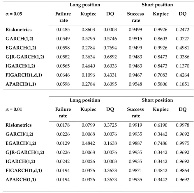
6.6. VaR forecast evaluation 58
7. SUMMARY AND CONCLUSION 62
BIBLIOGRAPHY 66
APPENDIX 1 75
LIST OF TABLES
Table 1: The equations of studied volatility models ...43
Table 2: Unit root tests ...45
Table 3: Ljung-Box test statistics ...46
Table 4: Descriptive statistics of the residual series ...47
Table 5: ARCH Lagrange Multiplier test statistics ...47
Table 6: Descriptive statistics of proxied “true” volatility series ...48
Table 7: Relative forecast error statistics ...50
Table 8: Ranks of symmetric error statistics ...51
Table 9: Mean mixed error and numbers of under- and over-predictions ...54
Table 10: Summary of SPA test results ...56
Table 11: Model Confidence Set ...57
UNIVERSITY OF VAASA Faculty of Business Studies
Author: Doan Thien Hoa Dang
Topic of the Thesis: Evaluation of Volatility Forecasting Models in Vietnam Stock Markets
Name of the Supervisor: Professor Janne Äijö
Degree: Master of Science in Economics and Administration
Department: Department of Accounting and Finance Major Subject: Accounting and Finance
Line: Finance Year of Entering the University: 2009
Year of Competing the Thesis: 2011 Pages: 80
ABSTRACT
This study aims to find the most appropriate model(s) to estimate and forecast volatility in Vietnam stock markets. Considered volatility models in this study include RiskMetrics, GARCH, EGARCH, IGARCH, FIGARCH and APARCH. The forecast performance evaluations are conducted with two Vietnam stock indices – VNI-index and HNX-index. Selected data periods is from 01 March 2002 to 30 June 2011 for VNI-index and the period for HNX-index spans from 01 June 2006 through 30 June 2011. Symmetric loss functions and asymmetric loss functions are used as basic analysis criteria. Robust conclusions are achieved with the superior predictive ability (SPA) test, the model confidence set (MCS) procedure and Value-at-Risk (VaR) forecast evaluation.
The general empirical results generated from symmetric loss functions, the SPA test and the MCS procedure demonstrate that for VNI-index, RiskMetrics and EGARCH have equally best forecast performance while for HNX-index, only EGARCH has the best. However, there are contrast findings resulted from different assessment criteria specifically with asymmetric loss functions and VaR forecast. Actually, the ranking of models is sensitive to the selected criterion. Therefore, selecting reasonable evaluation criteria is very critical and it must be established on the ultimate aims of the forecasting procedure.
1. INTRODUCTION
Volatility is an unobservable process, thus its value can only be estimated by specific models. There are many important applications of volatility in different financial activities for instance in risk management, assets allocation, derivatives valuation, hedging and policy making. Moreover, in these applications, future values of volatility are typically required. Therefore, the forecasting powers of volatility models have attracted concerns of both academic researchers and practitioners. Many previous studies were conducted to evaluate the forecast performance of different models. Nevertheless, different empirical data and varied evaluating criteria gave inconsistent results.
Vietnam, one of the newest emerging markets in Asia, is still not so popular to the world’s perception. Moreover, its stock market was just established in year 2000. Thus few research papers could employ empirical data of this market. On the other hand, the demand of studies about Vietnam stock market’s volatility has been increasing because of following reasons. The regulations for stock market operations are imperfect and incomplete. Investors have to consider seriously this legal risk and they account it into the stocks’ prices. Besides, Vietnam stock market has expanded its scale dramatically in years in substantial spread. It also has experienced the world financial crisis since 2008. Hence movement of this stock market has been very volatile.
The above-mentioned facts really have frustrated investors and also policy makers. Choosing precise, effective, feasible and practical volatility models in this specific market is a critical and essential issue. However, to the best of my knowledge, there is no paper studying about forecast performance of volatility models in this market.
There are two main approaches in volatility forecasting models (Poon & Granger 2003: 482). The first one uses historical data to formulate the models to predict future volatility. The second one calculates estimated volatility from options’ prices. However, the second method is not applicable in this market because there is no option market presently in Vietnam. Therefore in this study, forecasting performance of models adopting the first approach is concentrated.
In the group using historical information set to forecast, there are three subcategories including models based on past standard deviation which are normally known as simple historical models, Autoregressive Conditional Heteroskedasticity (ARCH) class conditional volatility models and stochastic volatility models (Poon & Granger 2003: 483 - 486). Even though stochastic volatility models have been attracted many academics with vast literature (Poon & Granger 2003; Andersen, Bollerslev, Christoffersen & Diebold 2006), it is still not very popular in practical industry.
The concerned models for this study are those which are familiar and feasible to apply in practice. The most popular and widely used model represents for the group based on past standard deviation is the RiskMetrics Exponentially Weighted Moving Averages (EWMA) model. While in the ARCH family, GARCH and several other GARCH-genre models such as EGARCH, AGARCH, GJR-GARCH and many others are also very well-known in applications. In this paper, selected models to evaluate include of RiskMetrics EWMA, GARCH, EGARCH, GIR-GARCH, IGARCH, FIGARCH and APARCH.
1.1. Purposes of the study
Even though GARCH and GARCH-genre models are expected to outperform the simple historical models because these models are formulated to capture specific characteristics of volatility, the empirical results in previous studies do not totally support this perspective. There are still some evidences preferring the simple historical to GARCH approach models (Cumby, Figlewski, & Hasbrouck 1993; Figliewski 1997). Thus, in reality, GARCH genre models are not always the most suitable to apply.
In the latest study relating to volatility forecast power comparison, McMillan and Kambouroudis (2009) compare the RiskMetrics EWMA model, GARCH and other GARCH genre models with empirical data from 31 stocks markets including G7 countries, 13 countries in Europe and 11 countries in Asia. They conclude that the RiskMetrics model is appropriate in most Asian markets while the APARCH model performs better in the G7, the Europe markets and the larger Asian markets. Nevertheless, Vietnam is not included in this study. Hence, this study is conducted to evaluate the volatility forecasting performance of the current popular models consisting of the RiskMetrics EWMA, GARCH and several other popular GARCH genre models in Vietnam stock markets. Based on the conclusion of McMillan and Kambouroudis (2009), the RiskMetrics EWMA model is expected to have the most forecasting power in Vietnam stock markets. Therefore, in this study, it is considered as the benchmark model and the following main hypothesis is going to be tested.
H1: RiskMetrics EWMA model provides better volatility forecasts than other considered GARCH type models in Vietnam stock markets.
There are two main aims of this study. The first one is to assess the volatility forecasting performance of different popular models in Vietnam stock market, specifically with two indices VNI-index and HNX-index. Hence, the applicable model is found out to apply in practice. The second target is that the empirical result of this study will augment to the results of previous studies and contribute more empirical results to the literature relating to this research topic.
1.2. Structure of the thesis
The remained content of the thesis is organized as following. Chapter two and chapter three cover the essential theoretical framework relating to the research issue. Chapter two describes the financial volatility concept and its common stylized facts. The next chapter introduces concerned volatility estimation and forecasting models. It also explains the forecast evaluation procedure including basic evaluation from loss functions, superior predictive ability test for robust conclusion, model confidence set procedure as well as Value-at-Risk back-test. Chapter four reviews several main papers relating to forecast performance comparison between different models. Moreover, chapter five describes briefly data collection and the methodology applied in this study while chapter six reports the empirical results. Finally, summary of the study and the conclusion with suggested ideas for further research are presented in chapter seven.
2. VOLATILITY
2.1. What is Volatility?
Within economics, volatility terminology is used to define the variability of the random component of a time series (Andersen et al. 2006: 780). More precisely in finance, Alexander (2008: 90) gives the definition of the volatility of an asset as “an annualized measure of dispersion in the stochastic process that is used to model the log returns”. Andersen et al. (2006: 780) express this term even more specifically as “the instantaneous standard deviation of the random Wiener-driver component in a continuous–time diffusion model”.
Moreover, volatility commonly refers to the standard deviation σ or variance σ2 which represent the second moment characteristic of the sample and measure the dispersion about the mean of the distribution (Poon & Granger 2003: 480; Alexander 2008: 90). In this study, volatility term is utilized in this conception.
2.2. Unconditional Variance - Conditional Variance
In the literature on estimating and forecasting volatility, it is very important to understand the differences between conditional variance and unconditional variance. The brief comparison of these terms given by Alexander (2008) presented below illustrates the apparent distinction between the two concepts.
The unconditional variance is just the variance of the unconditional returns distribution, which is assumed constant over the entire data period considered.
The conditional variance, on the other hand, will change at every point in time because it depends on the history of returns up to that point.
(Alexander 2008: 131-132)
The unconditional variance is considered as long term average variance whereas the conditional variance is the instantaneous variance with inconstant value (Alexander 2008).
2.3. Stylized Facts about Asset Price Volatility
Financial asset price volatility has some specific characteristics which were observed and confirmed in vast literature. The existence of a lot of volatility models is mainly caused by the expectation to capture these properties to provide the best estimation and forecast. It is important to know these features before coming to the volatility models in the next section.
2.3.1. Volatility Clustering
Volatility clustering feature is first reported by Mandelbrot (1963) and then is confirmed in numerous later studies (Fama 1965; Chou 1988; Schwert 1989). It is described as large changes in the price of an asset tend to be followed by large changes and small changes tend to be followed by small changes. This property implies that volatility shocks today will influence the expectation of future volatility in many periods (Engle & Patton 2001). The ARCH model first suggested by Engle (1982) to capture this behavior became a foundation for developments of numerous ARCH genre models.
2.3.2. Mean Reversion
This property of volatility means that volatility will eventually return to the mean level, which is the long term average volatility (Engle & Patton 2001; Alexander 2008). Engel and Patton (2001) state that all long run forecasts of volatility should all converge to this level, no matter when they are made. It also implies that very long run forecast is not affected by current shock.
2.3.3. Asymmetric Response
The equity market volatility is not affected symmetrically by positive and negative return shocks. This feature is also known as leverage effect because as stock price decreases debt-to-equity ratio increases thus leads to highly leveraged firm and consequently rises the volatility. In contrast, as stock price increases by a same amount, volatility does not change with the same magnitude but smaller one. (Engle & Patton 2001; Andersen et al. 2006; Alexander 2008)
Several GARCH genre models have been proposed to capture this asymmetric response including but not limited to AGARCH (Engle & Ng 1993), EGARCH (Nelson 1991), GJR-GARCH (Glosten, Jagannathan & Runkle 1993) or TGARCH (Zakoïan 1994).
2.3.4. Long Memory
According to Poon (2005), long memory in volatility is the phenomenon that the autocorrelation of measures of volatility for instance absolute or squared
returns decay slowly at a hyperbolic rate. The presence of this feature is reported in several studies (Ding, Granger & Engle 1993; Dacorogna, Müller, Nagler, Olsen & Pictet 1993; Anderson & Bollerslev 1997).
The GARCH, AGARCH, EGARCH and GJR-GARCH models imply an exponential decay in the autocorrelation of conditional variances. Hence, several GARCH approach models have been proposed to handle this long memory effect for example IGARCH of Engel and Bollerslev (1986) and FIGARCH of Baillie, Bollerslev and Mikkelsen (1996).
2.3.5. Influenced by Exogenous Variables
This stylized fact presents that different assets and different markets tend to have co-movements in the returns and volatilities (Engle, Ito & Lin 1990; Theodossiou & Lee 1993; Koutmos & Booth 1995; Koutmos 1996; Knif & Pynnönen 1999). Moreover, there are plenty of variables that correlate to movements of returns and volatilities for example bid-ask spread (Bollerslev & Melvin 1994), trading volume (Bollerslev & Jubinski 1999), macro announcement (Andersen & Bollerslev 1998b; Flannery & Protopapadakis 2002; Bomfim 2003) and even investors’ behaviours (Odean 1997; Castaldo, 2002; Gabaix, Gopikrishnan, Plerou, & Stanley 2006).
2.3.6. Fat Tail Distribution
Empirical data in literature on financial asset returns illustrates that distributions of asset returns are not normal but fatter tails and more kurtosis than those are predicted by normal distribution (Mandelbrot 1963; Fama 1963,
1965; Blattberg & Gonedes 1974). This feature indicates that assets’ returns are not independent and identically distributed as in assumption normally using in various financial applications. The appropriate volatility models should capture this property properly.
3. VOLATILITY FORECASTING
3.1. Volatility Forecast Models
Following the work of McMillan et al. (2009), in this study, forecast models are considered including RiskMetrics EWMA, GARCH and other GARCH-genre models such as EGARCH, IGARCH, GJR-GARCH, APARCH, and FIGARCH.
In the group of models which simply based on past standard deviation, simple historical models consisting of random walk, historical mean, moving average, exponential smoothing and simple regression models are not evaluated in this paper. Even though they are very simple and easy to apply, their extreme simplicities also make them unable to describe many critical properties of volatility process. Only Exponentially Weighted Moving Averages (EWMA) with its representative RiskMetrics EWMA model is assessed because of its advance and popularity in practical financial applications.
In the GARCH family models, each model with its own feature created to capture each specific characteristic of volatility is selected to evaluate in this study.
3.1.1. Basic notation
Let pt denotes the price of an asset at time t, the return on the asset over the
(1) r = lnp − lnp
The return series is modeled as following process:
(2) r = x′β+ u
u | ℱ ~ N0,σ
With xt is the set of independent variables affecting the conditional mean of rt
and ut is the error term, ℱ is the information set while is the conditional
variance of ut process.
The time-varying conditional mean and conditional variance of the return process are denoted as:
(3) µ =µ|= E[r | ℱ] (4) σ = σ | = Var[r|ℱ] = E[r−µ | |ℱ] = E[u |ℱ] Moreover, the unconditional mean and unconditional variance of the return series are also defined as:
(5) µ= E[r]
3.1.2. Exponentially Weighted Moving Averages (EWMA) – RiskMetrics EWMA
The EWMA one-day ahead variance and volatility are forecasted using following formulas with smoothing constant λ, and 0 < λ < 1.
(7) σ| = 1 − λ !λ" ∞ "#$ r" = 1 − λr+ λσ | (8) σ| = %1 − λr+ λσ|
There is not precise criterion to decide value of λ. It is normally chosen subjectively with value in the range from 0.75 to 0.98 (Alexander 2008: 122). In the RiskMetrics EWMA of J.P. Morgan, daily return series use λ = 0.94, while monthly return series apply λ = 0.97 (RiskMetricsTM – Technical Document 1986).
Multiple-day horizon, over T-day period from day t, forecast of the variance using EWMA is:
(9) σ&'| = Tσ&|
The critical problem of this model is that volatility process is assumed to be constant. The volatility forecast is all the same for all the time horizons, which is equal to the current estimate. Thus, it is not able to forecast the long-term volatility. Moreover, the subjective decision for λ value is also a potential issue affecting the accuracy in forecast application. (Alexander 2008: 124). In addition,
this approach is also incapable to capture the asymmetric response and mean-reversion properties of asset return volatility (McMillan & Kambouroudis 2009: 118).
On the other hand, RiskMetrics model still has advantages that facilitate its popularity in practice. Firstly, it is convenient to track day-to-day volatility change. Secondly, moderate amount of data is required with simple calculations. Thirdly, the only unknown variable, λ, is not required to estimate. Its value has already been assigned. (McMillan & Kambouroudis 2009: 118)
3.1.3. Generalized Autoregressive Conditional Heteroskedasticity -GARCH
GARCH(p,q) model, generalized the ARCH model of Engle (1982), is proposed by Bollerslev (1986) to capture the volatility clustering.
(10) σ = ω+ !β)σ) * )# + !α"u" + "#
In this study, I follow the analysis in the papers of French, Schwert and Stambaugh (1987); Pagan and Schwert (1990), and Hansen and Lunde (2005) and choose GARCH(1,2) model to examine.
(11) σ = ω+ αu+ αu + βσ
However, Hansen and Lunde (2005) conduct their research in only GARCH universe and confirm that with stock returns GARCH(1,1) model is inferior to other models. Hence, it is essential to examine several other popular
GARCH-genre models to gain more comprehensive comparison of volatility forecast performance.
3.1.4. Exponential GARCH - EGARCH
One of the drawbacks of GARCH model is the imposed constraints on the coefficients to ensure that the variance is positive (Nelson 1991). EGARCH model is introduced by Nelson (1991) to solve this problem by formulating the conditional variance in terms of the log of variance as well as to capture the asymmetric responses and evaluate the persistence of shocks more easily.
(12) lnσ = ω+ !-α" z"+ γ"/|z"| − E|z"|01 + "# + !β)lnσ) * )#
In Nelson’s work, the random variable zt had generalized error distribution
(GED), but in this study, it is assumed to have standard normal distribution, which is a special case of GED.
z ~ NID0,1
The EGARCH(1,2) with its asymmetric response function studied in this paper are:
(13) lnσ = ω+ gz + gz + βlnσ
3.1.5. GJR-GARCH
The standard GARCH model is incapable to capture the asymmetries effects of volatility. The model of Glosten, Jagannathan and Runkle (1993) – GJR-GARCH is used commonly to describe this property. Glosten et al. (1993) augment the standard GARCH by adding an extra parameter which is conditional on the sign of the past market’s shock.
(15) σ = ω+ ![α"+ λIu"< 0]u" + "# + !β)σ) * )#
In the GJR-GARCH(1,2) model, the conditional variance’s equation with the indicator function I(·) is presented below:
(16) σ = ω+ ![α"+ λIu"< 0]u" "# + βσ Iu"< 0 = 1 if u"< 0 Iu"< 0 = 0 if u"≥ 0
3.1.6. Integrated GARCH – IGARCH
This model is suggested by Engle & Bollerslev (1986) firstly to capture the long memory effect of volatility process. IGARCH(p,q) is the standard GARCH(p,q) but with ∑ ?@ + ∑ AB = 1.
(17) σ = ω+ u + !α" u" − u + "# + !β)/σ) − u 0 * )#
In this model, the effects of shocks to the variance remain for forecasts of all horizons. Moreover, the long term variance does not exist.
The conditional variance’s equation in IGARCH(1,2) model is:
(18) σ = ω+αu+ αu + βσ
β= 1 − α+α
3.1.7. Fractionally Integrated GARCH - FIGARCH
Empirical studies (Ding et al 1993; Dacorogna et al 1993; Andersen & Bollerslev 1997) present that the autocorrelations of squared and absolute returns of various financial asset prices decay at a slower hyperbolic rate over long lags, not the exponential rate (Andersen et al 2006).
In GARCH model, the effect of past shocks on the conditional variances decay exponentially while in IGARCH, it remains important for all lags. Thus, the fractionally integrated GARCH – FIGARCH - of Baillie et al (1996) is a good compromise of GARCH and IGARCH (So & Yu 2006). This is also known as FIGARCH-BBM. It was suggested to be a more appropriate model to explain and represent the observed long memory in financial market volatility. However, the implemented truncation order is not followed the suggestion of
Baillie et al. (1996) but the one of Chung (1999). It is assigned at the size of the information set. The conditional variance in FIGARCH(p,d,q) is estimated by following equation:
(19) σ = ω-1 −βL1+ D1 − -1 −βL11–αL −βL1 − LEF u
(20) αL =αL +αL+ αGLG+ ⋯ + α+L+
(21) βL =βL +βL+ βGLG+ ⋯ + β*L*
With L denotes the lag operator.
FIGARCH(1,d,1) model the conditional variance as:
(22) σ = ω+ βσ + -1 − βL − 1 – αL −βL1 − LE1 u
3.1.8. Asymmetric Power ARCH - APARCH
This model is proposed by Ding et al. (1993). It is certainly one of the most flexibility ARCH-type models because it generalized at least seven other extended ARCH models. The APARCH(p,q) model is expressed below with δ > 0 and -1 < γi < 1 (i = 1, 2,…,q). (23) σδ = ω+ !α"-|u"| − γ"u"1δ + "# + !β)σ)δ * )#
The equation to estimate conditional standard deviation from APARCH(1,1) representative model studied in this paper is:
(24) σδ = ω+α|u| − γ uI+βσ
3.2. Volatility Forecast Evaluation
In previous studies, different authors chose different loss functions to evaluate the forecast performance. In practice, there is no standard rule to select loss functions. Moreover, it is not obvious that which function is more appropriate than the others (Bollerslev, Engle & Nelson 1994; Diebold & Lopez 1996). Thus, following the work of Hansen and Lunde (2005), six loss functions presenting in the symmetric loss function category are selected to use in the empirical analysis of this study.
Hansen et al. (2005) state that the R2 of a Mincer-Zarnowitz (MZ) regression, = J + KL+ M or NO = J + K NO L+ M(where denotes the true volatility and L refers to the forecast volatility) is not an ideal criterion for comparing volatility models. The reason is that it does not penalize a biased forecast. Hence, in this study, it is not included in the comparing criteria despite of its popularity in the literature on volatility forecasting evaluation. However, the Mean Squared Error 2 (MSE2) and R2LOG functions below are similar to R2 of the MZ regression but with provided a = 0 and b = 1, which essentially requires the forecasts to be unbiased (Hansen & Lunde 2005).
3.2.1. Symmetric Loss Functions (25) MSE = 1 N !σ− h T # (26) MSE = 1 N !σ− h T # (27) QLIKE = 1 N !lnh + σh T # (28) RLOG = 1 N ![ln σh] T # (29) MAE= 1 N !|σ− h| T # (30) MAE = 1 N !|σ− h| T #
In these equations, ht denotes the forecasted volatility from studied model and
indicates the true volatility which is proxied by the squared error from a conditional mean model for returns.
The differences in the magnitude of these error statistics are small in many cases in reality. Thus it is difficult for forecasters to interpret the results and confirm the most appropriate model. It is essential to validate whether these differences are statistical significant. Furthermore, as White (2000) notes that there is a
possibility that the good performance results are obtained by chance rather than the actual forecasting ability of the identified model. Thus, the superior predictive ability test of Hansen (2005) will be conducted to handle these concerned issues. The short description of superior predictive ability test is illustrated in the latter part of this chapter.
3.2.2. Asymmetric Loss Function
Brailsford and Faff (1996) indicate that in practice many investors do not attribute equal importance to both over and under-prediction of volatility of the same magnitude. However, those above-mentioned loss functions cannot account for the asymmetry. The concern on evaluation of forecast efficiency under asymmetric loss functions has been increased; nevertheless a more complete set of results has not been established (Patton & Timmermann 2010). The mean mixed error (MME) statistics suggested by Brailsford and Faff (1996) are selected as the represents of asymmetric loss functions for evaluation. They are expected to provide more comprehensive assessment criteria to this study.
(31) MMEU = 1 N \!|σ− h| ] # + ! %|σ− h| ^ # _ (32) MMEO = 1 N \!|σ− h| ^ # + ! %|σ− h | ] # _
Where O is the number of over-predictions and U is the number of under predictions.
3.2.3. Test for Superior Predictive Ability (SPA)
SPA is designed to test whether any alternative forecast is better than the benchmark forecast (Hansen 2005). In this test, the bootstrap procedure is implemented to assess whether the same results can be obtained from more than one sample (McMillan & Kambouroudis 2009). The given content of this part is cited directly from the paper of Hansen and Lunde (2005). The details of this test should be studied further in the works of Hansen (2005), and Hansen and Lunde (2005).
In this test, the observations are divided into estimation and evaluation period which are also called estimation subsample and forecasting subsample respectively.
t = estimation period −R + 1, … ,0bcccdccce evaluation period 1, 2, … , nbccdcce
The data in estimation period are used to estimate parameters of models and the established models are used to forecasts for n remaining periods. The sequence of forecasts is compared to proxies of true variances using loss function L. The “best” forecast model is the model produces the smallest expected loss. Let 0 be the benchmark model and it is compared to models k=1,…,l.
The relative performance variables:
The null hypothesis H0 is: λm ≡ E/Xm,0 ≤ 0 for all k = 1, … , l
As λk > 0 corresponds to the case that model k is better than the benchmark.
The SPA test is based on the test statistic TnSPA:
Trstu = max
m#,…,v Xm
www ωxmm
Where Xwww ≡ m r∑ Xr# m, and ωxmm is a consistent estimator of asymptotic variance ωmm ≡ limr →{var√n X}m k=1,…,l which is estimated via bootstrap procedure.
3.2.4. Model Confidence Set (MCS)
The model confidence set approach is suggested in the papers of Hansen (2003), Hansen, Lunde and Nason (2005), and Hansen, Lunde and Nason (2011). Those papers provide full details about MCS theory and procedure for further study. In this section, only the abstract of MCS theory citing from three mentioned-above papers is presented.
The MCS procedure is used to determine the set ℳ∗ that consists of the best model(s) from a collection of models ℳ$ where the criterion is user-specified. The MCS procedure yields a MCS, ℳ∗ which is a set of models containing the best models with a given level of confidence. The models in ℳ∗ are evaluated using sample information about the relative performances of the model in ℳ$. The MCS procedure allows for the possibility that more than one model in the collection can be the best.
Consider a set ℳ$ containing a finite number of considered models indexed by = 1, … , $. The objects are evaluated over the sample t= 1, … , O and in terms of a loss function, Li,t is denoted as the loss associated with object i in period t. The relative performance variables X"), ≡ L",− L), for all , ∈ ℳ$. Then the set of superior objects is defined by
ℳ∗≡ ∈ ℳ$: /X"),0 ≤ 0 for all ∈ ℳ$
The procedure includes a sequence of significance tests where objects that are found to be significantly inferior to other elements of ℳ$ are eliminated. The tested hypotheses have the following form:
$,ℳ ∶ /X"),0 = 0 for all , ∈ ℳ where ℳ ⊂ ℳ$.
The MCS procedure is based on an equivalence test ℳ and an elimination rule ℳ. The equivalence test is applied to the set of models ℳ = ℳ$. If ℳ is rejected, it is the evidence that the models in ℳ are not equally good and ℳ is used to eliminate the model with poor performance from ℳ. This process is repeated until ℳ is accepted and the MCS now contains the surviving models. The MCS procedure also yields p-value for each model. For a given model ∈ ℳ$ the MCS p-value - x- is the threshold at which ∈ ℳ∗ if and only if x ≥ ? , which α is the significant level employed in all tests.
3.2.5. Value-at-Risk forecasts
One of the important applications of volatility forecasting is the calculation of Value-at Risk (VaR) in risk measurement. VaR is normally considered as the predicted maximum loss over a given time horizon at a given confidence level. In mathematical terms, the k-day VAR on day t at level α for a sample of returns is defined as the corresponding empirical quantile at α% (Laurent 2009: 132).
/− < J, , ?0 = ?
In this study, the one-step-ahead VAR computed at t – 1 for long trading positions is calculated by:
(33) +
while for short trading positions, it is estimated by following equation:
(34) +
where zα is the left quantile at α% for normal distribution, z1-α is the right
quantile at α% and σt is the one-step-ahead volatility (Giot & Laurent 2003).
In analyzing the volatility forecast performances of studied models by evaluating VaR estimation, the same procedure of McMillan and Kambouroudis (2009) is applied. Firstly, failure rates denoting number of times the actual daily loss exceeds the estimated VaR are examined. Then Kupiec tests
(1995), which examine the equality of true failure rate and specified theoretical failure rate, are also conducted. Moreover, dynamic quantiles suggested by Engel and Manganelli (2004) to test conditional accuracy of forecasted VaR are also computed. They define the new variables:
? = /< J?0 − ?
1 − ? = / > J1 − ?0 − ? They suggest to test jointly two following hypotheses:
H1: /?0 = 0 (for long trading positions) or /1 − ?0 = 0 (for short trading positions)
H2: ? or 1 − ? is uncorrelated with the variables included in the information set
H1 and H2 are tested based on the regression = + M where X is the vector of explanatory variable. Engel and Manganelli (2004) suggest that under the null H1 and H2, the dynamic quantile test statistic ¡¢¡¢ ~ £ where ¤ is the OLS estimate of λ.
4. PREVIOUS EMPIRICAL STUDIES
Volatility is used in many financial applications; however it is a latent process which its value is not observed directly. The value can only be estimated and forecasted (Alexander 2008). Numerous models have been suggested to formulate the process and give appropriate forecast. In the immense number of available models, it is very difficult for practitioners to choose which models to apply. There is vast literature on volatility forecast performance comparison between different models to find the one which is most powerful in forecast performance.
According to Poon and Granger (2003), there are two main approaches in volatility forecasting models. The first trend uses historical data to formulate the models to predict future volatility. The other formulates volatility from options’ prices. However, there is no option market for stocks presently in Vietnam thus there is no data available to apply the second method. It leads to that only models belong to the first category are concerned, in particularly simple historical models and ARCH family models. Therefore, in this literature review part, only the papers studying forecast performance of those concerned models are concentrated and reviewed.
RiskMetrics EWMA model, the most popular represent of simple historical model group, has several disadvantages such as constant variance assumption, incapability to forecast long term volatility or capture the asymmetric response and mean-reversion properties of asset return volatility (McMillan et al. 2009: 118). The ARCH model and then hundred of ARCH-genre models have been proposed to complete in capturing volatility process and provide better forecast in further. Although in financial industry, RiskMetrics is very popular in
practice, but there are not many empirical results support that RiskMetrics EWMA model has better forecast power.
Jorion (1995) and Figlewski (1997) provide strong evidences to support the forecast performance of simple historical models over the ARCH genre models. Figlewski (1997) also indicates three problems of ARCH family models. The first one is the requirement of large observation data for robust estimation. The second problem is that the more complex model is, the larger involved parameters, the better it can fit a given data sample but the quicker it tends to fall apart out-of-sample. The last mentioned issue is the focus on variance one step ahead; these ARCH type models are not designed for long horizon forecasts.
Furthermore, in the study of Cumby et al. (1993), they find that EGARCH model seems to contain more information than historical volatility but overall the explanatory power is not greater than the one of historical volatility.
On the other hand, in the paper of Akgiray (1989) which considered forecast power of simple historical average, EWMA , ARCH and GARCH models, discovered results indicate that GARCH(1,1) process shows the best fit and forecast accuracy.
Pagan and Schwert (1990) conduct their study in a different trend. They compare two-step forecast model, GARCH, EGARCH, Markov switching-regime and some non parametric models consisting of nonparametric kernel (1 lag) and nonparametric Fourier (1 lag and 2 lags). They find that in out-of-sample prediction, nonparametric estimators are inefficient relative to
parametric ones. Besides, they discover that EGARCH model is quite powerful but they suggest that it should combine with terms of non-parametric methods to increases explanatory power.
There are more proofs in favor of the GARCH approach models, especially after the suggestion to use the realized variance instead of squared returns as the substitute for unobserved variance. They include results of Andersen and Bollerslev (1998a), McMillan and Speight (2004) which confirmed the ability to produce strikingly accurate volatility forecast of GARCH type models.
However, in the work of Brailsford and Faff (1996), they compare between several simple historical models including random walk, historical mean, moving average, exponential smoothing, EWMA and four GARCH approach models. Their conclusion is that “no single model is clearly superior”. Besides they show that the rankings in forecast performance results depend on the choice of error statistics.
Moreover, McMillan and Kambouroudis (2009) evaluate performance of RiskMetrics model and several GARCH family models including GARCH, EGARCH, IGARCH, FIGARCH, HYHARCH and APARCH. The results of their work are also sensitive to the selected error statistics. Besides, no model totally outperforms all others in all markets. They suggest that RiskMetrics model performs well in most of Asian markets while the APARCH model is the best in G7 and European markets.
On the other hand, So and Yu (2006) evaluate volatility forecast models by VaR estimation application. The set of studied models consists of RiskMetrics,
GARCH, IGARCH and FIGARCH based on both standardized normal and t assumptions on the residuals. They conduct the assessment with 12 market indices and four foreign exchange rates. The models are applied to calculate VaR at three different confidence levels. They find that both stationary and fractionally integrated GARCH outperform RiskMetrics in estimating 1% VaR.
In addition, the results of Pagan and Schwert (1990) imply that in different estimation period data the rankings of models’ forecast performances are different. The work of Hansen and Lunde (2005) also provides challenged conclusion. They conduct their research in only GARCH universe and confirmed that with stock returns GARCH(1,1) is inferior to other models while in foreign exchange rate series, GARCH(1,1) is the best model.
Actually the evidences in empirical studies are mixed. There is not any model that always performs best in every forecast horizon, every financial asset and every market. This fact corresponds to the statement of Diebold, Hickman and Inoue (2001). In their work, they assert that the forecast estimates will differ depending on the current level of volatility, volatility structure and forecast horizon.
5. DATA COLLECTION AND METHODOLOGY
5.1. Data Collection
There are two stock exchanges in Vietnam. The largest one is Ho Chi Minh stock exchange (HOSE) establishing in July 2000 and Hanoi stock exchange (HASTC) starting normal operations since January 2006. HOSE is the market for big corporations with capital greater than 80 billion VND, which values approximately 2.7 million EUR listing. Nonetheless, HASTC is oriented for small and medium companies with capital from 10 billion VND, which equals to 350 000 EUR. Two indices studied in this thesis include VN-index and HNX-index. VN-index is of Ho Chi Minh stock exchange whereas HNX-index is of Hanoi stock exchange.
The data for these two indices are not provided continuously in the first several months because at that time the markets only operated three days a week. Moreover, that the trading activities were not so active in the beginning stage leads to extreme low volatility period. Thus, in this study, the sample period of each index is selected when operations of these stock exchange markets have passed the turmoil of starting phase and daily prices are available. The studied data period of VN-index returns is selected from 01 March 2002 to 30 June 2011. While the selected sample for HNX-index spans from 01 June 2006 to 30 June 2011. Actually, these two stock markets have not existed for long time hence the accessible data time spans are limited. Thus the data periods are selected in this study to cover all available appropriate and useful data to conduct the concerned research idea.
5.2. Methodology
Volatility is unobservable directly. Thus, choosing a proxy to substitute the unobserved conditional variance is a critical issue in volatility forecasting assessment study. In current literature, the realized variance calculated from high frequency data - intraday returns - is recommended as a good substitute for the latent σ and its applications in empirical studies have been expanded (Andersen & Bollerslev 1998a; McMillan & Speight 2004; Hansen & Lunde 2005). However, in Vietnam stock market, the high frequency intraday returns are not available currently. Therefore, in this study, it is not possible to use the realized variance as the suggestion to get the best result. In fact, the proxy for true conditional variance is the squared error from a conditional mean model for asset returns. This process is constructed corresponding to the procedure of Pagan and Schwert (1990).
Firstly, similar to the conditional mean model of Pagan and Schwert (1990), the day-of-week effect is considered in the conditional mean model in this study by running an ordinary least square (OLS) regression of returns on independent dichotomous week-day dummy variables.
In addition, the positive first-order serial correlation in return series which probably induced by non-synchronous trading is also considered as in the papers of French, Schwert and Stambaugh (1987), and Pagan and Schwert. (1990). The first-order moving average process MA(1) is included. Moreover, the most appropriate orders of ARMA terms for the returns of both considered indices are selected based on the empirical results of the Box-Jenkins method and Schwarz information criterion.
(35)
r = x′β+ u = x′β+ ε+ ! θ"ε" +
"#
Where § would be week-day dummies or the lag term and θi is the moving
average coefficient. The M̂ computed as the residual of the regression are the raw data. Then the same method in the study of Pagan and Schwert (1990) is applied to estimate . The set of conditioning variables ℱ is selected based on the efficient partial autocorrelation coefficients resulting from the regression of M̂ against 12 lags. The regression results in ℱ© = M̂ , … , M̂© . The values of are then calculated as the predictions from the regression of M̂
against M̂ , … , M̂ © . (36) σ = σ+ ! αmεLm + m#
The out-of-sample comparison process follows the one used by Hansen and Lunde (2005). The whole sample data duration is divided into an estimation period and an evaluation period. Data in estimation period are firstly used to estimate parameters for the volatility models and the estimated values are used to make one-step-ahead forecast. Then the estimation sample is rolled with one more observation and the coefficients of each model are re-estimated. One-step-ahead forecast is conducted with the new estimated coefficients. This process iterates until the end of the evaluation period.
In this study, the estimation subsample of VN-index is from 01 March 2002 through 31 December 2008, while the evaluation subsample is from 02 January 2009 to 30 June 2011. Besides the selected estimation period of HNX-index
spans the period from 01 June 2006 through 31 December 2009 and the evaluation period spans the period from 04 January 2010 through 30 June 2011.
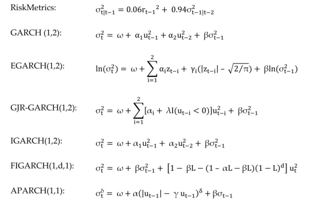
The models considered in this study include RiskMetrics EWMA, GARCH, EGARCH, GJR-GARCH, IGARCH, FIGARCH and APARCH. In the RiskMetrics model, = 0.94 is applied as in the model of J.P Morgan daily data (RiskMetricsTM – Technical Document 1986). For the GARCH genre models, the combination of p=1 and q=2 is applied for four following models: GARCH, EGARCH, GJR-GARCH and IGARCH as in the studies of Pagan and Schwert (1990), and Hansen and Lunde (2005) whereas FIGARCH and APARCH are estimated only for p=1 and q=1 because there are obstacles in the estimation process. The list of equations for studied models is presented in Table 1.
Table 1: The equations of studied volatility models
RiskMetrics: σ| = 0.06r+ 0.94σ| GARCH (1,2): σ= ω+ α u + αu + βσ EGARCH(1,2): lnσ = ω+ ! α "z"+ γ"|z"| – 72⁄ π "# + βlnσ GJR-GARCH(1,2): σ= ω+ ![α "+ λIu" < 0]u" "# + βσ IGARCH(1,2): σ= ω+α u + αu + βσ FIGARCH(1,d,1): σ= ω+ βσ + -1 − βL − 1 – αL −βL1 − LE1 u APARCH(1,1): σδ = ω+α|u | − γ uI+βσ
To achieve more robust conclusion about the forecasting performances between RiskMetrics and other GARCH genre models, SPA tests of Hansen (2005) are
conducted with six symmetric loss functions presented in chapter 3. In addition, MCS procedure (Hansen et al., 2010) is also conducted to find the set of the most appropriate model(s) in seven considered models. MULCOM package with available code to perform SPA tests provided by Hansen (2005) and code to do MCS procedure developed by Hansen et al (2011) is utilized to analyze empirical data for this study.
Back-testing VaR is also applied to validate the forecast performances of volatility models. The selected estimation and evaluation periods for each index are similar to the ones used in out-of-sample forecast evaluation procedure. VaR daily measures are computed with recursively updating estimate models every 20 days. Both 1% and 5%VaR for each index are calculated and examined with failure rate, Kupiec and dynamic quantile tests to evaluate the volatility forecast performances of studied models in real application.
6. EMPIRICAL RESULTS
6.1. Preliminary Data
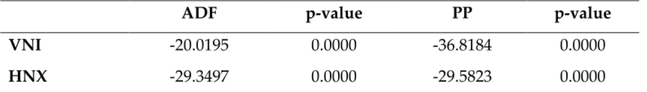
Initially the daily returns of the index are calculated as the first differences natural logarithms of the index daily price. Augmented Dickey-Fuller (ADF) and Phillips- Perron (PP) unit root tests are conducted to check the stationary of the return series. Table 2 presents these test results. The results indicate that the null hypothesis of a unit root can be rejected thoroughly at 1% significant level. Hence, both return series of the indices are stationary.
Table 2: Unit root tests
ADF p-value PP p-value
VNI -20.0195 0.0000 -36.8184 0.0000
HNX -29.3497 0.0000 -29.5823 0.0000
The table reports ADF and PP unit root tests without a time trend for the index return series. The lag length for the unit root tests is based on the Schwarz information criterion.
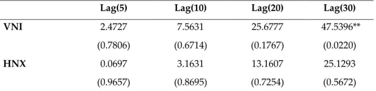
The appropriate orders for ARMA terms for the return series are selected based on both the Box-Jenkins method and Schwarz information criterion. The residual of the regression are the raw data used to estimate volatility and volatility models for further analysis. The Ljung-Box statistics in Table 3 show that the residual series have insignificant or slightly significant autocorrelations up to lag 30. It indicates that the selected models for both return series are quite appropriate.
Table 3: Ljung-Box test statistics
Lag(5) Lag(10) Lag(20) Lag(30)
VNI 2.4727 7.5631 25.6777 47.5396**
(0.7806) (0.6714) (0.1767) (0.0220)
HNX 0.0697 3.1631 13.1607 25.1293
(0.9657) (0.8695) (0.7254) (0.5672)
The table reports the Ljung-Box statistics at lag 5, 10, 20 and 30 of the residual series showing insignificant autocorrelations among the residuals. The figures in parentheses are the p-value. ** Significant at 5%
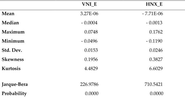
Table 4 presents descriptive statistics of the residual series. Both series are mildly skewed and the kurtosis of each series is higher than 3 indicating the leptokurtic nature. However, the kurtosis excess of HNX-index residual series (3.6029) is substantially higher than the one of VNI-index residual series (1.4829). Actually, according to the Jarque-Bera test results, the null hypothesis that the residual of each index returns has normal distribution is completely rejected. In most of the studied models, there is an assumption that the residual series has conditional normal distribution. The non-normal distribution of the index residual series can lead to substantial inaccuracy in volatility forecast performance.
Table 4: Descriptive statistics of the residual series
VNI_E HNX_E
Mean 3.27E-06 - 7.71E-06
Median - 0.0004 - 0.0013 Maximum 0.0748 0.1762 Minimum - 0.0496 - 0.1190 Std. Dev. 0.0153 0.0246 Skewness 0.1956 0.3827 Kurtosis 4.4829 6.6029 Jarque-Bera 226.9786 710.5421 Probability 0.0000 0.0000
Then the residual series are conducted ARCH Lagrange Multiplier tests with two lags. The following table - Table 5 - shows the results of the tests confirming that both residual series demonstrate significant ARCH effects.
Table 5: ARCH Lagrange Multiplier test statistics
VNI HNX
LM 352.7720 56.2975
p-value 0.0000 0.0000
The table reports the ARCH Lagrange Multiplier test results of the residual series showing the conditional variances of the return series demonstrate ARCH process.
After setting the residual series, the information set for each series is established based on the regression of M̂ against 12 lags. For VNI-index, the set of conditioning variables is ℱ® = ¯M̂ , M̂ , M̂G , M̂° , M̂± , M̂$ ² whereas for HNX-index, ℱG = ¯M̂ , M̂ , M̂ ² is selected. Then true volatilities of each series are estimated as the predictions from the regression of M̂ against the lags belonged to the conditioning variables set of each residual series ℱ©. The
descriptive statistics of the true volatility series estimated for the whole sample period are illustrated in Table 6.
Table 6: Descriptive statistics of proxied “true” volatility series
³´µ¶· ³ ¸µ¹ · Mean 0.000373 0.000808 Median 0.000305 0.000709 Maximum 0.001362 0.005191 Minimum 0.000234 0.000607 Std. Dev. 0.000167 0.000310 Skewness 1.853482 5.603330 Kurtosis 6.861032 58.184963
There are graphs illustrated proxied “true” variances and estimated variances series from seven studied models for each index are provided in the Appendix section.
6.2. Symmetric Forecast Error Measures
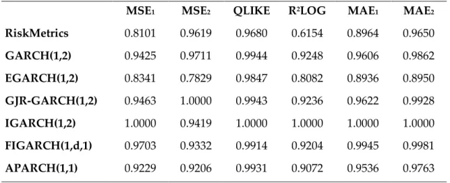
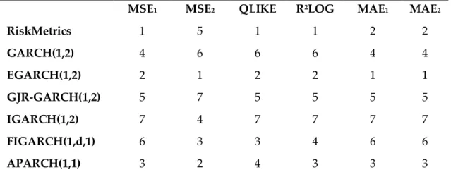
The relative forecast error statistics of seven models for two Vietnam stock indices are reported in Table 7 and the forecast performance evaluations in rank are presented in Table 8. For HNX index, EGARCH(1,2) model has the first ranks in all six loss measures while RiskMetrics has the last position in five out of six criteria except in MSE2. For VNI-index, EGARCH(1,2) is probably the model that has the best performance with three first-rank and three second-rank positions whereas IGARCH(1,2) performs worst in most of error measures except in MSE2. Moreover, RiskMetrics model has the first rank in three out of six forecast error statistics for VNI-index including MSE1, QLIKE and R2LOG.
Actually, the results showed in panel A of the following table corroborate the statement of Brailsford and Faff (1996) that the ranking of any forecasting model varies depending upon the choice of error statistics. The ranks of models are not corresponding through all six loss functions.
The findings related to RiskMetrics performance for HNX-index contradict the initial expectation. Based on the results of McMillan and Kambouroudis (2009), RiskMetrics model is expected to outperform other models for both indices. Therefore, the null hypothesis that RiskMetrics EWMA model provides better volatility forecasts than other considered GARCH type models for HNX-index can be soundly rejected but for VNI-index the hypothesis cannot be rejected. These hypotheses are examined further by applying the SPA test of Hansen (2205) to reach more robust conclusion about the forecast performance of RiskMetrics model.
Table 7: Relative forecast error statistics
Panel A: Relative forecast error statistics for VNI-index
MSE1 MSE2 QLIKE R2LOG MAE1 MAE2
RiskMetrics 0.8101 0.9619 0.9680 0.6154 0.8964 0.9650 GARCH(1,2) 0.9425 0.9711 0.9944 0.9248 0.9606 0.9862 EGARCH(1,2) 0.8341 0.7829 0.9847 0.8082 0.8936 0.8950 GJR-GARCH(1,2) 0.9463 1.0000 0.9943 0.9236 0.9622 0.9928 IGARCH(1,2) 1.0000 0.9419 1.0000 1.0000 1.0000 1.0000 FIGARCH(1,d,1) 0.9703 0.9332 0.9914 0.9204 0.9945 0.9981 APARCH(1,1) 0.9229 0.9206 0.9931 0.9072 0.9536 0.9763
Panel B: Relative forecast error statistics for HNX-index
MSE1 MSE2 QLIKE R2LOG MAE1 MAE2
RiskMetrics 1.0000 0.9641 1.0000 1.0000 1.0000 1.0000 GARCH(1,2) 0.9439 1.0000 0.9965 0.9629 0.9516 0.9689 EGARCH(1,2) 0.7660 0.7899 0.9712 0.7557 0.8455 0.8600 GJR-GARCH(1,2) 0.9393 0.9979 0.9967 0.9601 0.9431 0.9603 IGARCH(1,2) 0.9005 0.8840 0.9915 0.9270 0.9332 0.9410 FIGARCH(1,d,1) 0.8843 0.8626 0.9900 0.9156 0.9230 0.9264 APARCH(1,1) 0.8805 0.8050 0.9911 0.9205 0.9205 0.9115
The table presents the relative forecast error statistics of seven studied models. The relative error measure is calculated as a ratio of the actual statistic relative to the measure of the worst performing model.
Table 8: Ranks of symmetric error statistics
Panel A: Ranks of symmetric error statistics for VNI-index
MSE1 MSE2 QLIKE R2LOG MAE1 MAE2
RiskMetrics 1 5 1 1 2 2 GARCH(1,2) 4 6 6 6 4 4 EGARCH(1,2) 2 1 2 2 1 1 GJR-GARCH(1,2) 5 7 5 5 5 5 IGARCH(1,2) 7 4 7 7 7 7 FIGARCH(1,d,1) 6 3 3 4 6 6 APARCH(1,1) 3 2 4 3 3 3
Panel B: Ranks of symmetric error statistics for HNX-index
MSE1 MSE2 QLIKE R2LOG MAE1 MAE2
RiskMetrics 7 5 7 7 7 7 GARCH(1,2) 6 7 5 6 6 6 EGARCH(1,2) 1 1 1 1 1 1 GJR-GARCH(1,2) 5 6 6 5 5 5 IGARCH(1,2) 4 4 4 4 4 4 FIGARCH(1,d,1) 3 3 2 2 3 3 APARCH(1,1) 2 2 3 3 2 2
The table reports the ranks of studied model in each forecast error statistics. The error measures are calculated by the symmetric loss functions mentioned in section 3.2.1. The model with the lowest error statistic value has the highest order.
The relative error statistics showed in Table 7 indicate that the differences in the magnitudes of these forecast error statistics between models are small especially with QLIKE and MAE2. In addition, White’s note (2000) about the possibility that the results are obtained by chance rather than inherent superior performance of the identified model is also taken into consideration. Therefore,
the SPA test is conducted to get more powerful findings. The results of the SPA tests are presented in the next part of this chapter – section 6.4.
6.3. Asymmetric Forecast Error Measures
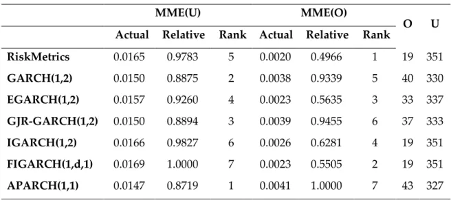
The same method of Brailsford and Faff (1996) is followed to calculate the mean mixed error as the asymmetric loss statistic. Table 9 shows the mean mixed error (MME) and number of times that each models over- and under-predict. The numbers of over- and under-predictions indicate that all models systematically under-predict. The systematic under-prediction is probably a result of selected sample period. This problem can cause difficulties in applying these models because under-prediction models cannot provide enough the worst expectation for the price risks. Indeed, this systematic under-prediction is also possibly caused by the inaccurate assumption about normal distribution of regression errors from a conditional mean model for returns while in reality they demonstrates leptokurtic feature. Therefore, the volatility models do not capture properly all the specifications.
The MME(U) statistics suggest the different results of forecast performances from the ones indicated by the symmetric loss statistics. For VNI-index, APARCH(1,1) model has the best performance while FIGARCH(1,d,1) performs worst with largest error measures. While for HNX-index, MME(U) favors the EGARCH(1,2) model while RiskMetrics ranks last. MME(U) prefers APARCH and EGARCH(1,2) models with high number of over-predictions become the best performance models compared to the worst RiskMetrics and FIGARCH(1,d,1). However, the MME(U) differences between models in magnitude are small as the symmetric forecast error differences. Hence, actually
the last rank models do not perform significantly worse than the first rank models.
On the other hand, because the MMU(O) statistic penalizes over-prediction errors more heavily, the differences in magnitude between models are larger. RiskMetrics models are ranked first for both indices with substantially small forecast errors compared to the others. APARCH(1,1) is ranked last for VNI-index while for HNX-VNI-index GARCH(1,2) has the worst performance. These results confirm once again the statements of Brailsford and Faff (1996) that the forecast evaluation results are highly sensitive to assessment criteria and the selected error statistic actually should be based on the ultimate purpose of forecasting procedure to choose an applicable model.
Table 9: Mean mixed error and numbers of under- and over-predictions
Panel A: MME and numbers of under- and over-predictions for VNI-index
MME(U) MME(O)
O U
Actual Relative Rank Actual Relative Rank
RiskMetrics 0.0165 0.9783 5 0.0020 0.4966 1 19 351 GARCH(1,2) 0.0150 0.8875 2 0.0038 0.9339 5 40 330 EGARCH(1,2) 0.0157 0.9260 4 0.0023 0.5635 3 33 337 GJR-GARCH(1,2) 0.0150 0.8894 3 0.0039 0.9455 6 37 333 IGARCH(1,2) 0.0166 0.9827 6 0.0026 0.6281 4 19 351 FIGARCH(1,d,1) 0.0169 1.0000 7 0.0023 0.5505 2 19 351 APARCH(1,1) 0.0147 0.8719 1 0.0041 1.0000 7 43 327
Panel B: MME and numbers of under- and over-predictions for HNX-index
MME(U) MME(O)
O U
Actual Relative Rank Actual Relative Rank
RiskMetrics 0.01793 1.0000 7 0.00052 0.2219 1 10 358 GARCH(1,2) 0.01570 0.8755 4 0.00232 1.0000 7 47 321 EGARCH(1,2) 0.01498 0.8353 1 0.00189 0.8125 3 46 322 GJR-GARCH(1,2) 0.01562 0.8709 2 0.00228 0.9795 6 44 324 IGARCH(1,2) 0.01567 0.8739 3 0.00216 0.9279 5 45 323 FIGARCH(1,d,1) 0.01576 0.8790 5 0.00189 0.8153 4 39 329 APARCH(1,1) 0.01599 0.8915 6 0.00158 0.6802 2 40 328
The table reports the MME(U) and MME(O) statistics calculated by equations in section 3.2.2 and the numbers of under- and over-prediction of each model. MME(U) is a mean mixed error which penalizes under-prediction more heavily while MME(O) is a mean mixed error which penalized over-prediction more heavily.
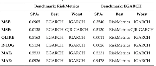
6.4. Superior Predictive Ability Test Results
The SPA tests of Hansen (2005) are conducted based on six symmetric loss functions mentioned in section 3.2.1 with 10000 bootstrap repetitions and ? = 0.5 as probability for stationary bootstrap. The results of model comparisons in the form of values are illustrated in Table 10 below. The p-value relates to the hypothesis that the benchmark model is the best model. The SPAc is asymptotically valid p-values controlled for the full set of models. The conclusion for the result of hypothesis testing based on the SPAc p-value.
Two benchmark models are considered in these SPA tests including RiskMetrics and EGARCH(1,2) to test the robustness of findings in section 6.2. Panel A shows the SPA test results for VNI-index, whereas Panel B contains the results for HNX-index. For HNX-index the p-values indicate that the RiskMetrics model is significantly outperformed by other models in terms of loss functions. However, for VNI-index, RiskMetrics is not outperformed by other models in most of loss functions with the exception of MSE2. Therefore, the studied hypothesis that RiskMetrics EWMA model provides better volatility forecasts than other considered GARCH type models for HNX-index is soundly rejected whereas the hypothesis for VNI-index is not rejected.
Moreover, for HNX index the SPA test results also suggest that EGARCH(1,2) model has best forecast performance as well as it is not outperformed by any other model in the considered group. On the other hand, for VNI-index, EGARCH(1,2) is outperformed by RiskMetrics in QLIKE and R2LOG. Thus for VNI-index, both RiskMetrics and EGARCH models can provide best forecast volatility. In addition, the best and worst models relative to the benchmark are