Christoph Hansknecht
Institute for Mathematical Optimization, Technical University Braunschweig, Germany [email protected]
Alexander Richter
Institute for Mathematical Optimization, Technical University Braunschweig, Germany [email protected]
Sebastian Stiller
Institute for Mathematical Optimization, Technical University Braunschweig, Germany [email protected]
Abstract
We develop a fast method to compute an optimal robust shortest path in large networks like road networks, a fundamental problem in traffic and logistics under uncertainty.
In the robust shortest path problem we are given an s-t-graph D(V, A) and for each arc a nominal lengthc(a) and a maximal increased(a) of its length. We consider all scenarios in which for the increased lengths c(a) + ¯d(a) we have ¯d(a)≤ d(a) and P
a∈A ¯ d(a)
d(a) ≤ Γ. Each path is
measured by the length in its worst-case scenario. A classic result [6] minimizes this path length by solving (|A|+ 1)-many shortest path problems. Easily, (|A|+ 1) can be replaced by|Θ|, where Θ is the set of all different valuesd(a) and 0. Still, the approach remains impractical for large graphs.
Using the monotonicity of a part of the objective we devise a Divide and Conquer method to evaluate significantly fewer values of Θ. This methods generalizes to binary linear robust problems. Specifically for shortest paths we derive a lower bound to speed-up the Divide and Conquer of Θ. The bound is based on carefully using previous shortest path computations. We combine the approach with non-preprocessing based acceleration techniques for Dijkstra adapted to the robust case.
In a computational study we document the value of different accelerations tried in the algo-rithm engineering process. We also give an approximation scheme for the robust shortest path problem which computes a (1 +)-approximate solution requiringO(log( ˆd/(1 +))) computations of the nominal problem where ˆd:= maxd(A)/min(d(A)\ {0}).
2012 ACM Subject Classification Mathematics of computing→Graph algorithms
Keywords and phrases Graph Algorithms, Shortest Paths, Robust Optimization
Digital Object Identifier 10.4230/OASIcs.ATMOS.2018.5
1
Introduction
We develop an algorithm for the cost-robust shortest path problem that significantly reduces the time needed to compute such paths on road networks in practice.
Finding a shortest path from a sourcesto a sinktin a graph with arc lengthsc(a) is a basic algorithmic problem with numerous applications, prominently involving navigation in road networks. Dijkstra’s algorithm is the backbone of most navigation applications, but it requires modern acceleration techniques to find within fractions of seconds a route in a network with several hundred thousands or millions of arcs, e.g., in the European road network.
© Christoph Hansknecht, Alexander Richter, and Sebastian Stiller; licensed under Creative Commons License CC-BY
18th Workshop on Algorithmic Approaches for Transportation Modelling, Optimization, and Systems (ATMOS 2018).
Unfortunately, input data in real-world applications is usually subject to changes, uncer-tainty or error. For travel times on roads, i.e., arc lengths in shortest path calculations, the change of data is often caused by varying traffic. Several approaches have been proposed to address this problem, including prediction of traffic, leading to time dependent travel times, as well as stochastic models. In this paper we study the classical cost-robust shortest path problem introduced by Bertsimas and Sim. Cost-robust optimization is an alternative approach to handle varying and uncertain data. It minimizes the cost a solution attains in its specific worst-case scenario out of a given set of scenarios. The advantage of the robust approach is that – within the limits of the scenario set – the objective is a deterministic, guaranteed upper bound on the actual travel time.
The scenario set for cost-robustness introduced by Bertsimas and Sim allows each cost coefficientc(a) of a linear cost function to deviate up to a – individual for each variablexa – maximal deviationd(a). In addition, the number of deviations in a scenario is limited by an input parameter Γ. This is equivalent to limiting by Γ the sum of the fractions of maximal deviations occurring in a scenario. Formally, for a given set of binary variables{xa, a∈A}
and vectorsc anddinN|A| the scenario set for the cost-functions is:
( c+ ¯d: 0≤d¯(a)≤d(a),∀a∈A∧X a∈A ¯ d(a) d(a) ≤Γ ) . (1)
For this scenario set the cost-robust counterpart of any binary linear program can be solved by solving at most (|A|+ 1)–many identical binary linear programs with different linear cost functions. More precisely, let Θ contain 0 and alld(a). Then one has to solve the problem for eachθ∈Θ and the cost function Γθ+P
Axa(c(a) + max(d(a)−θ,0)). Intuitively, the θenumerates over the smallest deviationd(a) occurring in the scenario. This highly cited result by Bertsimas and Sim applies to cost-robust shortest path, which can thus be found by solving one standard shortest path problem for each arc in the graph.
For a road network with several hundred thousand or millions of arcs this is impractical even when using fast shortest path algorithms. Therefore, we devise a method to significantly reduce the computational effort.
Starting from the Bertsimas and Sim result we use three ways towards practically useful cost-robust shortest path methods. First we reduce the number ofθ-values to be examined. Second, we use fast shortest path methods. Third, we reuse previous computations for bounds and goal-directed search, further accelerating the shortest path computations.
It has been proposed [21] that a cost-robust binary problem can be solved by Γ-many copies of the nominal problem. Unfortunately, this result contains a subtle error. We give a counter-example in the appendix which hints to our conviction that essentially|Θ|-many shortest path computations are needed in general.
Accelerated shortest path methods differ on whether they use preprocessing of the graph or not. In this paper, we restrict ourselves to not preprocess the graph. We instead use goal-directed and bidirectional search and adapt both to the cost-robust setting. The high deviations in the arc length in the robust case inhibit the use of traditional preprocessing techniques used for deterministic shortest paths.
1.1
Our contribution
We give an approximation scheme for general robust combinatorial optimization problems which can be used to compute a (1 +)-approximate solution using O(log( ˆd/(1 +))) computations of the original problem.
We introduce a Divide and Conquer approach together with lower bounds for general robust combinatorial optimization problems which can be used to reduce the number of computations of the original problem. The reduction of computations is achieved by carefully reducing the number of θ-values to be considered.
When applying this to the robust shortest path problem we additionally accelerate the computations of individual shortest paths using pruning and a goal-directed search tailored to the robust shortest path problem.
We give an efficient method to obtain lower bounds for the length of shortest paths with respect to cθ. We use these bounds to speed up the Divide and Conquer approach. We conduct a computational study showing the effectiveness of our techniques.
1.2
Organization of this paper
We begin by formally introducing the robust shortest path problem in Section 2. We restate the main theorem by Bertsimas and Sim and devise an approximation scheme for the robust shortest path problem. In Section 3 we propose a general framework designed to reduce the number of computations of shortest path computations required to solve a robust shortest path problem. The framework relies on Theorem 3 which is based on the fact that the costs of arcs are non-increasing with respect toθ. We augment this framework by applying shortest path acceleration techniques to the robust shortest path problem. These techniques are search pruning (see Section 4) and goal-direction (see Section 5). The Divide and Conquer framework relies on lower bounds in order to remove dominated values. In Section 6 we devise a method to derive lower bounds of high quality based on information obtained from previous shortest path computations. We include these lower bounds into our Divide and Conquer approach. In order to show the effectiveness of our approach we conduct a computational experiment in Section 7.
1.3
Related work
Robust optimization evolved as a vivid research field during the past decade and shows a broad range of applications, for recent surveys we refer to [5] and [13]. The popularity of robust optimization is in part due to a large area of applications such as network design and routing problems. Network design problem in particular suffer from uncertainty with respect to demands and construction costs. These uncertainties can be treated by adding robustness to the underlying model [3, 20]. Robustness against demand uncertainty is also an important topic in problems such as vehicle routing [11] and lot sizing [22].
An important question with respect to robust optimization is whether or not tractability is preserved for the robust counterparts of polynomially solvable problems. Whether or not this is the case depends on properties of the nominal problem as well as on the employed robust model. For some choices of models, such as minmax regret models, nominally tractable problems become NP-hard (see for example [12]). In contrast, in [6] Bertsimas and Sim introduced a very general robust model which can be applied to many combinatorial optimization problems while preserving tractability.
The model of Bertsimas and Sim has gained wide acceptance and formed a basis for the study of robust combinatorial optimization problems, in particular regarding problems related to the robustness of shortest paths. Büsing considered the problem of robustness and robust recoverability in [8, 7]. In this setting, after a robust scenario has been realized it is still possible to perform some modifications of the previously chosen path in order to recover from the incurring robust costs. The authors of [19] considered the robust shortest path problem
with respect to robust costs corresponding to a product of two factors attained according to the model of Bertsimas and Sim. In [21], Poss considered combinatorial problems which can be solved with a dynamic programming approach. The author claimed that the robust counterparts of such problems can be solved with a dynamic program with a size increased by at most Γ. Unfortunately the proof contains a subtle error and the result does not hold. We give a counter-example in the appendix.
Since the ordinary shortest path problem has many real-world applications, considerable effort was put into an accelerated computation. Over the years, different preprocessing techniques such as arc flags [18] and contraction hierarchies [14] were introduced (see [4] for a summary). Preprocessing techniques require an initial offline phase which is used to augment the underlying problem in order to speed up queries in a subsequent online phase. The techniques perform very well in practice, decreasing query times by several orders of magnitude. It was shown in [1] that the query time with respect to preprocessing techniques decreases asymptotically for graphs with lowhighway dimension, a requirement generally satisfied for road networks. A related area of research considers large-scale networks which occur for example in social graphs. Such networks can comprise more than a billion vertices some of which having extremely large degrees. Conventional preprocessing techniques can’t be applied in this case. The authors of [9, 16] introduced an inexact preprocessing based on landmarks which is comparable to the approach in [15] for road networks. In contrast the authors of [2] considered a preprocessing technique which either answers the query correctly (in more than 99 % of the queries conducted in their experiments) and fails otherwise.
2
The robust shortest path problem
The robust shortest path problem is defined on a directed graphD= (V, A) withnvertices andmarcs. Each arca∈Ahas costsc(a)∈Nand deviationsd(a)∈N. A parameter Γ∈N
governs the conservatism in accordance with the model of Bertsimas and Sim. Specifically, consider a pathP given as a sequence of arcs. A worst-case scenario in the scenario set defined by (1) can be assumed to increase the costs on Γ of the arcs belonging toP to the upper boundd, yielding a total cost of
X a∈P c(a) + max S⊆P |S|≤Γ X a∈S d(a). (2)
The following theorem shows that the robust shortest path problem can be solved in polynomial time. This theorem and its proof will form the basis of this paper.
ITheorem 1 (Bertsimas and Sim in [6]). The robust shortest path problem can be solved using at mostm+ 1computations of nominal shortest paths.
Proof. We are attempting to find a path minimizing the cost given by (2). We first consider a fixed pathP and rewrite the inner optimization problem in terms of variables denoting membership in the setS:
max X a∈P x(a)·d(a) s.t. X a∈P x(a)≤Γ 0≤x(a)≤1 ∀a∈P (3)
This program has the following dual: min Γθ+X a∈P y(a) s.t. y(a) +θ≥d(a) ∀a∈P θ, y(a)≥0 ∀a∈P (4)
It is easy to see that y(a) can be fixed to max(d(a)−θ,0). As a result, minimizing (2) is equivalent to finding a pathP minimizing
min
θ∈R≥0
Γθ+X
a∈P
c(a) + max(d(a)−θ,0) (5)
The functionθ7→max(d(a)−θ,0) is piecewise linear with a break point atd(a). Therefore the function θ7→min P∈PΓθ+ X a∈P c(a) + max(d(a)−θ,0) (6)
has break points atd(a) for eacha∈A. It will therefore attain its minimum either at 0 or at somed(a). Thus, a robust shortest path can be found with at mostm+ 1 nominal shortest path computations according to the costs defined by the corresponding values of θ. J Even though the shortest path problem is easily solvable in practice, the overhead of solving
m+ 1 variants renders the robust counterpart intractable in practice. Observe that the number of shortest path computations required in total does not actually depend on the number of arcs but rather on the cardinality of the set
Θ :={0} ∪ {d(a)|a∈A}. (7)
This suggests an approximation scheme based on solving an instance with a lower number of deviations:
ITheorem 2. Let dˆ:= maxd(A)/min(d(A)\ {0}), >0. A (1 + )-approximate solution of the robust shortest path problem can be computed with O(log( ˆd/(1 +))) computations of the nominal shortest path problem.
Proof. Let ¯d:M 7→R≥0be the values ofdrounded up to the next power of (1 +): ¯
d(a) := (1 +)dlog1+(d(a))e ∀a∈A. (8)
There are onlyO(log( ˆd/(1 +))) different values forθwith respect to ¯d, which implies that we have to solve only that many instances of the original problem in order to obtain a robust optimum with respect to ¯d. LetP be a solution of the robust problem with respect to the deviationsd. LetS⊆P be the set of at most Γ entries causing the robust cost contribution toP with respect tod. In the worst case, everyd(a) increases by a factor of less than (1 +) from dtod. Thus, the robust cost contribution with respect todis again caused by the entries inS, increasing the cost ofP by less than (1 +). J IRemark.
1. The approximation guarantee is tight: Consider an instance of the robust shortest path problem given by a digraph consisting of two parallel arcs with pairs of costs and deviations of (/2,(1 +)k+/2) and (0,(1 +)k+1), a parameter ofk∈N>0and Γ = 1. The robust shortest path has a cost of+ (1 +)k, whereas a robust shortest path for the rounded
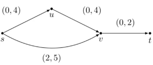
s u v t (0,4) (0,4) (2,5) (0,2)
Figure 1 An example for robust shortest paths not forming a tree. Pairs of numbers on arcs represent costs and deviations.
2. Bertsimas and Sim show that robust minimum cost network flow problems can be approximated to a factor of (1 +) in O(log(mθ/¯ )), where ¯θ := maxa∈Auada for
capacities u. However, robust network flows are not generally integral for integral capacities. Specifically, a robust network flow of one unit no longer corresponds to a path. 3. Recall that the shortest paths problem exhibits an optimal substructure: All shortest
paths leaving a common source vertexscan be chosen to form a tree in the underlying graph. This does no longer hold for robust shortest paths, as shown in Figure 1: For Γ = 2 the unique robust shortest path fromstotleads past vertexu, causing a cost of 8. The robust shortest (s, v) path consists solely of the lower arc.
3
Divide and Conquer
In this section we will describe the main idea used to reduce the number ofθ-values which have to be considered to compute a robust shortest path based on Theorem 1. We define
cθ(a) :=c(a) + max(d(a)−θ,0) and observe that this term is non-increasing inθ. The same holds for the cost of a pathP defined ascθ(P) :=Pa∈Pcθ(a). For a fixedθ we let
copt(θ) := min
P∈P(s,t)
cθ(P). (9)
Sincecopt(θ) is the minimum of non-increasing functions, it is non-increasing as well. In order to find a robust shortest path we will minimize the function
CΓ(θ) := Γθ+copt(θ). (10)
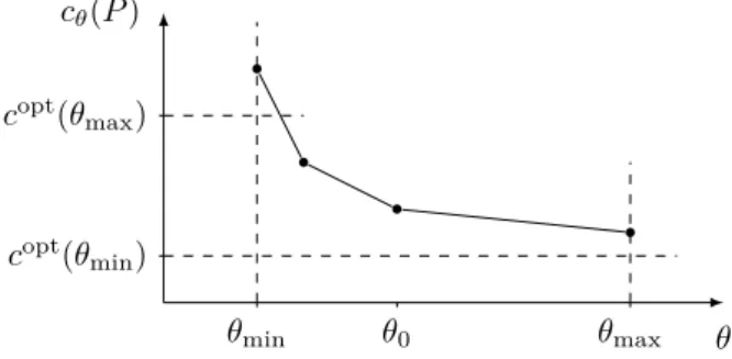
IfCΓ(θ) were a convex function in θ, we could use binary search or similar techniques in order to reduce the number of required shortest path computations. UnfortunatelyCΓ(θ) is not generally convex. We can however derive the following theorem from the fact that
copt(θ) is non-increasing:
ITheorem 3. Let θmin< θmax be in Θandθ∈Θ∩(θmin, θmax). 1. If copt(θmin) =copt(θmax), then it holds that CΓ(θ)≥CΓ(θmax). 2. Letθ∗ be in Θ. IfΓθ+copt(θmax)≥CΓ
θ∗, then the minimum overCΓ is not attained in
[θ, θmax).
Proof. For the first part note that since copt is non-increasing we have that copt(θ) =
copt(θmin) =copt(θmax). The result then follows from the definition ofCΓ. Turning to the second part, we letθ0 ∈[θ, θmax). We know thatCΓ(θ0)≥Γθ+copt(θmax)≥CΓ(θ∗) and thereforeCΓ(θ) is at least CΓ(θ∗).
J Both cases of Theorem 3 enable us to discard an interval of possible values forθ. We therefore use a Divide and Conquer approach as a general framework to speed up computations. The approach works as follows: We maintain a set of intervals of values in Θ together with
Algorithm 1:A Divide and Conquer algorithm for the robust shortest path problem.
AlgorithmDivideAndConquer
Input: DigraphD, costsc, deviationsd, parameter Γ, verticess, t
Output: A robust shortest (s, t)-path
S ← {Θ}
θ∗←The value of min(Θ), max(Θ) with lowerCΓ
whileS6=∅ do
Imin←The intervalIfromS with the lowest min(CΓ(min(I)), CΓ(max(I))) if Imincan be discarded then
continue
Imin←Remove dominated values fromImin
(Ilow, Ihigh)← Intervals such thatIlow∪Ihigh=Imin, |Ilow∩Ihigh|= 1, and ||Ilow| − |Ihigh|| ≤1
θmedian←The median value, single element inIlow∩Ihigh
θ∗←The value ofθ∗,θmedianwith lowerCΓ
S ←S∪ {Ilow, Ihigh}
returnThe path corresponding toθ∗
the currently best (w.r.t. CΓ) known value θ∗. We also ensure that the shortest paths with
respect to the minimum / maximum of each interval are computed before the interval is considered. At each step of the algorithm we select the interval which has the lowest value of
CΓat an endpoint. We first use Theorem 3 to try to discard the interval. If the interval can’t be discarded we proceed to remove any dominated values. We split the resulting interval into two halves which share exactly one value in Θ, compute the shortest path with respect to that value and decide whether or not to replaceθ∗. We then add the two intervals to the set and continue. The details are outlined in Algorithm 1.
Note also that Theorems 3 and 2 (and therefore also Algorithm 1) work for arbitrary robust combinatorial optimization problems.
4
Search pruning
Dijkstra’s algorithm explores a graph bylabeling andsettling vertices. A vertex is labeled when it is first explored. As soon as a shortest path connecting the vertex is known, the vertex is declared to be settled. Since we compute shortest (s, t)-paths for multiple cost functions cθ, we reuse information we have gathered from previous computations in order to
decrease the number of vertices which have to be labeled / settled in subsequent iterations of Dijkstra’s algorithm. The following theorem gives a sufficient condition for excluding vertices during searches:
ITheorem 4. Let v be a vertex and θ < θ0 whereθ, θ0∈Θ. LetPθ, Pθ0 be(s, v)-paths that are optimal with respect tocθ respectivelycθ0. Let
Γθ+cθ(Pθ)>Γθ0+cθ0(Pθ0). (11)
Then a robust shortest(s, t)-path is either attained for a value6=θor it does not contain v.
We can make the most of this theorem when we evaluate the values ofθ in a decreasing fashion. During these computations we maintain a map ¯C:V →R≥0. Think of ¯C(v) as a
known upper bound on the cost of a robust (s, v)-path which we initialize to ¯C≡ ∞. When we settle a vertexu6=tduring the search for a shortest path with respect tocθwe investigate each outgoing arc (u, v)∈A. The path leading tou together with (u, v) forms a pathP
leading tov yielding a value Γθ+cθ(P). If Γθ+cθ(P)>C¯(v) we do not have to label v. Otherwise we labelv and decrease ¯C(v) to Γθ+cθ(P).
5
Goal-direction
A common extension of Dijkstra’s algorithm is known as goal-directed search, introduced in [17]. It is based on a potentialπ:V →R≥0 such that the corresponding reduced costs
cπ(u, v) :=c(u, v)−π(u) +π(v) are non-negative for each (u, v)∈A. It is possible to derive a potential while searching for a shortest path. Consider a search fromtin the direction ofs. The resulting (partial) shortest-path treeT = (V(T), A(T)) is rooted attand contains all settled vertices. For eachv ∈V(T) we obtain a path P(v, t) leading fromv to the t. Let
cmax(T) be the maximum value ofc(P(v, t)) for v∈V(T). It is then easy to see that the following function is a potential:
π(v) := (
c(P(v, t)) forv∈V(T)
cmax(T) otherwise. (12)
In the robust setting, a potential with respect tocθ is also a potential forcθ0 withθ0 < θ (sincecθ0≥cθ). We use this observation in the following way: We first compute the potential (12) with respect toθmaxwhile finding the corresponding path using a backward search. In subsequent forward searches with respect to smaller values in Θ we use this potential. If the costs with respect toθ andθmax coincide, the arcs in the backward tree will have zero reduced cost. If all other arcs have nonzero reduced cost, then only the arcs in the shortest paths will have to be settled, greatly decreasing computation time. Intuitively, ifθ andθmax are close, then the potential computed fromθmaxis an excellent choice for the search with respect toθ.
6
Divide and Conquer for robust shortest paths
We refine Algorithm 1 by exploiting structural properties of the robust shortest path problem. We present our results for a unidirectional search here. In the appendix we show an extension to goal-directed and bidirectional searches in a more general setting.
Consider some intervalI:= [θmin, θmax] which appears in the course of Algorithm 1. As an invariant we have completed the Dijkstra search forθmin. We want to reuse labeling information of this search to derive lower bounds onCθΓ
0 for someθ0∈I. If such a lower
bound exceeds the best known upper bound forC∗, we disregardθ0. In order to accelerate the computation of a robust shortest path, the computation of the lower bound forCθΓ0 must be significantly faster than a computation of the path forcθ0.
We argue about a hypothetical (s, t)-pathPand its costcθ(P). The cost is non-increasing
and piecewise linear as a function inθ. It has breakpoints wheneverθ increases beyondd(a) for somea ∈P. From this point on the costca(θ) stays constant at c(a). We know the
valuescopt(θmin) andcopt(θ0) for some valuesθ0 ≥θmax. Whatever the value of cθ0(P), the cost ofP cannot decrease below these amounts when evaluated at the respective values (see Figure 2).
cθ(P) θ θmax θmin θ0 copt(θmax) copt(θmin)
Figure 2The costcθ(P) of someP. The cost atθ0has to be consistent withcopt(θmin),copt(θmax).
We go on to formulate a mixed integer program (shown in (13)) to choose an arc set minimizingcθ0. To make the formulation as strong as possible we choose the smallest possible set of arcs to include into this program: Let M ⊂Abe the set of scanned arcs, i.e. arcs having a tail which has been settled throughout the search for the shortest (s, t)-path forθmin. Furthermore, letMθmin ⊆M be the restriction ofM toactivearcs i.e. arcs withd(a)> θmin. It turns out to be sufficient to consider the arcs inMθmin to obtain a lower bound oncθ0.
We introduce a binary variable xa for eacha∈Adenoting whether or notais contained inP. The variabley models a lower bound on the costcθmin(P) of P yielding (13b). The negative slope ofcθ(P) at the point θmin corresponds to the number of active arcs in P. In the worst case we have cθ(P) = y−P
a∈Mθminxa(min(d(a), θ)−θmin) by subtracting
from y the contribution of the active arcs. In this case the objective (13a) equalscθ0(P). However, not all active arcs fromMθmin can occur inP because for such a pathP the value ofcθ0(P) might violate our observations of shortest path lengths forcopt(θ0). Thus we must raise the variabley to havecθ0(P)≥copt(θ0). Using the expression forcθ(P) from above we obtain (13c) and altogether the following theorem:
ITheorem 5. Given an arc setM of scanned arcs during a completed unidirectional search forcθmin, then a lower bound Oθ0≤c
opt(θ
0)is given by
Oθ0= min y−
X
a∈Mθmin
xa·(min(d(a), θ0)−θmin) (13a)
s.t. y≥copt(θmin) (13b)
y−X
a∈Mθmin
xa·(min(d(a), θ0)−θmin)≥copt(θ0)
∀θ0> θ0 with knowncopt(θ0)
(13c)
y≥0, x∈ {0,1}Mθmin (13d)
The theorem can in fact be further generalized to the bidirectional, goal-directed case. The generalized Theorem 9 and its proof may be found in Appendix A.
The following theorem states that boundsOθ obtained for multipleθby Theorem 5 are nonincreasing inθ. This observation can reduce the number of necessary bound computations throughout our algorithm. A proof follows from the more general Theorem 10 in Appendix A.
ITheorem 6. For each θmin< θ0< θ1 we have copt(θmin)≥Oθ0 ≥Oθ1 ≥c
opt(θ0) for all θ0 that were considered in (13c) for bothOθ0 andOθ1.
It is too time-consuming to solve (13) in order to compute a single bound. We therefore consider a relaxation of the program which can be solved a lot faster while still providing sufficient bounds. Observe that the program has the structure of a multi-dimensional
knapsack problem once we fix some value ofy. We first relax the integrality ofxtowards
x∈[0,1]Mθmin and consider a single valueθ0 =θmax for (13c). What remains is a fractional
one-dimensional knapsack problem where arcs correspond to knapsack items:
max X a∈Mθmin xa(min(d(a), θ0)−θmin)−y s.t. copt(θmin)≤y X a∈Mθmin
xa(min(d(a), θmax)−θmin)≤y−copt(θmax)
x∈[0,1]Mθmin
(14)
Suppose we fixy=copt(θmin). The optimum of the relaxation can be obtained by selecting items greedily w.r.t. their gain, i.e. gain(a) := (min(d(a), θ0)−θmin)/(min(d(a), θmax)−θmin). This leaves exactly one split itemawith fractional value forxa. We argue that increasingy
further is not beneficial: An increase ofy by will increase the capacity of the knapsack by
and thereby lead to increasedxa in a greedy optimum. The objective function changes
by(gain(a)−1) which is nonpositive because gain(a)≤1 for all arcs. It is therefore never advisable to increasey and we only have to sort the arcs inMθmin w.r.t. their gain in order solve problem (14) and obtain a boundOθ0. Observe that
gain(a) =
(θ0−θmin)/(θmax−θmin) ifd(a)≥θmax
(θ0−θmin)/(d(a)−θmin) ifd(a)< θmax andd(a)≥θ0 (d(a)−θmin)/(d(a)−θmin) = 1 ifd(a)< θmax andd(a)< θ0
(15)
Thus the value gain(a) decreases as d(a) increases and it is sufficient to sort the arcs in
Mθmin once according to d(a) in order to computeOθ0 for eachθ0 ∈Θ∩(θmin, θmax). We
incorporate thisrelaxed knapsack bound (RKB)into the Divide and Conquer approach and apply the generalization of Theorem 5 to goal-directed and bidirectional search.
IRemark (Preprocessing). As mentioned above, preprocessing techniques for the ordinary shortest path problem have been extensively studied in the past. Specifically, successful attempts have been made [10] to adapt preprocessing techniques to problems with time-dependent cost functions. Therefore it seems obvious to investigate these techniques with respect to applicability to the robust shortest path problem.
Existing preprocessing techniques operating on problems with changing cost functions generally rely on the ability to provide reasonable bounds on the values attained by the cost functions in order to prune the search space efficiently. Unfortunately, the costs of arcs vary widely betweenc andc+din the robust shortest path problem, making it impossible to derive meaningful bounds. As a result we were not able to find preprocessing techniques leading to a significant decrease in query time.
7
Computational experiments
7.1
Experimental network
Due to the long history of experimental evaluations of shortest path algorithms, instances of road networks are ready at hand. However, these networks generally lack data necessary to determine deviation values. Furthermore, shortest path experimentation is conducted on continent-sized networks which are as of yet too large to allow for the computation of robust shortest paths.
We therefore chose to construct a road network ourselves. To this end, we considered a subnetwork of the German road network given by the region of Lower Saxony1. We performed the following preprocessing steps in order to obtain a network suitable for routing purposes: 1. We filtered the file to only include ways with highwaytags, excluding certain highway types such as tracks / service road etc. This process yielded 1.93M nodes and 0.36M ways.
2. We constructed a graph by replacing ways with sequences of arcs, adjusting for one-way restrictions. The resulting graph has 1.93M vertices and 2.17M arcs.
3. We removed directed and undirected chains from the graph. Chains occur frequently as they are used to model the curvature of roads. Therefore the resulting graph shrinks to 0.37M vertices and 0.50M arcs.
4. Since queries for robust paths in an insufficiently connected graph skew computational results we extracted the largest (in terms of the number of vertices) strongly connected component which has 0.15M vertices and 0.23M arcs.
We defined the values of c andd on the network as follows: The nominal length c is defined as the time needed to traverse a segment in accordance with the legal speed limit. To definedwe assumed that a certain number of segments is affected by situations such as traffic accidents or road works. If a segmentais affected, the traveling speed drops from the legal speed limit to a value of at most 10 km/h. The value dis chosen such that c+d
corresponds to the travel time according to a speed of at most 10 km/h (whered(a) = 0 if the speed limit ofais already at most 10 km/h). To avoid numerical problems we rounded bothc anddto the nearest second, resulting in|Θ|= 1,043 different deviation values2. We further assumed that at most Γ = 5 road segments suffer from additional congestion.
7.2
Experimental methodology
In order to judge the performance of a shortest path algorithm, the query time of the algorithm is compared to that of Dijkstra’s algorithm without any preprocessing applied. This approach raises the following issue: The time to answer a query for a shortest (s, t)-path using Dijkstra’s algorithm is highly dependent on the choice of the verticessandt: If the distance ofsandt w.r.t. cis small compared to the diameter ofD, then the search explores only a small part ofD and finishes quickly. If on the other handsandtare far apart, then almost the entire graph is explored before a path is found.
This issue can be addressed with the notion of a Dijkstra rank: A search from a fixed sourcesusing Dijkstra’s algorithm will settle the vertices inDin the order3s=v
1, v2, . . . , vk.
We define the Dijkstra rank ofvj with respect tos as the valuej. Note that the distance fromstovj is non-decreasing and the query time using Dijkstra’s algorithm is increasing in the Dijkstra rank. For a pair (s, t) of vertices we define the Dijkstra rank of (s, t) by the Dijkstra rank oftwith respect tos.
In order to evaluate the performance of different robust shortest path algorithms we recorded the query time for randomly chosen pairs of vertices with similar Dijkstra ranks. More specifically, we selected pairs of vertices with ranks in [l·n, u·n) wherelanduform intervals of size of 10 % of|V|.
1 The initial data was obtained from the OpenStreetMap project,
seehttps://www.openstreetmap.org.
2 The accompanying data may be found at 10.6084/m9.figshare.c.4193588. 3 We assume that ties are broken consistently.
For each interval we measured the average query time for a sample of 500 random pairs of vertices in order to reduce measurement errors. All query times were obtained using an implementation in theC++programming language compiled using the GNU C++ compiler with the optimizing option “-O2”. All measurements were taken on an Intel Core i7-965 processor clocked at 3.2 GHz. We implemented Dijkstra’s algorithm using binary heaps. Depending on the Dijkstra rank of a pair of vertices, the running time of a shortest path query ranges up to≈35 ms.
7.3
Results regarding search accelerations
As a first step we evaluated the previously introduced approaches to accelerate individual searches without using the Divide and Conquer approach. The results are depicted in Figure 3a. We remark the following:
1. In order to achieve the best results regarding the goal-directed search we occasionally recompute the potential from scratch. Specifically, we keep track of how many vertices are settled during the recomputation of the potential as well as how many vertices are settled during each subsequent goal-directed search. If the latter amount is within a fraction ofαof the former, we reuse the potential in the search to be carried out in the next iteration. Otherwise, we mark the potential to be recomputed during the next query. We found experimentally that a factor ofα= 0.15 yields the best results.
2. Regarding the bidirectional goal-directed search: We found that the best choice for the combined potential is the average of the two potentials computed during the forward and backward search respectively. Additionally, we found that in order to obtain more accurate potentials it is worth the effort to compute the entire search tree fromstot in the forward search and vice versa in the backward search.
3. Both improvements over Dijkstra’s algorithm, the pruning and the goal-directed search, can be combined to speed up the computation even more.
Our findings show that while all approaches lead to reduced computation time, the goal-directed approaches works best, beating a plain evaluation using Dijkstra’s algorithm by almost an order of magnitude.
7.4
Results regarding the Divide and Conquer approach
We proceed to consider the impact of the Divide and Conquer approach on the query time (results are shown in Figure 3b). Combining Dijkstra’s algorithm with the generic Divide and Conquer approach (Algorithm 1) seems to have little effect on its own. Using the relaxed knapsack bound introduced in Subsection 6 however shows significant improvements. The combination of relaxed knapsack bounds and goal-direction yields the best results with a speedup factor ranging from 34 to 45 with an average of 38. A major contribution to this speed up is due to the fact that the Divide and Conquer approach cuts down on the required number of shortest path computations (see Figure 4): Dijkstra’s algorithm alone requires |Θ|-many shortest path computations regardless of the distance between source and target. The value is more than halved using the Divide and Conquer approach, it is cut down to less than ten percent if the relaxed knapsack bound is incorporated.
0.1 0.2 0.3 0.4 0.5 0.6 0.7 0.8 0.9 0 10 20 30 40 50
Dijkstra rank overn
A v erage query time ( s ) Dijkstra’s algorithm Dijkstra’s algorithm, pruning
Bidirectional, pruning Goal-directed Bidirectional, goal-directed
Goal-directed, pruning
(a)Average query time for different search acceler-ations. 0.1 0.2 0.3 0.4 0.5 0.6 0.7 0.8 0.9 0 10 20 30 40 50
Dijkstra rank overn
A v erage query time ( s )
Dijkstra’s algorithm, interval Goal-directed, interval Dijkstra’s algorithm, RKB
Bidirectional, RKB Goal-directed, RKB
(b)Average query time for selected combinations of search accelerations together with the Divide and Conquer approach.
Figure 3Average query time for different robust shortest path algorithms.
0.1 0.2 0.3 0.4 0.5 0.6 0.7 0.8 0.9
100 101 102 103
Dijkstra rank overn
A v erage n um b er of ev aluations
Dijsktra’s algorithm, interval Dijkstra’s algorithm, RKB Bidirectional, RKB
Figure 4Average number of shortest path computations for different variants of the Divide and Conquer approach. The naive algorithm consistently requires|Θ|= 1,043 evaluations.
8
Conclusion
We have presented an approximation scheme and a Divide and Conquer approach for general robust combinatorial optimization problems. The approximation scheme can be used to trade solution quality and running time. We introduced multiple techniques to accelerate the computation of robust shortest paths without abandoning solution quality ranging from the acceleration of individual queries to augmenting the Divide and Conquer approach by adding efficiently computable lower bounds of high quality. We evaluated our approaches by performing computational experiments on a digraph corresponding to a reasonable large road network. We found that a combination of the acceleration techniques decreased computation time by a factor of up to 45.
As the result for only Γ many shortest path computations does not hold and similar results seem unattainable in light of the counter-example, we give a currently best possible practical approach to solve the fundamental problem of shortest path in the classic Bertsimas Sim model for robustness.
References
1 Ittai Abraham, Amos Fiat, Andrew V. Goldberg, and Renato F. Werneck. Highway dimen-sion, shortest paths, and provably efficient algorithms. InProceedings of the Twenty-first Annual ACM-SIAM Symposium on Discrete Algorithms, SODA ’10, pages 782–793. Society for Industrial and Applied Mathematics, 2010.
2 Rachit Agarwal, Matthew Caesar, Brighten Godfrey, and Ben Y. Zhao. Shortest paths in less than a millisecond. CoRR, abs/1206.1134, 2012. doi:10.1145/2342549.2342559. 3 Alper Atamtürk and Muhong Zhang. Two-stage robust network flow and design under
demand uncertainty. Oper. Res., 55(4):662–673, 2007. doi:10.1287/opre.1070.0428. 4 Hannah Bast, Daniel Delling, Andrew Goldberg, Matthias Müller-Hannemann, Thomas
Pajor, Peter Sanders, Dorothea Wagner, and Renato F. Werneck. Route Planning in Transportation Networks, pages 19–80. Springer International Publishing, 2016. doi:
10.1007/978-3-319-49487-6_2.
5 Dimitris Bertsimas, David B. Brown, and Constantine Caramanis. Theory and applications of robust optimization. SIAM Review, 53(3):464–501, 2011. doi:10.1137/080734510. 6 Dimitris Bertsimas and Melvyn Sim. Robust discrete optimization and network flows.
Mathematical Programming, 98(1):49–71, 2003. doi:10.1007/s10107-003-0396-4. 7 Christina Büsing. The exact subgraph recoverable robust shortest path problem. In
Ravin-dra K. Ahuja, Rolf H. Möhring, and Christos Zaroliagis, editors,Robust and Online Large-Scale Optimization: Models and Techniques for Transportation Systems, pages 231–248. Springer Berlin Heidelberg, 2009. doi:10.1007/978-3-642-05465-5_9.
8 Christina Büsing. Recoverable robust shortest path problems. Networks, 59(1):181–189, 2012. doi:10.1002/net.20487.
9 Atish Das Sarma, Sreenivas Gollapudi, Marc Najork, and Rina Panigrahy. A sketch-based distance oracle for web-scale graphs. In Proceedings of the Third ACM Interna-tional Conference on Web Search and Data Mining, WSDM ’10, pages 401–410. ACM, 2010. doi:10.1145/1718487.1718537.
10 Daniel Delling and Dorothea Wagner. Time-dependent route planning. Robust and on-line large-scale optimization, 5868(1):207–230, 2009. doi:10.1007/978-3-319-17885-1_ 101392.
11 Maged M Dessouky, Fernando Ordonez, and Ilgaz Sungur. A robust optimization approach for the capacitated vehicle routing problem with demand uncertainty. IIE Transactions, 40(5):509–523, 2008. doi:10.1080/07408170701745378.
12 Maciej Drwal. Complexity of scheduling on parallel identical machines to minimize total flow time with interval data and minmax regret criterion. CoRR, abs/1412.4273, 2014. URL:http://arxiv.org/abs/1412.4273.
13 Virginie Gabrel, Cécile Murat, and Aurélie Thiele. Recent advances in robust optimization: An overview. European Journal of Operational Research, 235(3):471–483, 2014. doi:10. 1016/j.ejor.2013.09.036.
14 Robert Geisberger, Peter Sanders, Dominik Schultes, and Daniel Delling. Contraction hier-archies: Faster and simpler hierarchical routing in road networks. In Catherine C. McGeoch, editor, Experimental Algorithms: 7th International Workshop, WEA 2008 Provincetown, MA, USA, May 30-June 1, 2008 Proceedings, pages 319–333. Springer Berlin Heidelberg, 2008. doi:10.1007/978-3-540-68552-4_24.
15 Andrew V. Goldberg and Chris Harrelson. Computing the shortest path: A search meets graph theory. InProceedings of the Sixteenth Annual ACM-SIAM Symposium on Discrete Algorithms, SODA ’05, pages 156–165. Society for Industrial and Applied Mathematics, 2005.
16 Andrey Gubichev, Srikanta Bedathur, Stephan Seufert, and Gerhard Weikum. Fast and accurate estimation of shortest paths in large graphs. In Proceedings of the 19th ACM International Conference on Information and Knowledge Management, CIKM ’10, pages 499–508. ACM, 2010. doi:10.1145/1871437.1871503.
17 Peter E. Hart, Nils J. Nilsson, and Bertram Raphael. A formal basis for the heuristic deter-mination of minimum cost paths. IEEE Transactions on Systems Science and Cybernetics, SSC-4(2):100–107, 1968. doi:10.1109/tssc.1968.300136.
18 Moritz Hilger, Ekkehard Köhler, Rolf H. Möhring, and Heiko Schilling. Fast point-to-point shortest path computations with arc-flags. In The Shortest Path Problem, Proceedings of a DIMACS Workshop, Piscataway, New Jersey, USA, November 13-14, 2006, pages 41–72, 2006. doi:10.1090/dimacs/074/03.
19 Changhyun Kwon, Taehan Lee, and Paul Berglund. Robust shortest path problems with two uncertain multiplicative cost coefficients. Naval Research Logistics (NRL), 60(5):375– 394, 2013. doi:10.1002/nav.21540.
20 Supakom Mudchanatongsuk, Fernando Ordóñez, and Jie Liu. Robust solutions for network design under transportation cost and demand uncertainty. Journal of the Operational Research Society, 59(5):652–662, 2008. doi:10.1057/palgrave.jors.2602362.
21 Michael Poss. Robust combinatorial optimization with variable cost uncertainty. European Journal of Operational Research, 237:836–845, 2014. doi:10.1016/j.ejor.2014.02.060. 22 Muhong Zhang. Two-stage minimax regret robust uncapacitated lot-sizing problems with demand uncertainty. Operations Research Letters, 39(5):342–345, 2011. doi:10.1016/j. orl.2011.06.013.
A
Proofs
We begin by giving the proof of Theorem 4, which was stated as follows:
ITheorem 4. Let v be a vertex and θ < θ0 whereθ, θ0∈Θ. LetPθ, Pθ0 be(s, v)-paths that are optimal with respect tocθ respectivelycθ0. Let
Γθ+cθ(Pθ)>Γθ0+cθ0(Pθ0). (11)
Proof. Assume for a contradiction a shortest robust (s, t)-path P is attained forθandP
containsv. P consists of two subpaths, i.e. Pθ and a pathPv leading from vtot. We letP0
be the (s, t)-path which consists ofPθ0 andPv. We have:
CΓ(θ) = Γθ+cθ(Pθ) +cθ(Pv)
>Γθ0+cθ0(Pθ0) +cθ(Pv) ≥Γθ0+cθ0(Pθ0) +cθ0(Pv) ≥Γθ0+cθ0(P0)
(16)
We have used here thatcθ≥cθ0 which follows fromθ < θ0. This inequality implies thatP0 is a robust (s, t)-path which is shorter thanP which is clearly a contradiction. J We go on to present a more general variant of Theorem 5: We assume that we used a version of Dijkstra’s algorithm with respect to reduced costscπ
θmin obtained from a potential
πcomputed while conducting a search forcopt(θmin). During the execution of the search we settled vertices and obtained information regarding the shortest paths for the part of the graph we have explored: In a most general situation, this information is accessible via a fixed arc setM ⊆Aand various subsetsB⊆M together with boundsλ(B) fulfilling
λ(B)≤cπθmin(P∩M)∀P ∈ P(s, t) withB⊆P. (17)
We give some examples for this abstract setting, but first observe thatM should contain the arc set corresponding to some s−t cut to yield a bound λ(∅) > 0. Otherwise the right hand side of the inequality (17) is equal to 0 for some pathP withP∩M =∅. In case that a shortest path search completes, it determinescopt
π (t) as the length of a shortest
(s, t)-path forcπ
θmin, which leads toc
opt(θmin) =copt
π (t) +π(s)−π(t). This allows us to infer λ(∅) =copt(θmin)−π(s) +π(t) for the setM containing all scanned arcs. As before we let
Mθmin⊆M be the restriction to arcsawithd(a)> θmin.
IExample 7. If we stop unidirectional search prematurely we can use for M the set of arcs, that have a head with settled label andλ(∅) can be chosen as the last settled distance label from the search. This situation applies to Theorem 5. Additionally, for some arc
a= (u, v)∈Mθmin we can inferλ({a}) as the label thatv received fromuviaabecause it is a lower bound oncπθ
min(P∩M) for any (s, t)-pathP that containsa.
IExample 8. If some bidirectional Dijkstra search has been stopped prematurely, then let
Msbe the set of arcs that have their head settled by the search froms, and letMt contain the arcs with their tail settled by the search fromt. We can useM = Ms∪Mt and for λ(∅) the sum of both lastly settled distance labels in the searches fromsandt. For some
B={es, et}es∈Ms, et∈Mt,es6=et we get forλ(B) the sum of the head label fromes,
the tail label fromet, and both arc costscπθmin(es) +c
π
θmin(et). Similar bounds for singleton
B can be derived as well.
The idea of Theorem 9 is to compute a bound forcopt(θ
0) using the abstract bound information. In a suitable program we optimize over the arcs inMθmin that an imaginary pathP could contain to minimize cθ0(P). The program also makes use of values copt(θ0) known from
previous computations ifθ0 > θ.
ITheorem 9. Given a potentialπ, an arc set M, and a collection B ⊂2Mθmin, such that
thatπis also feasible forcθ0, we obtain a boundOθ0 ≤copt(θ0)whereOθ0 is an optimum of
min y−X
a∈Mθmin
xa(min(d(a), θ0)−θmin) (18a)
s.t. (λ(B) +π(s)−π(t))Y
b∈B
xb≤y ∀B∈ B (18b)
y−X
a∈Mθmin
xa(min(d(a), θ0)−θmin)≥copt(θ0)
∀θ0:θ0< θ0 withcopt(θ0)known (18c)
variables: y≥0, x∈ {0,1}Mθmin (18d)
Proof. LetP be any (s, t)-path. We show that cθ0(P)≥Oθ0 holds: Let us consider the arc setsP0,P¯ ⊆P given byP0 :=P∩M and ¯P :=P\P0.
We claim that settingxa:= 1 if and only ifa∈P0∩Mθmin together withy:=cθmin(P0) +
cθ0( ¯P) constitutes a feasible solution to (18) and the cost of this solution is then a lower
bound oncθ0(P). To get the lower bound we can first writecθ0(P0) in terms ofcθmin(P0):
cθ0(P0) =c(P0) +X a∈P0:d(a)>θ min max{d(a)−θ0,0}+cθmin(P 0)−cθ min(P 0) =c(P0) +X a∈P0:d(a)>θmin max{d(a)−θ0,0}+cθmin(P 0) − c(P0) + X a∈P0:d(a)>θ min max{d(a)−θmin,0} =cθmin(P 0) +X a∈P0:d(a)>θ min
(max{d(a)−θ0,0} −max{d(a)−θmin,0})
=cθmin(P0)−X a∈P0:d(a)>θ min (min(d(a), θ0)−θmin) =cθmin(P0)−X a∈Mθmin xa(min(d(a), θ0)−θmin) (19)
Here, the last equality holds, because by its definitionP0 is fully contained inM and all of its arcs withd(a)> θmin are contained inMθmin. With this expression we obtain
cθ0(P) =cθ0( ¯P) +cθ0(P0) =cθ0( ¯P) +cθmin(P0)−X a∈Mθmin xa(min(d(a), θ0)−θmin) =y−X a∈Mθmin xa(min(d(a), θ0)−θmin) ≥Oθ0 (20)
where the last inequality only holds if x, y is a feasible solution of (18). To prove this feasibility, we first consider (18b) and letB ∈ B. IfB*P∩Mθmin then the corresponding
Inequality (18b) has its left hand side equal to zero by the definition ofxand is feasible. So let B ⊆P ∩Mθmin which means that
Q
follows from the feasibility ofπ forcθ0, we first have: y=cθmin(P 0) +cθ 0( ¯P) =X a=(u,v)∈P0 (cπθmin(a) +π(u)−π(v)) +X a=(u,v)∈P¯ (cπθ0(a) +π(u)−π(v)) ≥X a=(u,v)∈P0 (cπθmin(a) +π(u)−π(v)) + X a=(u,v)∈P¯ (π(u)−π(v)) =cπθ min(P 0) +π(s)−π(t) (21)
Here the last equality follows from resolving the telescope sum for the (s, t)-pathP=P0∪P¯. Since B ⊆ P ∩M we can use the bound cπ
θmin(P
0) = cπ
θmin(P ∩M) ≥ λ(B) which now
implies (18b).
To show that Inequalities (18c) are satisfied, let θ0 ≥ θ0 and copt(θ0) be known. We know thatcopt(θ0)≤c
θ0(P) because P is an (s, t)-path. So we are interested in bounding
cθ0(P) =cθ0( ¯P) +cθ0(P0) against the left hand side of (18c). Becauseθ0 > θmin holds, we can do a similar calculation as before to expresscθ0(P0) in terms ofcθ
min(P 0): cθ0(P0) =cθ min(P 0)−X a∈Mθmin xa(min(d(a), θ0)−θmin) This implies copt(θ0)≤cθ0(P) =cθ0( ¯P) +cθ0(P0) =cθ0( ¯P) +cθ min(P 0)−X a∈Mθmin xa(min(d(a), θ0)−θmin) ≤cθ0( ¯P) +cθmin(P0)−X a∈Mθmin xa(min(d(a), θ0)−θmin) =y−X a∈Mθmin xa(min(d(a), θ0)−θmin) (22)
where the last inequality holds becauseθ0 > θ0impliescθ0( ¯P)≤cθ
0( ¯P). J
ITheorem 10. For eachθmin< θ0< θ1 such thatπis also feasible forcθ0 and cθ1 we have
copt(θmin)≥Oθ
0 ≥Oθ1 ≥c
opt(θ0)for all θ0 that were considered in (18c) for bothOθ
0 and
Oθ1.
Proof. We consider the definitions of (18) forθ0 andθ1 respectively. Observe that the sets
Mθmin, the bounds λ(B) as well as constraints (18b) and (18c) are independent ofθ0 and
thus both programs forOθ0 andOθ1 optimize over the same set of feasible solutions. The only difference is the objective function, where for somea∈Mθmin its coefficient forθ1is less
or equal than its coefficient forθ0. This impliesOθ0 ≥Oθ1 but alsocopt(θmin)≥Oθ
0: Note
thatOθmin is well-defined and contains only variabley becauseMθmin=∅. An optimum is
given by y=copt(θmin) and thus copt(θmin)≥Oθmin ≥Oθ0 because θ0 > θmin. Finally, it holds for someθ0 which was considered in (18b), that
Oθ1 =y− X a∈Mθmin xa(min(d(a), θ1)−θmin) ≥y−X a∈Mθmin xa(min(d(a), θ0)−θmin) ≥copt(θ0). J
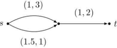
s t
(1,3)
(1.5,1)
(1,2)
Figure 5A counter-example to a claim regarding robust combinatorial optimization. Numbers on arcs represent costs and deviations.
B
A counter-example to a claim regarding robust combinatorial
optimization
We consider a claim made in [21] regarding a type of combinatorial optimization problems solvable by a dynamic programming (DP) algorithm. A combinatorial optimization problem is solvable by a DP algorithm if it can be expressed using a set of functional equations. More specifically, it is assumed that there is a set of states denoted byS with a subsetOof initial states and a final state N. The optimal cost of state s∈ S is given by F(s), the set of variables set to 1 in statesis denoted byq(s). The state p(s, i)∈Sis set to be the previous state ofswheresis obtained fromp(s, i) by fixing variablei∈q(s) to 1. The relationship between the states is assumed to be governed by the following set of functional equations:
(
F(s) = mini∈q(s){F(p(s, i)) +ci}, s∈S\ O
F(s) = 0, s∈ O (23)
In order to solve this problem the functional equation is applied to determine the optimal cost of new states until the optimal cost of the final state is determined. The question is whether the robust counterpart of such a problem can be solved in a similar manner using functional equations.
ITheorem 11(Theorem 6 in the original article). Consider an instance of a combinatorial optimization problem which can be solved inO(τ)for someτ:N→N by using the functional equations(23). Then, its robust version can be solved inO(Γτ)using the following functional equations:
F(s, α) = mini∈q(s){max(F(p(s, i), α) +ci, F(p(s, i), α−1) +ci+di)}, s∈S\ O,1≤α≤Γ
F(s,0) = mini∈q(s){F(p(s, i),0) +ci}, s∈S\ O
F(s, α) = 0, 0≤α≤Γ, s∈ O
(24)
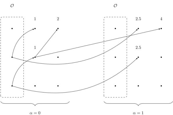
As an example of such a problem the authors consider the shortest path in a directed graph with conservative arc costs. It is well known that in this case the Bellman-Ford algorithm finds a shortest path by solving a dynamic program. As a counter-example to the claim stated above, we consider the graph in Figure 5 together with a parameter of Γ = 1. It should be apparent, that the robust shortest path in this case is the lower path with a total cost of 4.5. In order to compute the shortest path we start evaluating the functional equations for α= 0. In this the coefficients coincide with those of the original problem. The graph corresponding to these functional equations is shown in Figure 6. Unfortunately, the path resulting from applying the functional equations is the upper path which has total costs of 5. The failure is due to the fact that the equations do not take into account that the first arc on the upper path has a high value ofd.
O O α= 0 α= 1 1 1 2 2.5 2.5 4
Figure 6A depiction of the functional equations applied to the robust shortest path problem in Figure 5.
C
Figures and tables
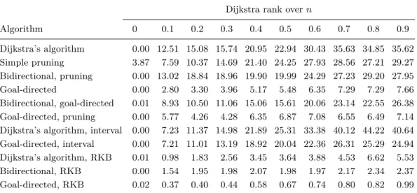
The following table contains the average query time plotted in Figures 3a and 3b. Regarding the distribution of the values: As is usually the case when it comes to the evaluation of running times, there is a certain variance in the recorded data. Figure 7 shows the distribution of running times for vertices with large Dijkstra ranks. Note that while the minimum / maximum query times are spread far apart, many of the individual values fall into much smaller intervals around the average. This behavior is consistent throughout the data and justifies the comparison based on the average query time.
Table 1Average query time in seconds for various algorithms with respect to different ranks
Dijkstra rank overn
Algorithm 0 0.1 0.2 0.3 0.4 0.5 0.6 0.7 0.8 0.9 Dijkstra’s algorithm 0.00 12.51 15.08 15.74 20.95 22.94 30.43 35.63 34.85 35.62 Simple pruning 3.87 7.59 10.37 14.69 21.40 24.25 27.93 28.56 27.21 29.27 Bidirectional, pruning 0.00 13.02 18.84 18.96 19.90 19.99 24.29 27.23 29.20 27.95 Goal-directed 0.00 2.80 3.30 3.96 5.17 5.48 6.35 7.29 7.29 7.66 Bidirectional, goal-directed 0.01 8.93 10.50 11.06 15.06 15.61 20.06 23.14 22.55 26.38 Goal-directed, pruning 0.00 5.77 4.26 4.28 6.35 6.87 7.08 6.55 6.49 7.14 Dijkstra’s algorithm, interval 0.00 7.23 11.37 14.98 21.89 25.31 33.38 40.12 44.22 40.64 Goal-directed, interval 0.00 7.21 11.01 13.19 18.92 20.04 22.36 26.31 25.29 24.94 Dijkstra’s algorithm, RKB 0.01 0.98 1.83 2.56 3.45 3.64 3.88 4.53 6.62 5.53 Bidirectional, RKB 0.00 1.54 1.95 1.98 2.07 1.98 1.97 2.17 2.34 2.37 Goal-directed, RKB 0.02 0.37 0.40 0.44 0.58 0.67 0.74 0.80 0.82 0.99 10 20 30 40 50 60 70 80 Goal-directed, RKB Bidirectional, RKB Dijkstra’s algorithm, RKB Goal-directed, interval Dijkstra’s algorithm, interval Goal-directed, pruning Bidirectional, goal-directed Goal-directed Bidirectional, pruning Simple pruning Dijkstra’s algorithm Query time (s)
Figure 7Distribution of the recorded running times. The boxes show minimum, first quartile, average, third quartile, and maximum for a rank of 0.9·n.