Streams with Online Mixture of Probabilistic PCA
Anastasios Bellas, Charles Bouveyron, Marie Cottrell, J´
erˆ
ome Lacaille
To cite this version:
Anastasios Bellas, Charles Bouveyron, Marie Cottrell, J´
erˆ
ome Lacaille. Model-based Clustering
of High-dimensional Data Streams with Online Mixture of Probabilistic PCA. Advances in Data
Analysis and Classification, Springer Verlag, 2013, 7, pp.281-300.
<
hal-00759945
>
HAL Id: hal-00759945
https://hal.archives-ouvertes.fr/hal-00759945
Submitted on 3 Dec 2012
HAL
is a multi-disciplinary open access
archive for the deposit and dissemination of
sci-entific research documents, whether they are
pub-lished or not.
The documents may come from
teaching and research institutions in France or
abroad, or from public or private research centers.
L’archive ouverte pluridisciplinaire
HAL
, est
destin´
ee au d´
epˆ
ot et `
a la diffusion de documents
scientifiques de niveau recherche, publi´
es ou non,
´
emanant des ´
etablissements d’enseignement et de
recherche fran¸
cais ou ´
etrangers, des laboratoires
publics ou priv´
es.
(will be inserted by the editor)
Model-based Clustering of High-dimensional Data
Streams with Online Mixture of Probabilistic PCA
Anastasios Bellas, Charles Bouveyron,Marie Cottrell and J´erˆome Lacaille
Received: date / Accepted: date
Abstract Model-based clustering is a popular tool which is renowned for its probabilistic foundations and its flexibility. However, model-based clustering techniques usually perform poorly when dealing with high-dimensional data streams, which are nowadays a frequent data type. To overcome this limita-tion of model-based clustering, we propose an online inference algorithm for the mixture of probabilistic PCA model. The proposed algorithm relies on an EM-based procedure and on a probabilistic and incremental version of PCA. Model selection is also considered in the online setting through parallel com-puting. Numerical experiments on simulated and real data demonstrate the effectiveness of our approach and compare it to state-of-the-art online EM-based algorithms.
Keywords model-based clustering · mixture of probabilistic PCA · data
streams·high-dimensional data·online inference
1 Introduction
Clustering is a data analysis tool which aims to group data into several ho-mogeneous groups. It usually occurs in applications in which a partition of the data is necessary. In particular, more and more scientific fields require to cluster data in order to understand or interpret the studied phenomenon.
Anastasios Bellas, Charles Bouveyron and Marie Cottrell
SAMM (EA 4543), Universit´e Paris 1
90, rue de Tolbiac, 75634 Paris Cedex 13, France E-mail: [email protected]
E-mail: charles.bouveyron,[email protected]
J´erˆome Lacaille
Snecma, Groupe Safran 77550 Moissy Cramayel, France E-mail: [email protected]
For instance, in the domain of aircraft engine health monitoring, Snecma, the french aircraft engine constructor, is interested in identifying a class sub-structure inherent to the data,i.e., a partition of the data, in order to better monitor an engine throughout its life,i.e.detecting malfunctions of the engine that can occur during a flight.
The clustering problem has been studied for years and can be split into two main families: heuristic and model-based techniques. Earliest approaches were based on heuristic or geometric procedures and relied on dissimilarity measures between the observations. The k-means algorithm [26] and the hi-erarchical clustering [16] are probably the most used heuristic procedures. Model-based clustering [18, 28] is also a popular approach which is renowned for its probabilistic foundations and its flexibility. One of the main advantages of this approach is the fact that the obtained partition can be interpreted from a statistical point of view.
However, modern data have some specificities which are challenging for most clustering methods and, in particular, for model-based clustering. In-deed, data are nowadays frequently high-dimensional, i.e. the number p of measured variables is large, and are also often available as data streams,i.e. the observations arrive over the time and the number of observationsn→ ∞. Such data, both high-dimensional and data streams, are more and more fre-quent in applications because of the recent technical advances in measure-ment devices. This is in particular the case in the applicative example that we consider in Section 4. Indeed, aircraft engines are nowadays made with sev-eral built-in high-frequency captors which produce large and high-dimensional data streams. The clustering of such data streams is in particular helpful for Snecma for the monitoring of their engines.
To overcome both issues, we propose to adapt a popular model-based clus-tering algorithm for high-dimensional data, called mixture of probabilistic principal component analyzers (MPPCA) [35], to the online setting. MPPCA is a clustering technique which models and clusters the data in low-dimensional subspaces. It allows to deal with high-dimensional data and has been applied with success to chemometrics [24] and hyperspectral image analysis [10] for instance. To make MPPCA able to cluster high-dimensional data streams, we develop hereafter an online EM-based algorithm which incorporates a proba-bilistic and incremental version of PCA. The resulting algorithm, called online MPPCA, is thus able to incrementally estimate mixture parameters while clus-tering the new observed data and keeping a low-dimensional representation of the whole data set. Let us notice that, even though we present here an online inference algorithm for the MPPCA model, it can be easily adapted for similar models such as MFA [20], PGMM [30] or HD-GMM [10, 11].
This article is organized as follows. Section 2 recalls the bases of model-based clustering and presents existing solutions for clustering high-dimensional data and data streams. Section 3 introduces the MPCCA model and presents its online inference algorithm. Model selection and data visualization in the online setting are also discussed in this section. Numerical experiments and
comparisons on simulated and real data are reported in Section 4. Finally, Section 5 gives some concluding remarks and directions for further work.
2 Related work
After having briefly reviewed the essentials of model-based clustering, this section presents existing solutions for clustering high-dimensional data and data streams.
2.1 Model-based clustering
Let us consider a data set ofnobservations {y1, . . . , yn} ∈Rp that one wants
to cluster into K homogeneous groups, i.e. determine for each observation
yi the value of its unobserved label zi such that zi = k if yi belongs to the
kth cluster. To do so, model-based clustering [18, 28] considers the overall population as a mixture of the groups and each component of this mixture is modeled through its conditional probability distribution. In this context, the observations{y1, . . . , yn} ∈Rpare assumed to be independent realizations of a
random vectorY ∈Rpwhereas the unobserved labels{z
1, ..., zn}are assumed
to be independent realizations of a random variableZ∈ {1, ..., K}. The set of pairs{(yi, zi)}ni=1 is usually referred to as the complete data set. By denoting
bypthe probabilistic density function of Y, the finite mixture model is:
p(y) =
K
X
k=1
πkfk(y), (1)
whereπk (such that PKk=1πk = 1) andfk respectively represent the mixture
proportion and the conditional density function of thekth mixture component. Furthermore, the clusters are often modeled by the same parametric density function. In this case, the finite mixture model is:
p(y) =
K
X
k=1
πkf(y|θk), (2)
whereθk is the parameter vector for thekth mixture component. Among the
possible probability distributions for the mixture components, the Gaussian distribution is certainly the one most frequently used for both theoretical and computational reasons. This specific mixture model is usually referred in the literature as the Gaussian mixture model (GMM).
Unfortunately, the inference of this model cannot be done in a straightfor-ward manner by maximizing the likelihood, since the group labels{z1, ..., zn}
algorithm iteratively maximizes the conditional expectation of the complete log-likelihood: E[ℓc(θ;y, z)|θ∗] = K X k=1 n X i=1 tiklog (πkφ(yi;θk)),
wheretik=E[z=k|yi, θ∗] andθ∗is a given set of mixture parameters. From
an initial solutionθ(0), the EM algorithm alternates two steps: the E-step and
the M-step. First, the expectation step (E-step) computes the expectation of the complete log-likelihoodE
ℓc(θ;y, z)|θ(q)
conditionally to the current value of the parameter set θ(q). Then, the maximization step (M-step)
max-imizesE
ℓc(θ;y, z)|θ(q)
overθ to provide an update for the parameter set. This algorithm therefore forms a sequence θ(q)
q which is guaranteed to
con-verge toward a local optimum of the likelihood [39]. For further details on the EM algorithm, the reader may refer to [27].
The two steps of the EM algorithm are iteratively applied until a stop-ping criterion is satisfied. The stopstop-ping criterion may be simply |ℓ(θ(q);y)−
ℓ(θ(q−1);y)|< εwhereεis a positive value to provide. It would be also possible
to use the Aitken’s acceleration criterion [25] which estimates the asymptotic maximum of the likelihood and allows to detect in advance the algorithm con-vergence. Once the EM algorithm has converged, the partition{zˆ1, . . . ,zˆK}of
the data can be deduced from the posterior probabilitiestik=P(Z =k|yi,θˆ)
by using themaximum a posteriori(MAP) rule which assigns the observation
yi to the group with the highest posterior probability.
2.2 Clustering of high-dimensional data
Model-based clustering methods unfortunately show a disappointing behavior in high-dimensional spaces which is mainly due to the fact that they are sig-nificantly over-parametrized. Since the dimension of observed data is usually higher than their intrinsic dimension, it is theoretically possible to reduce the dimension of the original space without loosing any information. For this rea-son, dimension reduction methods are frequently used in practice to reduce the dimension of the data before the clustering step. Feature extraction meth-ods, such as principal component analysis (PCA), or feature selection methods are very popular. However, dimension reduction techniques usually provide a sub-optimal data representation for the clustering step since they imply an information loss which could have been discriminative.
To avoid the drawbacks of dimension reduction, several recent approaches have been proposed to allow model-based methods to efficiently cluster high-dimensional data. Subspace clustering methods are searching to model the data in subspaces of much lower dimension and, thereby, avoid numerical problems and boost clustering capability. The Mixture of Factor Analyzers (MFA) may be considered as the earliest and the most general subspace clustering method. MFA both clusters the data and locally reduces the dimensionality of each
cluster. It extends the standard Factor Analysis (FA) model [6, 7], which links linearly the p-dimensional random vector Y to a d-dimensional latent vector
X:
Y =U X+µ+ǫ (3)
The p×d factor matrix U relates the two random vectors and µ ∈ Rp is a fixed location parameter. When d < p, X provides us with a parsimonious representation ofY. In this context,dis interpreted as the intrinsic dimension ofY.
The MFA model differs from the FA model in that it allows for different local factor models, in different regions of the input space, unlike FA which assumes a common factor model for the entire space. MFA is an extension of FA to a mixture of K factor analyzers. This approach , introduced by [20], was generalized a few years later by [29], which removed in particular the constraint on the variance of the noise. The MFA model was also extended by [5], which introduces the mixture of factor analyzers with common factor loadings (MFCA) by adding restrictions on the means and the covariance matrices.
A general framework for the MFA model was also proposed by [30] which includes the works of [20] and [29]. The authors propose a family of mod-els known as the expanded parsimonious Gaussian mixture model (EPGMM) family. They derive 12 EPGMM models by either constraining the terms of the covariance matrix to be equal or not, considering an isotropic variance for the noise term, or re-parametrizing the factor analysis covariance struc-ture. In a slightly different context, [10, 11] proposed a family of 28 parsimo-nious and flexible Gaussian models to deal with high-dimensional data. To do so, the authors re-parametrize the Gaussian mixture model into the group-specific eigenspaces and constrain model parameters within or across those eigenspaces. Let us note that both [30] and [10, 11] incorporates in their family the popular mixture of probabilistic principal component analyzers (MPPCA), initially proposed by [35].
Recently, [9] have proposed a family of mixture models which fit the data into a common discriminative subspace. The discriminative latent mixture (DLM) model, as it is called, differs from the FA-based models in the fact that the latent subspace is common to all groups and is assumed to be the most discriminative subspace of dimensiond. Moreover, the FA-based models choose the latent subspace(s) maximizing the projected variance whereas the DLM model chooses the latent subspace which maximizes the separation between the groups. Let us notice that the inference of the DLM models is not possible with the EM algorithm and [9] have proposed an alternative inference algorithm, called the Fisher-EM algorithm.
2.3 Clustering of data streams
In a probabilistic setting, incremental estimation approaches have naturally focused on extending the well-known EM procedure [14] for data stream clus-tering.
In [31], a view of EM that justifies incremental variants of the procedure is proposed. The authors define an objective functionF and reformulate the EM procedure as a two-step maximization ofF, with regard to the posterior class probability (E-step) and to the parameter vector (M-step). They show that their formulation is equivalent to standard EM. Moreover, they show that
F =P
iFi, where Fi is the value of F for thei-th observation,i = 1, . . . , n.
Based on the above decomposition, they derive a procedure which uses one observation at a time, maximizing its respective Fi. It can be shown that
the inferential import of the complete data can be summarized by a vector of sufficient statistics, which can be kept incrementally. The gain from such an incremental formulation is that it can speed up convergence, due to the parameter vector update taking place right after the update of the posterior class probability for each observation. In [37], the authors consider stochastic procedures for the recursive (online) update of the parameters of a statistical model using incomplete data. Their approach is general, but we will present here its application on EM. They give a recursive procedure to estimate the
Qfunction of the E-step of a standard EM. Based on this, they maximizeQ
with regard to the parameter vector in the M-step using the Newton-Raphson method. They also make use of the Fisher Information Matrix, which is the expectation of the Hessian Matrix. In this way, they finally derive a recursive (online) EM algorithm.
In [33], the authors based their work on [37] to develop an online CEM (for CEM, see [13]), which is a classification version of the standard EM. They reformulate CEM so that a stochastic version can be derived and they then adapt the update equations given by [37] for the M-step to the CEM context. Online EM was proposed in [12]. The authors make the hypothesis that the underlying statistical model of the data belongs to the exponential family. In their work, the standard EM procedure has been re-parametrized entirely into the space of sufficient statistics. They replace the standard E-step with a stochastic approximation step, which updates sufficient statistics by a convex combination of the old and the new ones. The combination is controlled by a sequence of decaying hyper-parameters γi, with 0≤γi ≤1 and i= 1, . . . , n,
wherenis the size of the dataset. Then, in the M-step, update formulas based on the sufficient statistics are being used to update the parameters.
There has also been an interest in developing approaches for incremental learning of Gaussian mixture models [3, 17, 22, 38] in the sense that new data are arriving over time and the GMM model must adapt itself appropriately. Unfortunately, these methods also suffer from the curse of dimensionality. The difference of these approaches to the online versions of EM mentioned above is that incremental GMM approaches are also concerned with controlling the
model complexity (number of mixture components, merging/splitting compo-nents, adding new ones etc.).
Finally, several works have also treated the problem of clustering data streams in a non probabilistic setting. In a number of these works [4, 15, 21, 32], some extensions of the popular k-means or k-median algorithms are developed in order to cluster data streams. A rather different approach is adopted in [1], where an online k-means-like clustering component is combined with an offline one, in order to better capture the evolution of the data stream. For a broad presentation of heuristic clustering algorithms for data streams, see [19].
Unfortunately, most of the above approaches suffer from the curse of di-mensionality and they cannot handle high-dimensional data.
3 Online mixture of PPCA
In this section, we restrict ourselves to the mixture of PPCA model and con-sider its online inference. Model selection and visualization of the data into low-dimensional subspaces are also discussed.
3.1 Mixture of probabilistic PCAs
The mixture of PPCA model [36] is a constrained version and probably the most popular extension of the MFA model. The MPPCA model assumes that the observed random vector Y ∈ Rp is, conditionally to Z, linked to a d -dimensional latent random vectorX ∈Rd through a linear transformation of the form:
Y|Z=k=UkX+µk+ǫ,
whereUk is thep×dorthogonal transformation matrix,µk∈Rp is the mean
vector of thekth factor analyzer andǫ∈Rp is a noise term. The dimensiond
of the latent vector is such thatd < pand assumed to be known (the choice of
dis discussed in Section 3.3). Moreover,ǫis assumed to be, conditionally toZ, a centered Gaussian noise term with a diagonal covariance matrixΨk=bkIp:
ǫ|Z=k ∼ N(0, bkIp).
Besides, the unobserved latent factorX ∈Rd is assumed to be, conditionally toZ, distributed according to a Gaussian density function such as:
X|Z=k ∼ N(0, Id).
This implies that the conditional distribution of Y is also Gaussian:
Y|X,Z=k∼ N(UkX+µk, bkIp), (4)
and its marginal distribution is therefore a mixture of Gaussians:
p(y) =
K
X
k=1
whereπkis the mixture proportion for thekth component,φis the multivariate
Gaussian density function andΣk =UktUk+bkIp.
In order to facilitate the description of our online inference procedure, let us slightly reparameterize the above model. Let us first introduce the orthonormal transformation matrixQk which is such that itsjth columnqkj =ukj/kukjk
whereukjis the corresponding column ofUk. If the transformation matrixQk
is orthonormal, it is then necessary to report the variance of the latent factor within the distribution of the latent factor. We therefore now assume that:
X|Z=k∼ N(0, ∆k),
where∆k = diag(λk1,. . ., λkd). The marginal distribution ofY is then still a
mixture of Gaussians but with covariance matricesΣk =Qtk∆kQk+bkIp. By
denoting by Wk = [Qk, Rk] the p×p matrix made of Qk and an
orthonor-mal complementary Rk, the projected covariance matrix WkΣkWkt has the
following form: WkΣkWkt= ak1 0 . .. 0 akd 0 0 bk 0 . .. 0 bk d (p−d)
where akj =λkj+bk andakj > bk , fork= 1, . . . , K and j = 1, ..., d. With
these notations, the mixture of PPCA model is fully parametrized by the set of parametersθ={πk, µk, Qk, akj, bk, d;k= 1, ..., K}.
It can be shown [10, 35] that, conversely to the MFA model, the MPPCA model is identifiable and its inference can be done using a simple EM algorithm. In particular, the update formula in the M step for the orientation matrices
Qk and the variance parametersakj andbk are as follows:
– the d columns of Qk are estimated by the eigenvectors associated with
thed largest eigenvalues of the empirical covariance matrixSk of the kth
group,
– akj is estimated by thejth largest eigenvalues ofSk,
– bk is estimated by: ˆ bk= 1 p−d tr(Sk)− d X j=1 ˆ akj .
These update formula allow in addition to see the strong link between MPPCA and the principal component analysis (PCA) method.
3.2 Online inference of mixture of PPCA
In order to extend MPPCA to the online setting, we develop hereafter an online EM-based algorithm which incorporates a probabilistic version of the incremental PCA [23]. We consider here an online setting where new observa-tions are arriving as time passes and each observation is being discarded after being processed.
Let us assume that we initially have observed a dataset ofn0 observations
(y1, ..., yn0) ∈R
p and that we have obtained an initial estimate ˆθ(n0) of the
parameter set from these observations. In practice, we obtain an initial esti-mation of the model parameters for every component k = 1, . . . , K with a standard MPPCA on this initial dataset. Let us setn=n0 and consider the
arrival of a new observationyn+1 ∈Rp. The objective is therefore to update
the estimate of θ from the only knowledge of ˆθ(n) and y
n+1. This will be a
two-step procedure which involves an E-step and a M-step.
3.2.1 The E-step
Before updating the estimate ofθ, it is necessary to compute the expectation of the complete log-likelihoodEhℓc(θ;y, z)|θˆ(n)
i
conditionally to the current estimate ˆθ(n). This quantity will be maximized in the second step to obtain the
new estimate ˆθ(n+1) ofθ. As for all mixture models, the computation of the
conditional expectation of the complete log-likelihood reduces, in the context of the MPPCA model, to the computation of the probabilitiest(kn+1)=P(Z=
k|Y =yn+1),k= 1, ..., K, that the new observation belongs to thekth mixture
component. These probabilities can be computed as follows:
t(kn+1)= πkφ yn+1; ˆθk(n) K P ℓ=1 πℓφ yn+1; ˆθ(ℓn) = 1 , K X ℓ=1 exp 1 2(Γ (n) k (yn+1)−Γ (n) ℓ (yn+1)) , (5) where the classification functionΓk has the following form:
Γk(y) =kµk−Pk(y)k2Ak+ 1 bk ky−Pk(y)k2+ d X j=1
log(akj)+(p−d) log(bk)−2 log(πk).
withkyk2
Ak =y
tA
ky,Ak =Qk∆k−1Qtk andPk(y) =QkQtk(y−µk) +µk.
3.2.2 The M-step
Once the posterior probabilities t(kn+1) have been computed, we update the model parameters such that they maximize E
ℓc(θ;y, z)|θ(n)
derive an online inference strategy which does not keep all past observations, it is necessary to make use of the following approximation:
Ehℓc(θ;y, z)|θ(n) i ≃Ehℓc(θ;y, z)|θ(n−1) i + K X k=1 t(kn+1)log (πkφ(xi;θk)).
Then, it is straightforward to show that the update formulas for the mixture proportionsπkand the component meansµk, for every componentk= 1, ..., K,
are: πk(n+1)=πk(n)+ 1 N+ 1 t(kn+1)−π(kn), (6) µ(kn+1)= 1 n(kn+1) n(kn)µk(n)−t(kn+1)yn+1 , (7) wheren(kn+1)=nk(n)+t(kn+1)andN = PK k=1 n(kn).
We then want to estimate the variance parameters Qk, akj and bk, for
k= 1, ..., K andj= 1, ..., d. We have seen, at the end of Section 3.1, that the maximization of E[ℓc(θ;y, z)|θ∗] with respect to these parameters is
equiv-alent to the eigen-decomposition of the empirical covariance matrixSk, and
this for each component k= 1, ..., K. The problem that we seek to solve can be therefore stated as follows: having already calculated eigenvectorsQ(kn)and eigenvalues Λ(kn) from the n first observations, we want to update those pa-rameters on the arrival of a (n+ 1)-th observation. In particular, on the arrival of the new observationyn+1, the new eigenproblem that we need to solve is:
Σk(n+1)Q(kn+1)=Q(kn+1)Λ(kn+1), (8) whereΛ(kn+1)= diag{λk1, ..., λkp} and this fork= 1, . . . , K.
To begin with, let us define:
gk(n+1)=Q(kn)Tt(kn+1)yn+1−µ(kn) , hk(n+1)=tk(n+1)yn+1−µ(kn) −Q(kn)gk,
where g(kn+1) is the projection of the observation on the subspace defined by the eigenvectors and h(kn+1) is the residue of the retro-projection on the original space. With these notations, the new eigenvectorsQ(kn+1) correspond to a rotation of the old ones plus the unit residue vector ˜hk:
˜ h(kn+1)= h(kn+1) h (n+1) k 2 ,if h (n+1) k 26= 0, 0, otherwise
and thus we have:
Q(kn+1)=hQ(kn),h˜k
i
R(kn+1) (9)
whereR(kn+1)is a rotation matrix of size (d+ 1)×(d+ 1). Note thatQ(kn)
is ap×dmatrix, since we have discarded thep−dless significant eigenvalues. The new covariance matrixΣk(n+1)for the classkis given by:
Σ(kn+1)= n (n) k n(kn+1)Σ (n) k + n(kn) n(kn+1)2 ¯ yy¯T (10)
where we have set ¯y = t(kn+1)yn+1 −µ(kn+1). Then, by substituting
Equa-tions 9 and 10 into Equation 8, we get:
h Q(kn),˜hk iT n(kn) n(kn+1) Σk(n)+ n (n) k n(kn+1) 2y¯y¯ T h Q(kn),˜hk i R(kn+1)=R(kn+1)Λ(kn+1)
The above problem can be written as:
n(kn) n(kn+1) Λ(kn) 0 0 0 + n (n) k n(kn+1)2 gkgTk γkgk γkgkT γ2k R (n+1) k =R (n+1) k Λ (n+1) k (11)
where we have setγk(n+1)= ˜hT
ky¯. The solution to this new eigenproblem yields
the rotation matrixR(kn+1)and the new eigenvaluesΛ(kn+1)directly. Then, the new eigenvectors can be obtained using Equation 9. Note that both Rk(n+1)
andΛ(kn+1) are square matrices of dimension (d+ 1), that is, we only need to solve an eigenproblem of dimension (d+ 1) and notp. The update formulas for the variance parametersakj andbk are then:
a(kjn+1)=Λ(kjn+1), b(kn+1)= 1 p−d tr(k)− d X j=1 Λ(kjn+1) ,
whereΛ(kjn+1)is thej-ith eigenvalue for the componentkand tr(k) =
p
P
j=1
Λ(kjn+1), fork= 1, . . . , Kand j= 1, . . . , d.
Algorithm 1The online MPPCA algorithm
1. Initialization: run a classical MPPCA on then0 first observations to provide an initial
set ˆθ(n0)of parameter estimates.
2. For each new observationyi:
– E-step: compute probabilitiest(ki), fork= 1, ..., K, using Equation (5),
– M-step: update parameter estimates using Equations (6-7) and solving the
incre-mental eigenproblem (11) allows to update ˆQk, ˆakj and ˆbk fork= 1, . . . , K and
j= 1, . . . , d.
3. Return after the last observationyN:
– set ˆθ(N)of model parameter estimates,
– data partition which can be deduce from the probabilities t(ki), i = 1, ..., N and
k= 1, ..., Kusing the MAP rule.
3.2.3 Algorithm and classification step
The online MPPCA algorithm that we proposed above is summarized in Al-gorithm 1. Even though the online MPPCA alAl-gorithm aims in the first place to infer the MPPCA model in the online setting, we are also interested in this work in obtaining a partition of the data after having processed the last ob-servation. To do so, it is necessary to add a classification step at the end of the online MPPCA algorithm to provide the expected clustering. In the model-based clustering framework, observations are usually assigned to a group using the maximum a posteriori (MAP) rule. The MAP rule assigns an observa-tion y ∈ Rp to the group for which it has the highest posterior probability
P(Z =k|Y =y) at the end of the algorithm. Therefore, this final classifica-tion step mainly consists in assigning the observaclassifica-tionyito the group with the
highestt(ki), fork= 1, ..., K andi= 1, ..., N.
3.3 Model selection in the online framework
The online MPPCA algorithm, as presented above, performs an almost au-tomatic inference of the MPPCA model, except for the hyper-parametersK
and d. Indeed, those parameters cannot be determined by maximizing the conditional expectation of the complete likelihood since they both control the model complexity. A popular and well-established way to determine the ap-propriate value for both K and d for the data at hand is to consider it as a model selection problem. Thus, the use of either the AIC [2], BIC [34] or ICL [8] criteria allows to find the appropriate values for K and d. However, since we consider in this work the online setting where past observations are not kept in memory, it is necessary to solve the model selection problem in an online manner as well. This is made possible nowadays by parallel computing. In our context, this consists in running in parallel several online MPPCA al-gorithms with different values for the hyper-parameters and select at the end the solution associated with the highest value for the model selection criterion.
3.4 Low-dimensional visualizations of the data
A final advantage of our online MPPCA algorithms is that is allows to pro-vide low-dimensional visualizations of the whole data set, even though the high-dimensional observations are not kept. The low-dimensional visualiza-tions consist in the projecvisualiza-tions of the data into theK estimated subspaces of the groups. If d is small compared to p, it is reasonable to keep in memory these low-dimensional representations of the data since the necessary memory size is γd =K×n×d instead of γp =n×p. However, this requires to be
able to update the low-dimensional projections into the group subspaces at the arrival of each new observation. At iterationn+ 1, this can be done after the M-step as follows:
xi(n+1)=xi(n)R(kn+1),
where R(kn+1) are the eigenvectors of the eigenproblem (11) and this for k= 1, ..., K andi= 1, ..., n.
4 Experiments
In this section, we present and discuss the results of the experiments that we performed on simulated and real data, with the aim of validating the perfor-mance of online MPPCA and of comparing it to other online algorithms.
4.1 An introductory example
We begin by an introductory experiment on simulated data. We have generated a dataset ofn= 12000 observations (y1, . . . , yn)∈Rpbased on the assumption
that data live in low-dimensional subspaces, withp= 30 andK= 3. Hereafter, we refer to this dataset asX30. The mixture proportions areπ1= 0.4 andπ2=
π3= 0.3. For simplicity, we have considered that for each class, the variance
is common across all dimensions, that isakj =ak, fork= 1, . . . , K andj =
1, . . . , d. We have seta1= 150,a2= 75,a3= 50,b1=b2=b3= 5 andµ1=0,
µ2={0, . . . ,5, . . . ,0} andµ3={0, . . . ,−5, . . . ,0}, withµ1, µ2, µ3 ∈ Rp. We
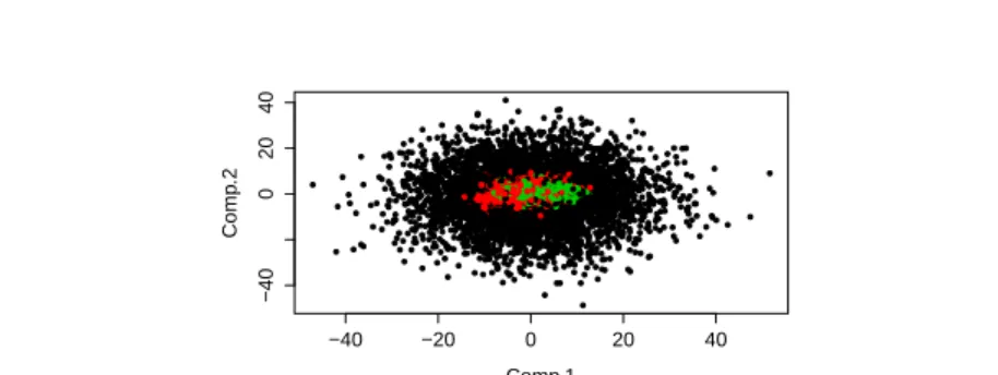
have set the intrinsic dimension (dimension of the subspaces) atd= 2. Figure 1 shows the projection of the simulated dataset ofp= 30 on the PCA axis. We can see that it is a challenging dataset for a clustering algorithm.
Note that we have initialized online MPPCA with n0= 100 observations.
The algorithm was given the true values forKandd. In practice, one has run it with different values ofKanddand keep the values giving the best model (according to a criterion,i.e.BIC [34]).
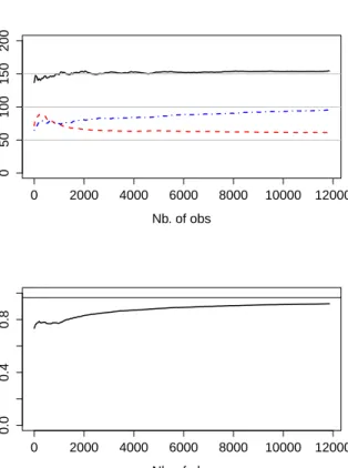
Figures 2 show the results obtained by online MPPCA for the datasetX30.
The upper part of the Figure shows the evolution of the estimation of MPPCA parametersakfork= 1, . . . , Kversus the number of the observations.
−40 −20 0 20 40 −40 0 20 40 Comp.1 Comp .2
Fig. 1 Simulated data fromK = 3 classes (represented by the three colors) of original
dimensionp= 30, projected on the PCA axis. We can see that it is a challenging dataset
for a clustering algorithm.
that as the number of observations grows, online MPPCA converges towards the true value of the parameters.
The lower part of the Figure shows the evolution of clustering accuracy ver-sus the number of observations for online MPPCA. We can see that clustering accuracy given by online MPPCA constantly increases as new observations are arriving, converging to the accuracy given by a standard MPPCA model which passes over data multiple times.
4.2 Comparison with online EM and online CEM
In this second experiment, we compare online MPPCA to two other online algorithms, online EM [37] and online CEM [33]. Note that these algorithms to which we compare have not been designed to handle high-dimensional data. In this experiment, we have usedX30, the high-dimensional simulated dataset
presented above, as well as a second simulated dataset of lower dimension (p= 10), generated with the same parameters as the former. We will refer to this new dataset asX10. Our goal was to study the behaviour of the three
al-gorithms in low dimension and then illustrate the capability of online MPPCA to cluster efficiently even in high dimension.
We have evaluated the three algorithms on the quality of their estimation of the class means and on the accuracy of the clustering produced. The quality of the estimation of the means was taken to be the square of the distance of the estimated means to the true ones, averaged over allK= 3 classes
eµ= 1 K K X k=1 1 p p X j=1 (ˆµkj−µkj)2
Online MPPCA, online EM and online CEM were initialized 30 times by a standard MPPCA, an EM and a CEM, respectively, of which the initialization
0 2000 4000 6000 8000 10000 12000 0 50 100 150 200 Nb. of obs P ar ameters a_k 0 2000 4000 6000 8000 10000 12000 0.0 0.4 0.8 Nb. of obs Cluster ing accur acy
Fig. 2 (Top) Evolution of the estimated parametersak for the dataset X30 versus the number of observations for online MPPCA. Horizontal lines correspond to the true values
of the parameters. (Bottom) Clustering accuracy evolution for the datasetX30 versus the
number of observations for online MPPCA. The solid horizontal line corresponds to the clustering accuracy given by a standard MPPCA, which passes multiple times over data.
giving the greatest BIC value was kept. Figure 3 and Figure 4 show the com-parative performance (error estimation measure eµ and clustering accuracy)
of online MPPCA (black), online EM (red) and online CEM (blue) for the datasetsX10andX30, respectively.
For the dataset X10 it is clear, both from the clustering accuracy and
the estimation error eµ that online MPPCA converges faster than the other
two algorithms. Online CEM converges faster than online EM, a result in compliance with conclusions made in [33].
For the dataset X30, we can see that online MPPCA clearly outperforms
the other two algorithms, even in high dimensionp= 30. As expected, high dimensionality affects the clustering performance of both online EM and online CEM. Note here that we have not compared the three algorithms in p >30 because online CEM in particular cannot handle such a dimensionality due to numerical problems.
0 2000 4000 6000 8000 10000 12000 0 1 2 3 4 5 6 7 Nb. of obs eµ 0 2000 4000 6000 8000 10000 12000 0.0 0.4 0.8 Nb. of obs Cluster ing accur acy
Fig. 3 (Top) Evolution of eµ for the datasetX10versus the number of observations for online MPPCA (black), online EM (red) and online CEM (blue). (Bottom) Clustering
ac-curacy evolution for the datasetX10versus the number of observations for online MPPCA
(black), online EM (red) and online CEM (blue).
4.3 Application to aircraft engine health monitoring
In the aircraft engine domain, the monitoring of engine health is a crucial task. Snecma, the french aircraft engine constructor, performs such tests in a test bench environment. A multitude of engine or bench parameters are measured, such as bench pressure, engine temperature, engine speed etc. Some of them are parameters of the environment of the test defined by external conditions and the manipulations performed by the test pilot (air pressure, rotation speed), while other are internal parameters of the engine (inside temperature and pressure etc.). The former are called exogenous, while the latter endogenous. We are typically interested in the endogenous variables.
Typically, there exists different phases during a flight, called flight modes: taking off, cruising, landing etc. Each test consists of a sequence of alternating stationary and non-stationary phases at different levels. The stationary phases correspond in general to such flight modes, while the non-stationary ones
re-0 2000 4000 6000 8000 10000 12000 0.0 1.0 2.0 3.0 Nb. of obs eµ 0 2000 4000 6000 8000 10000 12000 0.0 0.4 0.8 Nb. of obs Cluster ing accur acy
Fig. 4 (Top) Evolution of eµ for the datasetX30versus the number of observations for online MPPCA (black), online EM (red) and online CEM (blue). (Bottom) Clustering
ac-curacy evolution for the datasetX30versus the number of observations for online MPPCA
(black), online EM (red) and online CEM (blue).
flect the transition between two such phases. Nevertheless, a flight mode can include multiple stationary phases, that is, a stationarity control on the data is not enough to detect the flight modes.
Aircraft engineers can identify these modes by looking at the data but this can be extremely time-consuming. Moreover, due to the high dimensionality of data, there can be relations that humans cannot perceive. Note that by knowing, at any given time, in which flight mode the engine currently is, tasks like anomaly detection can be performed much more reliably, since the ’local’ context of the data (flight mode specificities) is also taken into account.
Here, we initially consider a streaming dataset ofn= 4683 observations and
p= 173 variables, issued from an engine bench test. Expert advice provided us with a configuration of 4 endogenous variables and 6 exogenous. Therefore, we consider only thosep= 10 variables out of 173. We then treat them in order to remove the influence of the exogenous variables to the endogenous ones. In
Subspace of cluster 1 Subspace of cluster 2 Subspace of cluster 3
Subspace of cluster 4 Subspace of cluster 5 Subspace of cluster 6
Subspace of cluster 7 Subspace of cluster 8 Subspace of cluster 9
Subspace of cluster 10 Subspace of cluster 11 Subspace of cluster 12
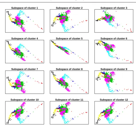
Fig. 5 Projection of aircraft engine data on each of the class-specific subspaces of dimension
d= 2. Colors correspond to different classes according to the clustering produced by online
MPPCA. The projections give an interesting insight into the classes.
the end, we have a dataset ofp= 4 endogenous variables, clean of exogenous influence.
We use this dataset to illustrate that online MPPCA can facilitate the detection of homogeneous groups of aircraft engine data. Such a group can coincide with a flight mode, subsume multiple flight modes or correspond to a part of a flight mode. Expert analysis is then needed to analyse these groups and relate them to the engine or to actual events (if any) that occured during a test sequence.
We launched online MPPCA with K = 12 and d = 2. In fact, we tested different combinations of the values of these two parameters and we kept the one giving the greatest BIC value. The initial dataset size was set atn0= 300.
Figure 5 shows the projection of the data onto each one of the class-specific subspaces given by online MPPCA, after having processed all the observations. Colors correspond to different classes according to the clustering produced by online MPPCA. We can see that the projections give an interesting insight into the clustering induced by online MPPCA. Clusterings in each subspace
can provide aircraft engineers with a much richer information on a possible inherent substructure of the data.
5 Conclusion
We have proposed an online inference algorithm for the MPPCA model which relies on an EM-based procedure and a probabilistic and incremental version of PCA. The proposed strategy allows to incrementally update, at the ar-rival of a new observation, the estimates of the MPPCA parameters. It allows also to provide low-dimensional visualizations of the data based on sufficient information. Model selection is also considered in the online setting through parallel computing. Numerical experiments on simulated and real data have shown that the online MPPCA algorithm performs better in high-dimensional spaces compared to existing online EM-based algorithms. Among the possible extensions for this work, it could be interesting to consider the re-computation of the posterior probabilities for all observations (including past observations) in the E-step based on the kept projected data.
References
1. Aggarwal, C., Han, J., Wang, J., Yu, P.: A framework for projected clustering of high dimensional data streams. In: Proceedings of the Thirtieth international conference on Very large data bases-Volume 30, pp. 852–863. VLDB Endowment (2004)
2. Akaike, H.: Likelihood of a model and information criteria. Journal of econometrics
16(1), 3–14 (1981)
3. Arandjelovi´c, O., Cipolla, R.: Incremental learning of temporally-coherent Gaussian
mixture models. (2006)
4. Babcock, B., Datar, M., Motwani, R., O’Callaghan, L.: Maintaining variance and
k-medians over data stream windows. In: Proceedings of the twenty-second ACM
SIGMOD-SIGACT-SIGART symposium on Principles of database systems, pp. 234– 243. ACM (2003)
5. Baek, J., McLachlan, G., Flack, L.: Mixtures of factor analyzers with common factor loadings: Applications to the clustering and visualization of high-dimensional data.
Pat-tern Analysis and Machine Intelligence, IEEE Transactions on32(7), 1298–1309 (2010)
6. Bartholomew, D., Knott, M., Moustaki, I.: Latent variable models and factor analysis: a unified approach, vol. 899. Wiley (2011)
7. Basilevsky, A.: Statistical factor analysis and related methods: theory and applications, vol. 418. Wiley-Interscience (2009)
8. Biernacki, C., Celeux, G., Govaert, G.: Assessing a mixture model for clustering with the integrated completed likelihood. Pattern Analysis and Machine Intelligence, IEEE
Transactions on22(7), 719–725 (2000)
9. Bouveyron, C., Brunet, C.: Simultaneous model-based clustering and visualization in
the fisher discriminative subspace. Statistics and Computing22(1), 301–324 (2012)
10. Bouveyron, C., Girard, S., Schmid, C.: High-dimensional data clustering.
Computa-tional Statistics & Data Analysis52(1), 502–519 (2007)
11. Bouveyron, C., Girard, S., Schmid, C.: High-dimensional discriminant analysis.
Com-munications in Statistics—Theory and Methods36(14), 2607–2623 (2007)
12. Capp´e, O., Moulines, E.: Online EM algorithm for latent data models. Journal of
the Royal Statistics Society: Series B (Statistical Methodology)71, 1–21 (2009). URL
13. Celeux, G., Govaert, G.: A classification em algorithm for clustering and two stochastic
versions. Computational statistics & Data analysis14(3), 315–332 (1992)
14. Dempster, A., Laird, N., Rubin, D., Others: Maximum likelihood from incomplete data via the EM algorithm. Journal of the Royal Statistical Society. Series B (Methodological)
39(1), 1–38 (1977). DOI http://dx.doi.org/10.2307/2984875
15. Domingos, P., Hulten, G.: A general method for scaling up machine learning algorithms
and its application to clustering. In: MACHINE LEARNING-INTERNATIONAL
WORKSHOP THEN CONFERENCE-, pp. 106–113 (2001)
16. Duda, R., Hart, P., Stork, D.: Pattern classification and scene analysis 2nd ed. (1995) 17. Figueiredo, M., Jain, A.: Unsupervised learning of finite mixture models. Pattern
Anal-ysis and Machine Intelligence, IEEE Transactions on24(3), 381–396 (2002)
18. Fraley, C., Raftery, A.: Model-based clustering, discriminant analysis, and density
esti-mation. Journal of the American Statistical Association97(458), 611–631 (2002)
19. Gaber, M., Zaslavsky, A., Krishnaswamy, S.: Mining data streams: a review. ACM
Sigmod Record34(2), 18–26 (2005)
20. Ghahramani, Z., Hinton, G., et al.: The em algorithm for mixtures of factor analyzers. Tech. rep., Technical Report CRG-TR-96-1, University of Toronto (1996)
21. Guha, S., Mishra, N., Motwani, R., O’Callaghan, L.: Clustering data streams. In: Foun-dations of computer science, 2000. proceedings. 41st annual symposium on, pp. 359–366. IEEE (2000)
22. Hall, P., Hicks, Y., Robinson, T.: A method to add gaussian mixture models (2005) 23. Hall, P., Marshall, D., Martin, R.: Incremental eigenanalysis for classification. In: British
Machine Vision Conference, vol. 1, pp. 286–295. Citeseer (1998)
24. Jacques, J., Bouveyron, C., Girard, S., Devos, O., Duponchel, L., Ruckebusch, C.: Gaus-sian mixture models for the classification of high-dimensional vibrational spectroscopy
data. Journal of Chemometrics24(11-12), 719–727 (2010)
25. Lindsay, B.: Mixture models: theory, geometry and applications. In: NSF-CBMS re-gional conference series in probability and statistics. JSTOR (1995)
26. MacQueen, J., et al.: Some methods for classification and analysis of multivariate ob-servations. In: Proceedings of the fifth Berkeley symposium on mathematical statistics and probability, vol. 1, p. 14. California, USA (1967)
27. McLachlan, G., Krishnan, T.: The em algorithm and extensions. 1997
28. McLachlan, G., Peel, D.: Finite mixture models, vol. 299. Wiley-Interscience (2000) 29. McLachlan, G., Peel, D., Bean, R.: Modelling high-dimensional data by mixtures of
factor analyzers. Computational Statistics & Data Analysis41(3), 379–388 (2003)
30. McNicholas, P., Murphy, B.: Parsimonious Gaussian mixture models. Statistics and
Computing18(3), 285–296 (2008)
31. Neal, R., Hinton, G.: A view of the EM algorithm that justifies incremental, sparse, and
other variants. Learning in graphical models89, 355–368 (1998)
32. O’callaghan, L., Mishra, N., Meyerson, A., Guha, S., Motwani, R.: Streaming-data al-gorithms for high-quality clustering. In: Data Engineering, 2002. Proceedings. 18th International Conference on, pp. 685–694. IEEE (2002)
33. Sam´e, A., Ambroise, C., Govaert, G.: An online classification EM algorithm based on the
mixture model. Statistics and Computing17(3), 209–218 (2007). DOI
10.1007/s11222-007-9017-z
34. Schwarz, G.: Estimating the dimension of a model. The annals of statistics6(2), 461–464
(1978)
35. Tipping, M., Bishop, C.: Mixtures of probabilistic principal component analyzers.
Neu-ral computation11(2), 443–482 (1999)
36. Tipping, M., Bishop, C.: Probabilistic principal component analysis. Journal of the
Royal Statistical Society: Series B (Statistical Methodology)61(3), 611–622 (1999)
37. Titterington, D.: Recursive parameter estimation using incomplete data. Journal of the
Royal Statistical Society. Series B (Methodological)46(2), 257–267 (1984)
38. Ueda, N., Nakano, R., Ghahramani, Z., Hinton, G.: Smem algorithm for mixture models.
Neural computation12(9), 2109–2128 (2000)
39. Wu, C.: On the convergence properties of the em algorithm. The Annals of Statistics