Programming and Scientific Computing in

(1)

Programming and Scientific Computing in

for Aerospace Engineers

AE Tutorial Programming Python

v3.11

Jacco Hoekstra

0 10 20 30 40 50 60 70 5 0 5 10 15 20 25 30 35 40

(2)

print “Hello world!”

>>> Hello world!

if language==python:

(3)

Preface

This reader was developed for, and during the pilot of, the Programming course in the first year of the BSc program Aerospace Engineering at the Delft University of Technology in 2012. It is still a living document and will be expanded and adapted (and debugged) for another year. The goal of the Python programming course is to enable the student to:

- write a program for scientific computing - develop models

- analyze behavior of the models using e.g. plots - visualize models by animating graphics

The course assumes some mathematical skills, but no programming experience at the start. This document is provided as a reference for the elaboration of the assignments. The reader is encouraged to read through the relevant chapters applicable to a particular problem. For later reference, many tables as well as some appendices with quick reference guides, have been

included. These encompass the most often used functions and methods. For a complete overview, there is the excellent documentation as provided with Python in the IDLE Help menu, as well as the downloadable and on-line documentation for the Python modules Numpy, Scipy, Matplotlib and Pygame.

Also, the set-up of the present course is to show the appeal of programming. Having this powerful tool at hand allows the reader to use the computer as a ‘mathematical slave’. And by making models one basically has the universe in a sandbox at one’s disposal: Any complex problem can be programmed and displayed, from molecular behavior to the motion in a complex gravity field in space.

An important ingredient at the beginning of the course is the ability to solve mathematical puzzles and numerical problems. As an addition to the basic Python modules, the Pygame module has been included in this reader. This allows, next to the simulation of a physical problem, a real-time visualization and some control for the user, which also adds some fun for the beginning and struggling programmer.

Next to the mathematical puzzles, challenges (like Project Euler and the Python challenge) and games, there is a programming contest included in the last module of the course for which there is a prize for the winners. Often students surprise me with their skills and creativity in such a contest by submitting impressive simulations and games.

Many thanks to the students and teaching assistants, who contributed greatly to this reader. Their questions, input and feedback formed the foundation for this reader. Also many thanks to the student assistants for their help in debugging the reader.

Prof.dr.ir. Jacco M. Hoekstra Faculty of Aerospace Engineering Delft University of Technology

(8)

1. Getting started

1.1 What is programming?

Ask a random individual what programming is and you will get a variety of answers. Some love it. Some hate it. Some call it mathematics, others philosophy, and making models in Python is mostly a part of physics. More interestingly, many different opinions exist on how a program should be written. Many experienced programmers tend to believe they see the right solution in a flash, while others say it always has to follow a strict phased design process, starting with

thoroughly analyzing the requirements (not my style). It definitely is a skill and I think it’s also an art. It does not require a lot of knowledge, it is a way of thinking and it becomes an intuition after a lot of experience.

This also means that learning to program is very different from the learning you do in most other courses. In the beginning, there is a very steep learning curve, but once you have taken this first big step, it will become much easier and basically a lot of fun. But how and when you take that first hurdle is very personal. Of course, you need to achieve the right rate of success over failure, something you can achieve by testing small parts during the development. For me, there aren’t many things that give me more pleasure than to see my program (finally) work. The instant, often visual, feedback makes it a very rewarding activity.

And even though at some stage you will also see the right solution method in a flash, at the same time your program will almost certainly not work the first time you run it. A lot of time is spent understanding why it will not work and fixing this. Therefore some people call the art of programming: “solving puzzles created by your own stupidity”!

While solving these puzzles, you will learn about logic, you will learn to think about thinking. The first step towards a program is always to decompose a problem into smaller steps, into ever smaller building blocks to describe the so-called algorithm. An algorithm is a list of actions and decisions that a computer (or a person) has to go through chronologically to solve a problem.

This is often schematically presented in the form of a flow chart. For instance, the algorithm of a thermostat that has to control the room temperature is shown in figure 1.1.

(9)

Another way to design and represent algorithms is using simplified natural language. Let’s take as an example the algorithm to “find the maximum value of four numbers”. We can detail this algorithm as a number of steps:

Let’s call the 4 numbers a,b,c and d

if a >b then make x equal to a, else make x equal to b if x < c then make x equal to c

if x < d then make x equal to d show result x on screen

Going through these steps, the result will always be that the maximum value of the four numbers is shown on the screen. This kind of description in natural language is called “pseudo-code”. This pseudo-code is already very close to how Python looks, as this was one the goals of Python: it should read just as clear as pseudo-code. But before we can look at some real Python code, we need to know what Python is and how you can install it. After that, we will have a look at some simple programs in Python, which you can try out in your freshly installed Python environment.

1.2 What is Python?

Python is a general purpose programming language. And even though recently Python was used more in the USA than in Europe, it has been developed by a Dutchman, Guido van Rossum. It all started as a hobby project, which he pursued in his spare time while still employed at the so-called Centrum Wiskunde & Informatica (CWI) in Amsterdam in 1990. Python was named after Monty Python and references to Monty Python in comments and examples are still appreciated. The goals of Python, as Guido has formulated them in a 1999 DARPA proposal, are:

- an easy and intuitive language just as powerful as major competitors - open source, so anyone can contribute to its development

- code that is as understandable as plain English

- suitable for everyday tasks, allowing for short development times

Guido van Rossum was employed by Google for years, as this is one of the many companies that use Python. He is currently working for another user of Python: Dropbox. He still is the

moderator of the language, or as he is called by the Python community: the “benevolent dictator for life”.

A practical advantage of Python is that it is free, and so are all add-ons, which have been developed by the large (academic) Python community. Some have become standards of their own, such as the combination Numpy/Scipy/Matplotlib. These scientific libraries(or modules), in syntax(grammar) heavily inspired by the software package MATLAB, are now the standard libraries for scientific computing in Python.

(10)

There are two current versions: Python 2 and Python 3.(There is also a second and a third

number indicating the exact version, but these as less relevant as they are downwards compatible with the other 2.x and 3.x versions. At the time of writing the newest versions were 2.7.3 and 3.2.3) Up to Python 3 all versions were downwards compatible. So all past programs and libraries will still work in a newer Python 2.x versions. However, at some point, Guido van Rossum wanted to correct some issues, which could only be done by breaking the downward compatibility. This started the development of Python 3.0. However, luckily for the Python community, Python 2.x is also still maintained and updated. The majority of the community is still using Python 2. The parallel path offers a gradual, optional transition. Whether Python 3 will actually become the standard is yet unknown. An example of a difference between the two versions is the syntax of the PRINT-statement, which shows a text or a number on the screen during runtime of the program:

In Python 2.x: print “Hello world!” In Python 3.x: print(“Hello World!”)

(Another major difference applies to integer division, but we need to know more about data types to understand that)

Since still many more modules are available for Python 2.x than for Python 3.x, we use Python 2.x. In this reader and the course, we use Python 2.7 (but any 2.5+ version will work).

The libraries that we use: Numpy/Scipy/Matplotlib and Pygame are available for both Python 2.x and Python 3.x for both the 32-bit version(most used) as well as for the 64-bit version (for

Windows, for Apple there is only a 32-bits version of Pygame). For the 32-bit Python 2.x the amount of modules available is the largest, so this is the version 95% of the community uses and so will we in this course.

At times Python is called a script language. A Python source is interpreted when you run the program. This is very user-friendly: there is no need to compile or link files before you can run it. The cost is, often, some execution speed. In a way, some (milli)seconds of runtime are traded for short development times, which saves days or weeks. Note that Python libraries like Numpy and Scipy use very fast low-level modules, resulting in extremely fast execution times for scientific computing. It beats MATLAB, Fortran and C++ in many instances for these tasks. The same goes for Pygame graphics library, as this is a layer over the very fast SDL library used in many games already.

Using an interpreter instead of a compiler, means you need to have Python installed on the computer where you run the Python program. But fortunately there is an add-on, called Py2exe, which avoids this by creating executables, which are self-contained applications. Creating executables is called compiling. These programs can be executed on any computer without having installed Python. How this should be done, is covered by a separate chapter of the reader, called ‘Distributing your Python program’. Using the Inno Setup tool, one can integrate data stored in a program into one setup executable file, which is also covered in this chapter.

1.3 Installing Python

(11)

There are two ways to install Python with the libraries we need:

1. Download a package: a distribution of Python from Python(x,y) or Enthought, which contains all libraries we need (and many more) except Pygame

2. Or do a custom install: Download the components independently (resulting in a smaller, tailored installation)

1.3.1 Using a packaged version of Python

There are two common distributions of Python+add-ons: Enthought (free for universities) and Python(x,y) (free for all).

Python(x,y) (Windows/Linux)

Python(x,y) is recommended for this course for Windows and Linux Users. Go to:

http://www.pythonxy.org

Then go to ‘Downloads’ and download the version for your operating system (Windows/Linux). This encompasses the 32-bits version of Python 2.7.2.1 + Numpy/Scipy/Matplotlib as well as many other libraries/tools. By default, Pygame is not installed, but you can select it in the Windows installer!.

When you have installed this without pygame, you can also download and install the Pygame module for Python 2.7 (32 bits) separately. We use this for 2D animated graphics as well as keyboard/mouse input.

This you can download from

http://pygame.org/download.shtml

Current version of Pygame at the writing of this document is 1.9.1. Select the correct version for your OS and your Python version.

(12)

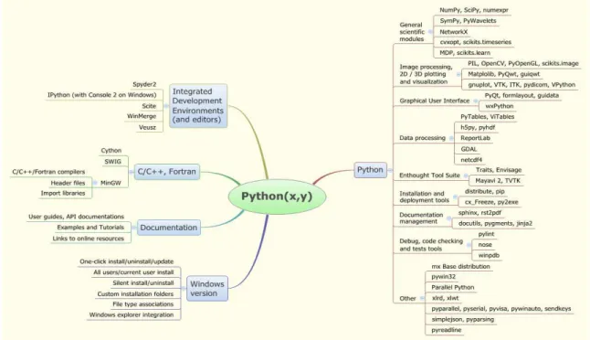
Figure 1.2: A full content of Python(x,y).

Optional libraries/editors which will be referenced in the course are: Spyder, Py2exe. They are already included in the Python(x,y) distribution.

Enthought/Canopy(Windows/Mac/Linux/Sun)

The Enthought full distribution is available for Windows, Mac, Linux and Sun Solaris. It is free for universities. Therefore use your university e-mail address when downloading this. There is also a lightweight distribution, which is free for all and which contains the essential libraries (Numpy/Scipy/Matplotlib) for this course except, again, Pygame. Go to :

http://www.enthought.com/

Download Enthought version 7.2 which contains Python 2.7. Then add pygame:

Current version of Pygame at the writing of this document is 1.9.1. Select the correct version for your OS and Python version.

Enthought has many libraries (see http://www.enthought.com/products/epdlibraries.php ) but not the Spyder editor nor Py2exe.

There is also a distribution for Apple (& Windows that is called Anaconda, but this will install 64-bit versions on 64-bit machines. The problem is that there is no 64-bit version of Pygame.

(13)

1.3.2 Customized installation of separate packages (Windows/Mac/Linux) If you do not want to use these large distributions, there is always the option to install Python and the modules yourself. Do this in the following order:

Download Python 2.7 for your OS from:

http://python.org/download/

For scientific computing, now download Numpy+Scipy for Python 2.7 from:

http://www.scipy.org/Download

For plotting then add Matplotlib for Python 2.7 from:

http://matplotlib.sourceforge.net/ (Select ‘Download’ in the text on the right side) For 2D moving graphics, keyboard and mouse input, now download pygame from:

This completes the set-up you need for this course. To start Python select ‘IDLE’ from the Python folder in the Start Menu. Or even better: create a Shortcut to this on your desktop, set the working directory to the folder where you want to keep your Python programs.

1.3.3 Documentation

IDLE has an option to Configure IDLE and add items to the Help menu. Here a link to a file or a URL can be added as an item in the Help pull down menu.

The Python language documentation is already included.

For Scipy and Numpy, downloading the .CHM files (‘chum-files’) of the reference guides onto your hard disk and linking to these files is recommended. They are available for download at:

http://docs.scipy.org/doc/

For Matplotlib both an online manual as well as a pdf is available at:

http://matplotlib.sourceforge.net/contents.html

Also check out the Gallery for examples but most important: with the accompanying source code for plotting with Matplotlib:

http://matplotlib.sourceforge.net/gallery.html

(14)

http://www.pygame.org/docs/

Another useful help option is entering ‘python’ in the Google search window followed by what you want to do. Since there is a large Python user community, you will easily find answers to your questions as well as example source codes.

1.3.4 Optional tools

A working environment, in which you edit and run a program is called an IDE, which stands for Integrated Development Environment. Which one you use, is very much a matter of taste. In the course we will use as an editor and working environment the IDLE program, because of its simplicity. This is provided with Python and it is easy to use for beginners and advanced programmers. Since it comes with Python, it is hence also available in both distributions. For larger projects or more advanced debugging, Spyder is recommended. Spyder is included in Python(x,y).

If you did the customized installation and you want to use Spyder, you first need to download PyQt from riverbanks (when you have the Enthought distribution, you already have this):

http://www.riverbankcomputing.co.uk/news

Then to download Spyder go to:

http://code.google.com/p/spyderlib/

Py2exe can be installed separately and is already included in Python(x,y) . How to install and use this is covered in the chapter on distributing your Python programs.

1.3.5 Configuring and using Python

First: Change Working Folder to My Documents\Python

In Windows, IDLE will start in the Python program directory (folder) and this will therefore also be your default working directory. This is dangerous because you may overwrite parts of Python when you save your own programs. Therefore make a shortcut on your Desktop in which we change the working folder to a more appropriate one. Right-click in the Start Menu on IDLE, select Copy and then Paste it on to your Desktop. Then right click Properties of this Shortcut and change the working directory to the folder where you want to keep your Python code (e.g. My Documents\Python).

Add links to your documentation of the Help menu

Start IDLE. Then if you have not already done so, select in the menu of the IDLE window, Options>Configure IDLE>General to add additional Help sources in the lower part of the property sheet. Download the documentation for Scipy (CHM files) and use the link to the pygame/docs site as well as the Matplotlib gallery.

(15)

In the IDLE window, named Python Shell, select File>New Window to create a window in which you can edit your first program. You will see that this window has a different pull-down menu. It contains “Run”, indicating this is a Program window, still called Untitled at first. Enter the following lines in this window:

print “Hello World!”

print “This is my first Python program.”

(if you would have chosen to use Python 3.x, you should add brackets around the texts and find another reader on the web, since we will use Python 2.x syntax in all our examples).

Now select Run>Run Module. You will get a dialog box telling you that you have to Save it and then asking whether it is Ok to Save this, so you click Ok. Then you enter a name for your program like hello.py and save the file. The extension .py is important for Python, the name is only important for you. Then you will see the text being printed by the program which runs in the Python Shell window.

After File>New Window, IDLE shows an editor window (right) next to the Shell window(left)

Switching off annoying dialog box “Ok to Save?”

By default, IDLE will ask confirmation for Saving the file every time you run it. To have this dialog box only the first time, goto Options>Configure IDLE>General and Select “No Prompt” in the line: At Start of Run(F5). Now, on a Windows PC, you can run your programs by pressing the function key F5. Now only the first time you run your program, it will prompt you for a locations and filename to save it, the next time it will use the same name automatically.

(16)

1.3.6 Spyder: a more advanced IDE

Though IDLE is a very useful IDE (Interactive Development Environment), there are some limitations:

- With large projects and many files it can become cumbersome to switch between different files

- Debugging facilities are limited

For this reason often another IDE is used for larger projects. There are many on the web. For scientific purposes the most popular one is Spyder. This comes with python(x,y) and many other distributions. An example of a screenshot of Spyder with some explanation is given below:

Spyder screenshot

Other features include inspecting data arrays, plotting them and many other advanced debugging tools.

Make sure to change the settings of file in the dialog box which will pop up the first time you run the file to allow interaction with the Shell. Then you have similar features to which IDLE allows: checking your variables in the shell after running your program or simply to testing a few lines of code.

My advice would be to first keep it simple and use IDLE for the basics. Use the print statement and the shell (to inspect variables) as debugger and occasionally www.pythontutor.com. Then later, for larger or more complex problems switch to Spyder.

(17)

1.4 Examples and exploration of the language

1.4.1 Temperature conversion: (PRINT, INPUT statement, variables) In the IDLE window, named Python Shell, select File>New Window to create a window in which you can edit your program. You will see that this window has a different pull-down menu. It contains “Run”, indicating this is a Program window, still called Untitled at first.

Enter the following lines in this window and follow the example literally. If you type 5 (so leave out the decimal point) instead of 5.0 the program might not work.

(If you want to make it a bit more interesting, and harder for yourself, you could make a variation on this program. In much the same fashion, you could try to make a saving/debt

interest calculator where you enter start amount, interest rate in percentage and number of years. To raise x to the power y, you use x**y)

Now select Run>Run Module. Depending on your settings, you might get a dialog box telling you that you have to Save it and then asking whether it is Ok to Save this, so you click Ok. Then you enter a name for your program like temperature.py and save the file. The extension .py is important for Python, the name is only important for you. Then you will see the text being printed by the program, which runs in the window named “Python Shell”:

(18)

Now let us have a closer look at this program. It is important to remember that the computer will step through the program line by line. So the first line says:

print "Temperature convertor Fahrenheit => Celsius"

The computer sees a print statement, which means it will have to output anything that comes after this statement (separated by commas) to the screen. In this case it is a string of characters, marked by a “ at the beginning and the end. Such a string of characters is called a text string or just string. So it put this on the screen. The computer will also automatically add a newline character to jump to the next line for any next print statement (unless you end with a comma to indicate you want to continue on the same line!).

Then this line is done, so we can go to the next one, which is slightly more complicated:

tempf = input("Enter temperature in degrees Fahrenheit: ") This line is a so called assignment statement, indicated by the “=” symbol. In general, it has the following structure:

variablename = expression

In our example it tells the computer that in the computer’s memory a variable has to be created with the name tempf.

To be able to do this, the computer first evaluates the expression on the other side of the “=” sign to see what the type of this variable has to be. It could for example be a floating point value (float type) or a round number (integer type), a serie of characters (string) or a switch (boolean or logical). It then reserves the required amount of bytes, stores the type and the name. If the name already exists, then this old value and type are first to avoid problems later on.

(19)

The computer evaluates the expression. The outcome is stored in memory and can be used later in other expressions by using the variable name. To do this, the computer maintains a table in its memory with the value of a variable, its name and its type.

a = 2

For numbers there are two types: integers and floats. Integers are whole numbers, used to count something or as an index in a table. Floats are numbers with a floating point and can be any value. Python looks at the expression to determine the type:

2 => integer type -4 => integer type 3*4 => integer type 2.0 => float type 0. => float type 1e6 => float type 3*4. => float type

Now let us have a look at the expression, This is not a simple one. The expression in our example has the following structure:

functionname ( argument )

Python knows this is a function because of the brackets. In this case, the name of the function is which is used is input( ), one of the standard functions included in the Python language. (Later we will also use functions which we have defined ourselves!)

Most functions do some calculations and yield a value. Example of these functions are abs(x) for the absolute value (modulus) of x or int(x) which will truncates the float x to returns an integer type. The int( ) function is one of the type conversion functions:

int(3.4) => integer with value 3 int(-4.315) => integer with value -4 float(2) => float with value 2. float(0) => float with value 0.

But some functions are complete little programs in itself. The input-functions for example does more: it can be called with one argument, which will be printed on the screen, before the user is prompted to enter a value. When the user presses enter, the value is read, the type is determined

(20)

and this is returned as the result by the input function. So in our case, the text Enter temperature in degrees Fahrenheit: is printed and the user enters something (hopefully a number) and this is then stored as an integer or floating point number in a memory location. We call this variable tempf.

The next line is again an assignment statement as the computer sees from the equal sign “=”: tempc = (tempf-32.0)*5.0/9.0

Here a variable with the name tempc is created. The value is deduced from the result of the expression. Because the numbers in the expression on the left side of the equal sign are spelled like “5.0” and “32.0”, the computer sees we have to use floating point calculations. We could also have left out the zero as long as we use the decimal point, so 5./9. would have been sufficient to indicate we want to use floating point values.

If we would leave them out, the result might be an integer value, which means that every

intermediate value is truncated (so cut off behind the decimal point) which would mean the result of the expression would be zero, as 5/9 would yield zero as result in integer arithmetic!

When this expression has been evaluated, a variable of the right type (float) has been created and named tempf, the computer can continue with the next line:

print tempf," degrees Fahrenheit is",int(tempc),"degrees Celsius"

This line prints four things: a variable value, a text string, an expression which needs to be evaluated and another text string, which are all printed on the same line with each comma a space character is automatically inserted as well. The int function means the result will be truncated (cut off behind the decimal point). Better would have been to use:

int(round(tempc))

What do you think the difference would have been? (check section 2.8).

Try running the program a few times. See what happens if you enter your name instead of a value.

1.5.2 Example: a,b,c formula solver (IF statement, Math functions) Now create a new window and enter the program below

import math

print "To solve ax2 + bx + c = 0 :" a = input("Enter the value of a:")

(21)

b = input("Enter the value of b:") c = input("Enter the value of c:") D = b**2 - 4.*a*c

x1 = (-b - math.sqrt(D)) / (2.*a) x2 = (-b + math.sqrt(D)) / (2.*a)

print "x1 =",x1 print "x2 =",x2

Run this program and you will see the effect. Some notes about this program:

- note how ** is used to indicate the power function. So 5**2 will yield 25. (Using 5*5 is faster by the way.)

- the program uses a function called sqrt() This is the square root function. This function is not a standard Python function. It is part of the math module, supplied with Python. Therefore the math module needs to be imported at the beginning of the program. The text math.sqrt() tells Python that the sqrt() function can be found in the imported math module

- After you have run the program, you can type D in the shell to see the value of the discriminant. All variables can be checked this way.

Also, note the difference between text input and output. The line print is a statement, while input is used as a function returning a value, which is then stored in a variable. The argument of input-function is between the brackets: it’s a prompt text, which will be shown to the user before he enters his input.

There is one problem with our program. Many times it will stop with an error because the discriminant D is negative, resulting in an error with the square root function.

To solve this, let us try adding some logic to the program, see below. Adapt your program to match this precisely, note the margin jumps (use TAB-key) in the IF statement, which is called indentation.

from math import sqrt

print "To solve ax2 + bx + c = 0 ," a = input("Enter the value of a:") b = input("Enter the value of b:") c = input("Enter the value of c:") D = b**2 - 4.*a*c

(22)

print "This equation has no solutions." else: x1 = (-b - sqrt(D)) / (2.*a) x2 = (-b + sqrt(D)) / (2.*a) print "x1 =",x1 print "x2 =",x2

Now the program first checks whether D is negative. If so, it will tell you that there are no solutions.

- Note the structure and syntax(=grammar) of the if-else statement. A colon ( : ) indicates a block of code will be given, so it acts as a ‘then’. The block is marked by the indented part of the code,.

- When it jumps back to the margin of the beginning to indicate the end of this block of code, an ‘else’ follows, again with a colon and an indented block of code.

- It also uses a different way to import the sqrt function from the math module. Note the difference in syntax in both the line with the import statement as well as the line where the sqrt function is used.

Assignment 1.1:

Adapt the program so that it calculates the hypotenuse c of a rectangular triangle for rectangular sides a and b as entered by the user, using Pythagoras formula.

Assignment 1.2:

Now adapt the program so that it determines the maximum value of given numbers a,b,c and d. Use the algorithm described before. Translate this into Python code using the example above and run it

Assignment 1.3***:

Change the program in a way that it solves a third order polynomials written as:

3 2

0 x +ax + + =bx c

The user enters the values of a, b and c. And the program prints the solutions for x. Find the required formulas by searching for “formulas to solve polynomial functions nth degree”.

1.5.3 Example: using lists and a for-loop

Now let us have a look at a program which is slightly more complex. First explore the range function. Go to the Python shell and type the following lines to see how the range function works.

(23)

range(2,22,2) range(5,1,-1)

What do you notice? If you do not see its logic, try a few values yourself. Some things you probably have noticed:

- It produces a list of integers separated by a comma in between square brackets: [2, 3, 4, 5]

- the range-function has three arguments start, stop and step The stop is always required, but start en step are optional.

- the default start value is zero - the default step value is one

- the start value is included in the list - the stop value is not included in the list

This result is in fact a new variable type: a list . You can regard this as a table: a = [ 7, 3, -1, 3]

Indexing of the list starts with zero, so a[0] will return in the first value (7) and a[3] the last one (3).

For the next example code we will use the website http://www.pythontutor.com . Go to this site and on the start page cick “Start using..”, clear the source edit window and enter this program in the window (also mind the layout (use tab to move the margin right!)

a = 9

for i in range(1,11): x = i*a

print i,"x", a,"=",x

print

print "Ready."

Now click “Visualize execution” and then click “Forward” a few times to see what happens. On the right side of the edit window you can see what happens in the memory of the computer. Next, you see the output window, with the text the user of the program will see:

(24)

Can you explain what the computer does? Why he jumps back? How he knows which part of the code to repeat and which not? Do you notice what happens to the value of i when it jumps back to the for-statement? What happens when i is equal to 10?

This is called a for-loop: i is assigned the first value of the list (in this case the list made by the range function) and after it has completed the indented block of code, it jumps back and assigns the next value of the list until it has reached the end of the list. If there are no more value for i, so after the last value it continues the code and does not jump back, the variable i now has the final value (10, because 11 is not included in the list generated by the range-function. See also the program below, what will this program do? Which integer do you think the len() function returns?

lst = [ 40. , 5. , 13., 1., 5. ]

for i in range(len(lst)): print 2*lst[i]

Notice the difference in syntax between calling a function in Python: sqrt(D)

len(a)

range(1,11)

and the use of a list with indices:

a[0] # to get the first element use index zero!

lst[i] # when i=1, you get the second element, etc.

You can see that Python knows whether something is a list or a function based on the type of brackets used!

(25)

Ttab = [0.0, 10.0, 20.0, 30.0, 40.0, 50.0, 60.0, 70.0, 80.0, 90.0, 100.0] Htab = [0.06,42.1, 84.0, 125.8,167.5,209.3,251.2,293.0, 335.0, 377.0,419.1]

n = len(Ttab) # Length of list

T = input("Enter temperature in degrees Celsius:")

for i in range(n-1):

if T >= Ttab[i] and T < Ttab[i+1]:

print "H is between",Htab[i],"and",Htab[i+1]

Note the two indentations: one for the for-loop, the next for the if statement.

A unique feature of Python is that the same list can store different types of variables: b = [2, ”Hello there!”, 3.141565 , 2, 10.0, True]

This assignment of b is a valid list, and it consists of a mix of variable types: floats, integers, a string and a Boolean(logical)

You even store lists in a list:

c = [ [2, 3, -1] , [3, 4, 0] , [7, 1, 1] ]

And the result is basically a two dimensional table, as we can see by showing some values of this table in the Python shell (first type the assignment statement above):

>>>c[0]

[ 2, 3, -1 ]

>>>c[2][0] 7

The second c[2][0] basically means, from left to right: the third element of c (which is a list)and then the first element of that list.

Through with this format it is easy to select a row, but selecting a column is only possible with a for loop. Below there are two ways to go through a two dimensional list to pick a column, What would be advantages of each method?

The first method is to have an integer run through a list of integers (so whole numbers) as generated by the range function: [0,1,…..len(people)-1] Remember the end value given in the range function will not be included in the range functions resulting list. These are exactly the indices for the list as this also starts with 0 and ends with its length minus one.

# Database: one statement can cover more program lines people = [ ["Jan", 18, "Delft"], \

(26)

["Piet", 20, "Leiden"], \ ["Kees", 19, "Amsterdam"], \ ["Klaas",34, "Utrecht"], \ ["Victor",22,"Leeuwarden"] ] iname = 0 iage = 1 icity = 2

# Show first two columsn of table for i in range(len(people)):

print people[i][iname],"is",people[i][iage],"years old."

The above way will work in most other programming languages as well. A unique feature of python is that a list of any type can be used as the counter (or as we call it: iterator) in the loop. The variable person will get each value from the list people. As people is a list of lists, person will first be the first element from people: ["Jan", 18, "Delft". Then, when the block of code that is in the loop has been executed with this value for person, the next value of people will be used: ["Piet", 20,

"Leiden"] and so on, for as long as the list people lasts:

# Database: see how one statement can cover more program lines # (within a list definition, without the backslash is also ok) people = [ ["Jan", 18, "Delft"], \

["Piet", 20, "Leiden"], \ ["Kees", 19, "Amsterdam"], \ ["Klaas",34, "Utrecht"], \ ["Victor",22,"Leeuwarden"] ] iname = 0 iage = 1 icity = 2

# Show first two columsn of table for person in people:

print person[iname],"is",person[iage],"years old."

Lists are often created by appending values at the end of the list, using the append function, which comes with the list-type and has a special syntax (varname.function), similar to how we use functions from a module, which we will later see more often. Such a function, which is called by a dot after the variable name is called a method, in this case of the list object (i.e. the list type).

Try this bit of code:

debt = [] rate = 1.03

(27)

x = 30000.

for i in range(30): debt.append(x) x = x*rate

print debt

Now try to change the line with the append function in: debt.append([i,x])

and see what the effect is (and what the debt is after 30 years of only 3% interest!). Could you think of a way to make the output look better, using a for-loop, list-indices, the e.g. the round( ) function (see section 2.8)?

1.5.4 While loops

The final basic statement which will complete your basic Python vocabulary is the while statement. It has been formally proven that with IF and WHILE you can program any logic you can think of. The FOR loop is basically a special case of the while-loop, for convenience. So how does the while loop work? It is basically an IF statement which will repeat the indented block of code until the condition becomes false. See the example below:

x = 0.

while x+5>x*x: print x x = x+1

What do you think the output of this program will be? The flow chart of this program would look like this:

Or see how this while-loop finds the right spot in a table to interpolate: # Enthalpy of water at 1 atmosphere

Ttab = [0.0, 10.0, 20.0, 30.0, 40.0, 50.0, 60.0, 70.0, 80.0, 90.0, 100.0] Htab = [0.06,42.1, 84.0, 125.8,167.5,209.3,251.2,293.0, 335.0, 377.0,419.1]

n = len(Ttab) # Length of list

T = input("Enter temperature in degrees Celsius:")

i = 0

while T>Ttab[i+1] and i+1<n-1: i = i + 1

print "H is between",Htab[i],"and",Htab[i+1]

(28)

Hip = (1.-f)*Htab[i] + f*Htab[i+1]

print "My best guess is that H will be:",Hip

In the following example a while loop is used to find a value in a list: # List of brands and products

brands = ["Apple","Samsung","Airbus","Renault","Microsoft","Google"]

products = [["computers","tablets","cell phones","music"], ["Electronics"],

["Airliners","Transport aircraft"], ["Cars"],

["Software"],

["Search engines","Operating Systems"]]

# String input with raw_input function

br = raw_input("Give a brand name:")

# Initialize loop parameters: counter and boolean/logical variable i = 0

found = False

# Can you see why we use the len(brands)–1 here? while i<len(brands)-1 and not found:

if not brands[i] == br: i = i + 1

else:

found = True

# Show result of search loop

if found:

print "They make:",products[i] else:

print "I don't know the brand",br,”!”

1.5.5 More modules

Python comes with many handy features built-in as modules. To be able to access these from your program, simply put an import statement at the beginning. Then in your program simply type the module name followed by a period and the function name. In this way you can access all functions inside this module. Some examples are given in this section.

Type in the shell help(“time”) or help(“time.localtime”) and try to see what happens in the program below. It uses the time module to get current local time and date as integers (whole numbers).

import time

# Get local time & date t = time.localtime()

(29)

hour = t[3] mins = t[4] secs = t[5] date = t[2] month = t[1] year = t[0]

# Or use the time struct . See help(“time.time”) hour = t.tm_hour mins = t.tm_min secs = t.tm_sec date = t.tm_mday month = t.tm_mon year = t.tm_year

Or the random number generator from the moduel named random (in the shell type

help("random.random") and help("random.randint") to get more information: import random

# Two ways to get a number 1-6 die = int(random.random()*6)+1 print die

die = random.randint(1,6) print die

1.5.6 Finding your way around: many ways in which you can get help Using help(“text”) or interactive help()

If you wonder how you could ever find all these Python-functions and function modules, here is how to do that.

There are many ways to get help. For instance if you need help on the range function, in the Python shell, you can type:

help(“range”)

Which calls the help-function and uses the string to find appropriate help-information. Similarly to find methods of the list or string type, use:

help(“list”)

You can also use help interactively by typing help(), without arguments, and then type the keywords to get help, e.g. to see which modules are currently installed.

(30)

>>>help() help>math

And you will see an overview of all methods in the math module. There are some limitations to this help. When you will type append, you will not get any results because this is not a separate function but a part of the list object, so you should have typed

>>> help("list.append")

Help on method_descriptor in list: list.append = append(...)

L.append(object) -- append object to end

>>>

or list.append in the interactive help: >>> help()

Welcome to Python 2.7! This is the online help utility. …..

help> list.append

Help on method_descriptor in list: list.append = append(...)

L.append(object) -- append object to end

help>

Python documentation in Help Pull-down menu

So anther way is to use the supplied CHM-file, (compiled HMTL) via the Help-menu of the IDLE-windows: Select Help>Python Docs and you will find a good set of documentation, which you search in the “Index” or do a full text search (“Search”), see the screenshots on the next page:

(31)

(32)

Using the huge Python community

Python has a very large user community: conservative estimates say there are 3 to 5 million Python users and it’s growing fast as MIT, Stanford and many others use Python in their courses and exercises. It is also the most popular language among PhDs and IEEE calls it the standard for scientific computing.

So simply Googling a question (or error message) with the keyword Python (or later Numpy) in front of it as an extra search term will quickly bring you to a page with an example or an answer. For basic questions this might bring you to the same documentation as in the Help-menu which is at http://docs.python.org . You will also see that www.stackoverflow.com is a site, which will often pop-up, and where most questions you might have, have already been posed and answered: For instance, for “python append to a list” you will find:

http://stackoverflow.com/questions/252703/python-append-vs-extend

(Which shows that next to append there apparently is another method called extend which works with a list as an argument and apparently appends each element to the list.)

In general, thanks to the interactive Python Shell window, simply trying statements or program lines in the Python shell is a way to try what works as you intended. Or to check the value of variables after your still incomplete program has run.

To find bugs in your program, for small programs http://www.pythontutor.com can be helpful to what is going on inside the computer when your program runs. And of course using the print statement to see what a variable is, or where the computer gets stuck in your program, is always the first thing to try.

Be prepared that in the beginning the level of frustration might be high, but so is the reward when your program runs. And when you get experience, you will see how fast you can make working programs, not because you won’t create bugs, but because you will immediately recognize what went wrong. The nice thing of software is that it can always be fixed, so “trial and error” is an accepted way to develop programs. So do not be afraid to try things and play around with Python to get acquainted with the way it works.

In appendix A and appendix B a short overview of the Python statements and mpst important functions is given. In section 5.2 an overview of the math-functions is given. Having a copy of these pages at hand may be handy when starting Python. It will provide the keywords for you to look into the help-functions of Google searches.

Although we already touched upon most basic elements of the Python language, we have not seen all statements and types yet, so first go through the next chapters (discover the very useful while-loop, the string type and its methods and the Boolean/logical and slicing of strings and lists etc.). Just glance over these chapters to get the essence and then start making simple programs and study the paragraphs in more details when you (think you) need them. Programming has a steep learning curve at the beginning, so good luck with making it through this first phase. Once you have passed this, things will be a lot easier and more rewarding. Good luck!

(33)

2. Python syntax: Variables and functions

In this chapter we describe the building blocks which you need to write a program. First we have a look at variables. A variable is used to store data. But there are different types of data: numbers or bits of text for instance. There are also different data types of numbers And of course there are more data types than just text and numbers, like switches (called “booleans” or “logicals”) and tables(“lists”). The type of variable is defined by the assignment statement, the programming line giving the variable its name, type and value. Therefore we first concentrate the assignment statement and then the different data types are discussed.

2.1 Assignment and implicit type declaration

A variable is a memory location with a name and a value. You define a variable when you assign a value or expression to it. This expression also determines the type. The assignment statement is very straightforward:

variablename = expression

Example assignments of the four main types (which will be discussed in details in the following sections): Integers: i = 200 a = -5 Floats: in = 2.54 ft = .3048 spd = 4. alt = 1e5 Logicals: swfound = True prime = False Strings: name = “Jane” txt = “Hello world.” s = ‘abc’

2.2 Floats

Floats, commonly referred to as floating point variables, are used for real numbers. These are the numbers as you know them from your calculator. Operations are similar to what you use on a calculator. For power you use the asterisk twice, so xy is achieved by x**y.

(34)

One special rule with floats in programming is that you never test for equality. Never use the condition “when x is equal to y” with floats, because a minute difference in how the float is stored can result an inaccuracy, making this condition False when you expected otherwise. This may not be visible when you print it, but still causing two variables to be different according to the computer while you expected them to be the same. For example: adding 0.1 several times and then checking whether it is equal to 10.0 might fail because the actual result is approximated by the computer as 9.99999999 when it passes the 10. So always test for smaller than (<) or larger than (>). You can also use “smaller or equal to” (<=) and “larger or equal to” (<=).

2.3 Integers

Integers are variables used for whole numbers. They are used for example as counters, loop variables and indices in lists and strings. They work similar to floats but division results will be ‘floored’. This means that integers are always rounded off to the lower whole number (so truncated or cut off). For example:

a = 4 b = 5 c = a/b

print c

This will print zero in the screen and not 0.8. This is the source of many bugs: variable become integer by accident (the programmer forgets to add the decimal point), and strange result come out of th expressions because some intermediate value is rounded off to zero. So never forget the decimal point or using the float(0 conversion function when necessary!

A very useful operator with integers is the ‘ %’ operator. This is called the modulo function. You could also call it “the remainder” because it gives only remainder of a division. For example:

27%4 = 3 4%5 = 4 32%10 = 2 128%100 = 28

So to check whether a number is divisible by another, checking for a remainder of zero is sufficient:

if a%b==0:

print “b is a factor of a”

You can convert integers to floats and vice versa (since they are both numbers) with the functions int( ) and float( ):

a = float(i)

j = int(b) # Cut of behind decimal point

k = int(round(x)) # Rounded off to nearest whole number

The int( ) function will cut off anything behind the decimal point, so int(b) will give the largest integer not greater than b . These functions int( ) and float( ) can also take

(35)

strings (variables containing text) as an argument, so you can also use them to convert text to a number like this:

txt = “100” i = int(txt) a = float(txt)

2.4 Strings

Strings are variables used to store text. They contain a string of characters (and often work similar to a list of characters). These are defined by a text surrounded by quotes. These quotes can be single quotes or double quotes as long as you use the same character to start and end the string. It also means you can use the other type of quote-symbol inside the text. A useful operator on strings is the “+” which glues them together, This is very useful e.g in functions which expect one string variable (like the input function).

Example assignments:

txt = “abc” s = “”

name = “Jacco”+” M. “+”Hoekstra” (so the + concatenates strings) words = ‘def ghi’

a = input(“Give value at row”+str(i)) Some useful basic functions for strings are:

len(txt) returns the length of a string

str(a) converts an integer or float to a string

eval(str) evaluates the expression in the string and returns the number chr(i) converts ASCII code i to corresponding character

ord(ch) returns ASCII code of the character variable named ch

Using indices in square brackets [ ] allows you to take out parts of a string. This is called slicing. You cannot change a part of string but you can concatenate substrings to form a new string. This can be used to achieve the same thing:

c = “hello world”

c[0] is then “h” (indices start with zero)

c[1:4] is then “ell” (so when 4 is end, it means until and not including 4) c[:4] is then “hell”

c[4:1:-1] is then “oll” so from index 4 until 1 with step -1 c[::2] is then “hlowrd”

c[-1] will return last character “d” c[-2] will give one but last character ”l”

c = c[:3]+c[-1] will change c into “hel”+”d”=“held”

the string variable also has functions built-in, the so-called string methods. See some examples below (more on this in chapter 8).

(36)

a = c.lower() returns copy of the string but then in lower case

a = c.strip() returns copy of the string with leading and trailing spaces removed sw = c.isalpha()returns True if all characters are alphabetic

sw = c.isdigit()returns True if all characters are digits i = c.index(“b”) returns index for substring in this case “b”

For more methods see chapter 8 or 5.6.1 of the Python supplied reference documentation in the Help file.

(37)

2.5 Logicals/Booleans

Logicals or Booleans are two names for the variable type in which we store conditions. You can see them as switches inside your program. Conditions can be either True or False, so these are the only two possible values of a logical. Mind the capitals at the beginning of True and False when you use these words: Python is case sensitive. Examples of assignments are given below: found = False prime = True swlow = a<b outside = a>=b swfound = a==b

notfound = a!=b ( != means: not equal to)

notfound = a<>b ( <> also means: not equal to, but is old notation) outside = x<xmin or x>xmax or y<ymin or y>ymax inside = not outside

out = outside and (abs(vx)>vmax or abs(vy)>vmax) inbetween = 6. < x <= 10.

Conditions are a special kind of expressions used in statements like if and while to control the flow of the execution of the program. In the above statements, often brackets are used to indicate it is a logical expression.

To test whether two variables are the same, you have to use two equal signs. Two equal signs will check the condition and one equal sign assigns an expression to a variable name. For “is not equal to” both != as well as <> can be used, but != is preferred. With combined conditions with many “and”, “or” and “not” statements use brackets to avoid confusion:

not((x>xmin and x<xmax) or (y>ymin and y<ymax)) You can use logicals as conditions in if and while statements:

if inside:

print “(x,y) is inside rectangle”

while not found: i = i + 1

found = a==lst[i]

Note that if inside basically means: if inside==True and similarly while not found means while found==False .

(38)

2.6 Lists

2.6.1 What are lists?

Lists are not really an independent type but a way to group variables together. This allows you to repeat something for all elements of a list by using an index or by iterating through the list with the for-statement. This could be an operation, a search or a sorting action. Often it is useful to have a series of variables. Look at it as a table. An element of a list could be of any type, it can be an integer, float, logical, string or even a list! Special for Python is that you can even use different types in one list; in most programming languages this would not be possible. Both to define a list, as well as to specify an index, square brackets are used as in strings.

a = [ 2.3 , 4.5 , -1.0, .005, 2200.] b = [ 20, 45, 100, 1, -4, 5] c = [“arie”,”toos”,”bep”,”truus”] d =[[“Frederik”,152000.], [“Gert-Jan”,193000.], [“Alexander”,110000.]] e = []

This would make the variable a a list of floats, b a list of integers, c a list of strings. A list of lists as defined in d is basically a way to create a two-dimensional list. Finally e is an empty list. Accessing elements from the list is done as indicated below. Another way to make a list of numbers is using the range function. The range function can contain one two or even three arguments:

range(stop)

range(start,stop)

range(start,stop,step)

In all these cases start is the start value (included), stop is the value for which the block is not executed because for will stop when this value is reached. So it is an inclusive start but excludes stop. Another option is to enter a third argument, which is then is the step. The default start is 0, the default step is 1. Note that range( ) only works with integers:

range(5) equals [0,1,2,3,4]

range(5,11) equals [5,6,7,8,9,10]

range(5,11,2) equals [5,7,9]

(39)

2.6.2 Indexing and slicing Let's use the following list:

lst = [1,2,3,4,5,6,7,8,9,10]

If we now print elements we can use the indices in many ways. Using one index, indicating a single element:

lst[0] which holds value 1 lst[1] which holds value 2 lst[9] which holds value 10

lst[-1] last element, which holds the value 10 lst[-2] one but last element which holds the value 9

Here it can be seen that indices start at 0, just as with strings. And similar to strings, the function len( ) will give the length of a list and thus the not to reach maximum for the list. Slicing lists with indices also works just as for strings, with three possible arguments: start, stop and step. Only one index refers to one single element. Two arguments separated by a colon refer to start and stop. A third can be used as step. If you look at the lists that were made in the previous paragraph about lists you can see that:

a[1] will return a float 4.5

b[1:4] will return a list [45, 100, 1]

d[1][0] will return “Gert-Jan” (do you see the logic of the order of the indices?)

Adding and removing elements to a list can be done in two styles: a = a+[3300.] will add 3300. at the end of the list

a = a[:-2] will remove the last two elements of the list (by first copying the complete list without the last two elements, so not very efficient for large lists)

a = a[:i]+a[i+1:] will remove element i from the list, when it’s not the last one in the list

a = b + c will concatenate (glue together) two lists if b and c are lists Another way is to use the del (delete command) and/or functions which are a part of the list class. You call these functions by variablename.functionname( ) so a period between

variablename and functionname. Some examples:

a.append(3300.) add 3300. at the end of the list named a a.remove(3300.) removes the first element with value 3300.

(40)

del a[-1] removes the last element of list named a

a = a[:3]+a[4:] will remove the 4rd element of the list named a Slicing

The last example line uses the slicing notation (which can also be used on strings!). Slicing, or cutting out parts of a list is done with the colon. The notation is similar to the range arguments: start:stop and optionally a step can be added as third: start:stop:step. If no value is enter as start, the default value is zero. If no value is added as end the default value is the last. De default step is 1. Negative values can be used to point to the end (-1 = last element, -2 is one but last etc.). Using the original definition of lst this will give:

lst = [1,2,3,4,5,6,7,8,9,10]

lst[:3] first three element index 0,1,2: [1,2,3] lst[:-2] all except last two elements

lst[4:] all elements except the first four: except elements nr 0,1,2,3 lst[::2] every second element so with index 0,2,4, until the end Other useful functions for lists:

b.index(45) will return the index of the first element with value 45 len(d) will return the length of the list

min(a) will return the smallest element of the list variable a max(a) will return the largest element of the list variable a sum(a) will return the sum of the elements in the list variable a

2.6.3*** Lists are Mutable: risks with multiple dimensions list creation You can quickly build a one dimensional list with 5 elements like this:

>>> a=5*[0] >>> a [0, 0, 0, 0, 0] >>> a[1]=1 >>> a [0, 1, 0, 0, 0] >>>

Warning: This only works with one dimensional arrays, see what happens when you try it with lists of lists, so two dimensional lists:

>>> a=3*[3*[0]] >>> a

[[0, 0, 0], [0, 0, 0], [0, 0, 0]]

>>> a[0][1]=1 >>> a

(41)

>>>

So we only change the second element of the first row, but surprisingly all rows (all lists) have their second element changed into 1!

In general you could say, simply avoid this. But for the people who really want to know what is going on: In www.python.tutor.com we can see the difference. Imagine we will run the following code:

a = 3*[0] b = 3*[a] c = 3*a

d = 3*[3*[0]]

Then in the computer’s memory, this is the result:

When using one dimensional lists with the star-sign (so for example *a or *[0]), it will be an expression, evaluated and taken as a value and hence create a new list. Examples of this are how the list a and d are created. But normally in Python a list is seen as an object, which means it will just be copied by reference (a pointer to the same object, to the same memory location) will be used. This causes the at first sight strange behavior.

To avoid this confusion (and ignore this difference), it is better to build a two dimensional array with append in a for-loop:

a=[]

for i in range(3): a.append(3*[0]) a[0][1] = 1

(42)

print a

Which will result in the following output:

[[0, 1, 0], [0, 0, 0], [0, 0, 0]]

But this code:

a=[] b=[0,0,0] for i in range(3): a.append(b) a[0][1] = 1 print a

This only slightly different code will result in the problematic output again:

[[0, 1, 0], [0, 1, 0], [0, 1, 0]]

So 3*[0] is an expression, just like integer variables and float variables. But because b is a list-object and passed on by reference to the memory location.

In general, using append with non-list arguments is a safe method. This is because most variable types (floats, integers, strings) are passed on as value. They are called immutable. Expressions are also passed on as a value. List objects (like most objects) are called mutable and will be passed on as a reference to a memory location and hence can be changed by the function that is called.

Here are two ways to quickly create a two-dimensional list without the risk of creating pointers to the same list:

First create a one dimensional list, then replace each element by a list: a=3*[0]

for i in range(3): a[i]=3*[0] a[0][1] = 1

print a

Or with nested loops, create a fresh, new list (as a row) and then append this: a=[] for i in range(3): row = [] for j in range(3): row.append(0) a.append(row) a[0][1] = 1 print a

(43)

Both will give this output, indicating that a indeed consists of three independent lists:

[[0, 1, 0], [0, 0, 0], [0, 0, 0]]

So creating the variable row or he list a lement a[i] every time anew, is the safest way to avoid all appended lists pointing to the same memory location. If you are not sure, test a simple example in the above way: change one element and see the effect by printing the list. Or use

www.pythontutor.com to see what is going on in the computer’s memory.

2.6.4 List methods

An advantage of lists are the methods that come with it. These are functions which you call with a period after the variable name (just like append). An example is the sort function:

>>> a=[2,10,1,0,8,7] >>> a.sort()

>>> a

[0, 1, 2, 7, 8, 10]

As we can see the function sort() (recognizable as a function because of the brackets) sorts the list a. This is special function in that is changes the actual source list instead of creating a sorted copy. Most methods will give the result of the function and leave the original intact. Example are the method index and count. Index will give the index of the first occurrence of the value. Count will give the total number of occurrences:

>>> a = [3,1,8,0,1,7] >>> a.count(1) 2 >>> a.index(1) 1 >>> a.index(9)

Traceback (most recent call last): File "<pyshell#23>", line 1

a.index(9)

ValueError: 9 is not in list

>>>

How would you make a program which will the index of the first occurrence but also avoids the error message if it is not found by simply printing -1?

Programming and Scientific Computing in