R., & Muller, H-G. (2018). Functional principal component analysis for
identifying multivariate patterns and archetypes of growth, and their
association with long-term cognitive development. PLoS ONE, 13(11),
[e0207073]. https://doi.org/10.1371/journal.pone.0207073
Publisher's PDF, also known as Version of record
License (if available):
CC BY
Link to published version (if available):
10.1371/journal.pone.0207073
Link to publication record in Explore Bristol Research
PDF-document
This is the final published version of the article (version of record). It first appeared online via Public Library of Science at https://journals.plos.org/plosone/article?id=10.1371/journal.pone.0207073 . Please refer to any applicable terms of use of the publisher.
University of Bristol - Explore Bristol Research
General rights
This document is made available in accordance with publisher policies. Please cite only the published
version using the reference above. Full terms of use are available:
Functional principal component analysis for
identifying multivariate patterns and
archetypes of growth, and their association
with long-term cognitive development
Kyunghee Han1, Pantelis Z. HadjipantelisID1, Jane-Ling Wang1, Michael S. Kramer2,
Seungmi Yang2, Richard M. Martin3,4, Hans-Georg Mu¨ ller1
*
1 Department of Statistics, University of California Davis, Davis, California, United States of America, 2 Departments of Pediatrics and of Epidemiology, Biostatistics and Occupational Health, McGill University, Montreal, Canada, 3 Bristol Medical School, Population Health Sciences, University of Bristol, Bristol, United Kingdom, 4 National Institute for Health Research Bristol Biomedical Research Centre, University Hospitals Bristol NHS Foundation Trust and the University of Bristol, Bristol, United Kingdom
Abstract
For longitudinal studies with multivariate observations, we propose statistical methods to identify clusters of archetypal subjects by using techniques from functional data analysis and to relate longitudinal patterns to outcomes. We demonstrate how this approach can be applied to examine associations between multiple time-varying exposures and subse-quent health outcomes, where the former are recorded sparsely and irregularly in time, with emphasis on the utility of multiple longitudinal observations in the framework of dimension reduction techniques. In applications to children’s growth data, we investigate archetypes of infant growth patterns and identify subgroups that are related to cognitive development in childhood. Specifically, “Stunting” and “Faltering” time-dynamic patterns of head circumfer-ence, body length and weight in the first 12 months are associated with lower levels of long-term cognitive development in comparison to “Generally Large” and “Catch-up” growth. Our findings provide evidence for the statistical association between multivariate growth patterns in infancy and long-term cognitive development.
Introduction
Objective of the study
The link between deficient growth in infancy and later life cognitive performance degradation has been widely accepted [1–3]. Stunting and faltering during infancy, or early childhood, are
associated with reduced cognitive ability in later age performance [4,5], and these growth
pat-terns have been the subject of extensive investigation [6–9]. In most of the previous work, investigators have studied this association by examining single growth indicators, for example head circumference [10] or body weight [11]. In particular, [12] examined how cognitive
a1111111111 a1111111111 a1111111111 a1111111111 a1111111111 OPEN ACCESS
Citation: Han K, Hadjipantelis PZ, Wang J-L,
Kramer MS, Yang S, Martin RM, et al. (2018) Functional principal component analysis for identifying multivariate patterns and archetypes of growth, and their association with long-term cognitive development. PLoS ONE 13(11): e0207073.https://doi.org/10.1371/journal. pone.0207073
Editor: Rhonda D. Szczesniak, Cincinnati Children’s
Hospital Medical Center, UNITED STATES
Received: June 13, 2018
Accepted: October 24, 2018 Published: November 12, 2018
Copyright:©2018 Han et al. This is an open access article distributed under the terms of the
Creative Commons Attribution License, which permits unrestricted use, distribution, and reproduction in any medium, provided the original author and source are credited.
Data Availability Statement: The PROBIT data
cannot be shared based on contractual terms in the participant consent agreement and inquiries can be made to Dr. Mourad Dahhou (Mourad.
[email protected]), a representative of the data access committee for the PROBIT study in the McGill University Health Center.
Funding: This study was supported by the Bill &
development of children in Vietnam is associated with pre-defined growth features at age 1 year. While features such as stunting, underweight, wasting and small head circumference were examined, the previous analysis was based on one growth modality, for example body length or weight.
We propose a straightforward way to combine multiple growth indicators under a single framework. Our approach provides a comprehensive assessment of the potential risk in terms of cognitive development using longitudinal information from growth patterns of several growth modalities. Specifically, we demonstrate a data analysis procedure that combines mea-surements from three commonly recorded time-varying growth traits, head circumference, body length and body weight. We then identify growth patterns that can be associated with subsequently measured full-scale IQ (Wechsler abbreviated scale of intelligence, WASI). The simultaneous consideration of multiple trajectories is a main novel feature of our approach.
We also devise a simple method to learn archetypal growth patterns from data and examine their association with subsequent IQ outcomes. Our methods assess multiple growth indica-tors nonparametrically without the need of prior growth charts [13]. Using a functional data
analysis (FDA) framework [14,15], the proposed methodology combines multiple growth
indicators and identifies data-driven clusters of infants according to their growth profiles. Recently, [16] and [17] considered quantile contour estimation of functional principal compo-nents (FPC) with emphasis on analysis for growth curves, but only with a single growth trajectory sample. In a related approach, [18] focused on finding subjective-specific warping functions to extract common features among multivariate growth traits. In contrast to existing approaches, we profile multiple growth patterns in terms of archetypal analysis [19–21], where we implicitly assume that extreme growth patterns can be used to represent individual growth curves in the sample through convex combination.
Our findings from applying the proposed methodology to the PROBIT growth study
cohorts [22,23] suggest that the proposed methodology is capable of identifying infant
sub-groups that differ in a statistically significant way in terms of the average level of associated IQs and thus can serve as a useful tool for identifying subgroups at risk of impaired cognitive development.
Data description
The data were collected as part of WHO’s Promotion of Breastfeeding Intervention Trial
(PROBIT) in the Republic of Belarus [22,23]. They include growth measurements taken
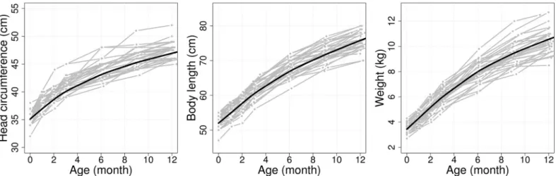
dur-ing the infancy of full term babies who weighed at least 2.5kg at birth among 17,045 total sub-jects. The physical traits recorded are head circumference, body length and body weight which were measured six times during the first year after birth. However, the sampling schedules were not strictly followed and some children did not have a full set of six measurements, the
data are best characterized as irregularly sampled longitudinal observations and seeFig 1. For
example, about 5.5% of the children have less than six measurements. For children with com-plete records, average measurement times were approximately 1.05 (0.12), 2.05 (0.13), 3.11 (0.24), 6.12 (0.31), 9.12 (0.34) and 12.10 (0.21) months after birth, where standard deviations at each visit are given in parentheses. We also refer to the design plot for measurement times during the first year in [13], which demonstrates the extent of sparsity and irregularity of the observation schedules over the first year after birth. The cognitive ability of children was assessed using the WASI score of the full-scale IQ measured at 6.5 years.
In addition to time-varying growth traits, a multitude of demographic covariates were also recorded. These covariates were used in later stages to control for potential confounding effects including socio-demographic factors. For example, children whose parents attended article contents are the sole responsibility of the
authors and may not necessarily represent the official views of the Bill & Melinda Gates Foundation or other agencies that may have supported the primary data studies used in the present study.
Competing interests: The authors have declared
university have higher IQ measurements on average than children whose parents did not to complete high-school education. These covariates are known to affect later age IQ throughout a child’s infancy [24–27]. Other covariates included the sex of the child, maternal and paternal education levels, maternal and paternal age-at-birth, maternal smoking during pregnancy, duration of exclusive breast feeding and the hospital where the child was born. The sample size
after preprocessing wasn= 12,809 children, whose data were analyzed in our study. For details
of data records and preprocessing, we refer to [13] and [22].
Methodology
Functional principal component analysis
LetXi(t) be a realization of a time-varying traitX(t) for thei-th subject, 1�i�n, at each time
pointt2T. Assuming independent measurements between subjects and that theXi(t) have
smooth trajectories over timet, we apply functional principal component analysis (FPCA) to
decompose patterns of temporal variation. A basic feature of FPCA is that the time-varying
trait of thei-th subject admits the Karhunen-Loève expansion [28–30]
XiðtÞ ¼mðtÞ þX k�1
xik�kðtÞ; ð1Þ
whereμ(t) = EX(t), and theξikare uncorrelated random variables with mean zero and variance
λksatisfyingλ1�λ2� � � �. Here inEq (1), theξikare thek-th FPC scores of thei-th subject,
associated with the eigenfunctionϕkfor allk�1. For theoretical background on FPCA and
related techniques, see [15,31–36].
In longitudinal studies, however, measurements of time-varying traits are only available
atNisuccessive time points, sayti1 <� � �<tiNi, for thei-th subject. We note that the set of
time pointsfti1;. . .;tiNigmay differ among thensubjects andNimay be small. FPCA for
lon-gitudinal data has been widely investigated [14,37–40]. Specifically, [41,42] proposed a
tech-nique to perform FPCA for sparse longitudinal data, based on principal components analysis through a conditional expectation (PACE) scheme. Specifically, we consider sparse and noisy Fig 1. Irregular and sparse longitudinal observations from the PROBIT data. Head circumference (HC, left), body length (LN, middle) and weight (WT, right) are
illustrated for a random selection of 30 subjects (gray) out of about 12,800 total children, along with estimated mean curves for each longitudinal trait (black solid lines).
longitudinal observationsX~ij¼XiðtijÞ þ�ij, instead of continuous and unperturbed
observa-tions of time-varying traitsXi(t), where the�ijare independent mean zero measurement errors.
By assuming thatξikand�ikfollow a joint normal distribution, the best linear predictors of the
FPC scoresξikare given by
^ xik¼l^k�^> ikS^ 1 ~ Xið ~ Xi ^μiÞ; ð2Þ whereX~i¼ ðX~i1;. . .;X~iNiÞ >
are longitudinal observations,μ^i¼ ðm^ðti1Þ;. . .;m^ðtiNiÞÞ
>
are the
estimates of mean vectors ofEX~i, andS^X~
iis the estimatedNi×Nivariance-covariance matrix
ofSX~
iwith (j,ℓ)-elements given byCovð
~
Xij;X~i‘Þ. Also,ðl^k;�^kðtÞÞ,k�1, are pairs of
estima-tors for eigenvalues and eigenfunctions, which are the solutions of the following equations
with respect to (λk,ϕk(t)), Z T Gðs;tÞ�kðsÞds¼lk�kðtÞ ðk¼1;2;. . .Þ; subject to lk�lkþ1 and Z T �kðtÞ�‘ðtÞdt¼ ( 0 ðk6¼‘Þ 1 ðk¼‘Þ ; ð3Þ
whereG(s,t) = Cov(X(s),X(t)) is the auto-covariance function ofX, so that we may write
^
�ik¼ ð�^kðti1Þ;. . .;�^kðtiNiÞÞ >
; see [43] and [15] for comprehensive overviews on FDA and recent developments in the interface between FPCA and longitudinal data.
Once we have estimated eigenfunctions�^kðtÞthrough the PACE method inEq (2),
longitu-dinal patterns ofX~ican be summarized by the corresponding FPC scoresx^ik. In fact,
unob-served time-varying traitsXi(t) can be reconstructed asX^iðtÞ ¼m^ðtÞ þ
PK
k¼1^xik�^kðtÞ, followed
by the representation in Eqs(1)and(3)with a cut-off valueK�1. The truncation pointKcan
be chosen as the smallest value satisfyingPKk¼1^lk=P‘�1^l‘�kfor a given 0<κ<1, so that a
fractionκof variance is explained (FVE), see [15,30]. The infinite dimensional functionsX^i
will then be represented byK-vectorsð^xi1;. . .;x^iKÞ>, which provides the required dimension
reduction.
Identification of outlying subjects
To study archetypes in the multivariate data analysis framework, we cluster longitudinal
obser-vationsX~iinto subgroups based on trajectory patterns of reconstructed time-varying traits
Xi(t). Time-varying traits are recovered by the first few FPC scores with high fraction of
vari-ance explained (FVE). In practice, the first two FPC scores produce relatively clear
discrimina-tion of the data characteristics in many sparse and irregular longitudinal studies [41,42,44,
45]. As an exploratory illustration tool for outlier detection in multivariate data analysis, the bagplot [46] was introduced as a generalization of the univariate boxplot. In the bagplot, half-space location depth [47] is usually adopted so that the multivariate data points are ordered
by an extended notion of univariate rank. The halfspace location depthDðx;XnÞof a point
x¼ ðx1;. . .;xKÞ >
2RKoverK-variate dataX
n¼ fξi 2R
K : 1�i�ngis defined by the
smallest number ofξicontained in any halfspace with boundary line passing x. Then, data
points can be ordered by depth, that isDðξi;XnÞ �Dðξi0;XnÞ, 1�i6¼i0�n. For modern
In this study, for the purpose of providing flexible inference based on sparse and irregularly observed functional and longitudinal data, we utilize the highest density region (HDR) as in
[50] and [51]. We consider the (1−α)-HDR for theK-variate data defined by
Rξ
ð1 aÞ ¼ fx2RK
:fξðxÞ �fag ð0<a<1Þ; ð4Þ
wherefξis the joint density of a random vectorξ= (ξ1,. . .,ξK)>and
fa ¼ arg max y>0 : Z RKfξðxÞ � IðfξðxÞ �yÞdx�a � � ð5Þ
in Eqs(4)and(5), respectively. Takingα= 0.05 yields a support region where observations are
expected to fall with at least 95% probability. We also note that the HDR captures the nature of the distribution of the data like location, scale, correlation and tail information in a flexible
man-ner. [52] proposed a kernel-type estimator ofRξð1 aÞ, wheref
ξandfαare replaced by kernel
density estimators, respectively. For example, one can use^fξðxÞ ¼n
1Pn i¼1
QK
k¼1Lhkðxik xkÞ
with bandwidthshk>0, whereLh(v) =L(v/h)/his a scaled version of a baseline kernelLthat is a
probability density function with finite variance. The kernel estimatorR^ð1 aÞofRð1 aÞ
also enjoys level information of the joint densityfξ. We identify (100×α)% extreme subjects in a
sample as those falling outside ofR^ð1 aÞ. For densely observed functional data, recent studies
have investigated several measures of functional outliers, such as band depth and extremal depth for functional data [53–55].
Joint feature extraction from multiple time-varying traits
In this subsection, we describe how we perform dimension reduction for multivariate
longitudi-nal observations by employing the covariance structure between multiple traits. UsingEq (1)and
the FVE method introduced in the previous subsection, letX�;½j�ðtÞ ¼PK½j�
k¼1x ½j� k�
½j�
kðtÞbe truncated
versions of the original time-varying traitsX[j](t) using only the firstK[j]eigenfunctions, where
�½kj�ðtÞis thek-th eigenfunction of thej-th trait, 1�j�d, 1�k�K[j], and letz½kj� ¼xk½j�=ðl½kj�Þ1=2
denote the standardizedk-th FPC score of thej-th longitudinal trait, respectively. Then the
functional covariance structure among the truncated time-varying traits (X�,[j]
(t):1�j�d)
can be reduced to the variance-covariance matrix ofðz½j�
k : 1�k�K ½j�;1�j�dÞ. Indeed, CovðX�;½j�ðsÞ;X�;½m�ðtÞÞ ¼PK½j� k¼1 PK½m� ‘¼1 ðl ½j� kl ½m� ‘ Þ 1=2 Covðz½kj�;z½‘m�Þ� ½j� kðsÞ� ½m� ‘ ðtÞ, 1�j6¼m�d. This
suggests to apply conventional principal component analysis (PCA) on the vector of standardized
marginal FPC scoresðz½kj�: 1�k�K½j�Þ, 1�j�d. Then, time-varying associations among
multiple time-varying traits can be reproduced by a few PC scores in this second analysis. This approach has strong connections with the joint functional analysis methods of multiple random processes [56–58], and we also refer to [59] for similar ideas in a recent study on relationships between univariate and multivariate functional principal component analyses.
Identifying subgroups for risk associated with outcomes
Our study aims to identify at-risk longitudinal growth patterns associated with undesirable
outcomes. For this, we consider conditional density function of outcomesYgiven a collection
of multiple time-varying traits. LetfY|Sbe the conditional density ofYgiven a collectionSof
principal components that are obtained from the principal component analysis of the marginal
FPC scoresðz½kj�: 1�k�K½j�Þ, 1�j�d. In this study, we suggest four clusters (S
m: 1�
method as follows: S1 ¼ fZ2=Rð1 aÞ:jZ1j=r11=2 >jZ2j=r 1=2 2 ; Z1>0g; S2 ¼ fZ2=Rð1 aÞ:jZ1j=r 1=2 1 <jZ2j=r 1=2 2 ; Z2>0g; S3 ¼ fZ2=Rð1 aÞ:jZ1j=r 1=2 1 >jZ2j=r 1=2 2 ; Z1<0g; S4 ¼ fZ2=Rð1 aÞ:jZ1j=r11=2 <jZ2j=r 1=2 2 ; Z2<0g; ð6Þ
where Z = (Z1,Z2)>is a 2-vector consisting of the first two PC scores obtained from the PCA
ofζ= (ζ[1],ζ[2],ζ[3]) andRð1 aÞis the (1−α)-HDR of Z as inEq (4). Also,ρ1andρ2are the
eigenvalues associated with the first two PC scoresZ1andZ2, respectively. We then examine
distributional differences amongfYjSmð�jSmÞ, 1�m�4, and quantify the distributional
differ-ences with analysis of variance (ANOVA).
For practical implementation, we use conditional kernel density estimators forfY|S, given
by^fYjSðyj^SmÞ ¼ j^Smj 1P
i2S^
mKhðYi yÞwith a bandwidthh>0. Herej
^
Smjequals the number
of elements in^Sm, which are empirical clusters ofEq (6)defined by
^ S1 ¼ f1�i�n: ^Zi2=R^ð1 aÞ; jZ^i1j=r^ 1=2 1 >jZ^i2j=^r2 1=2 ; Z^i1>0g; ^ S2 ¼ f1�i�n: ^Zi2=R^ð1 aÞ; jZ^i1j=r^ 1=2 1 <jZ^i2j=^r2 1=2 ; Z^i2>0g; ^ S3 ¼ f1�i�n: ^Zi2=R^ð1 aÞ; jZ^i1j=r^ 1=2 1 >jZ^i2j=^r2 1=2 ; Z^i1<0g; ^ S4 ¼ f1�i�n: ^Zi2=R^ð1 aÞ; jZ^i1j=r^ 1=2 1 <jZ^i2j=^r2 1=2 ; Z^i2<0g; ð7Þ
where theZ^iare vectors of the first two PC scores from the PCA of^ζi¼ ð^ζ
½1� i ;^ζ ½2� i ;ζ^ ½3� i Þand ^
Rð1 aÞis the (1−α)-HDR ofZ^ias defined in the previous subsection. Also,r^1and^r2are
estimates of the eigenvalues associated with the first two PC scores, respectively.
Finally, we identify subgroups for risk associated with outcomes based on multiple compar-ison techniques. Once we find significant differences among different subgroups, post-hoc procedures can be applied to perform multiple comparisons and control for multiple testing, which then lends support to specify risk subgroups associated with outcomes. For example, Bonferroni or Benjamini-Hochberg [60] procedures can be applied for pairwise analysis and in the next section we adopt Tukey’s post-hoc analysis [61] as a multiple comparison proce-dure for testing mean differences between all pairs of groups. We also use the Kruskal-Wallis rank sum test [62] as a nonparametric procedure for one-way ANOVA, and the Tukey-Kra-mer test (or Nemenyi test) for pairwise comparisons.
Numerical illustrations
Simulation study
We demonstrate the finite sample performance of the proposed method to identify clusters of
extreme subjects. For this purpose random trajectories X = (X[1],X[2],X[3]) were generated
such that X½j�ðtÞ ¼m jðtÞ þx ½j� 1� ½j� 1ðtÞ þx ½j� 2� ½j� 2ðtÞ; t2 ½0;1�; ð8Þ
for 1�j�3, where the mean functionsμjofX[j]were zero and we use the normalized Fourier
basis�½1j�ðtÞ ¼ ffiffiffi 2 p sinð2ptÞand�½2j�ðtÞ ¼ ffiffiffi 2 p
cosð2ptÞon the interval [0, 1] for all 1�j�3.
The FPC score vectorsξ½j�¼ ðx½1j�;x
½j� 2Þ
>
with mean zero, sd(ξ[1]) = diag(3.0, 2.5), sd(ξ[2]) = diag(3.0, 2.0) and sd(ξ[3]) = diag(3.0, 1.5).
For simplicity, we considered a common cross-covariance matrix for (ξ[j],ξ[k]), given by
covðx½j� 1;x ½k� 1 Þ covðx ½j� 1;x ½k� 2 Þ covðx½2j�;x ½k� 1 Þ covðx ½j� 2;x ½k� 2 Þ 0 @ 1 A¼ 0:5 0:1 0:1 0:5 ! ð9Þ
for 1�j6¼k�3. Let (ρj, vj) be (eigenvalue/eigenvector) pairs of the variance-covariance matrix
Sξofξ= (ξ[1],ξ[2],ξ[3]), satisfyingρ1� � � � �ρ6, where det(Sξ)�154.8. The first two
eigenvec-tors are v1�(0.56, 0.14, 0.57, 0.11, 0.57, 0.09)>and v2�(−0.15, 0.75,−0.11, 0.51,−0.09, 0.38)>,
and the corresponding eigenvalues areρ1�4.041 andρ2�3.068 (FVEs are 26.94% and
20.46%, respectively). Then, a scalar responseYwas generated byY=β1Z1+β2Z2+ε, where
Zj¼v >
j ξ,β= (β1,β2)
>
= (0.4, 0.2)>andε*N(0, 0.42).
Fromnrandom copies (Xi: 1�i�n) of X forn= 1000, we generated sparse and noisy
observationsX~½ij�ðTijkÞ ¼X
½j�
i ðTijkÞ þ�ijk;1�k�Nij, where theNijare randomly chosen
inte-gers between 5 and 10,Tijkare iid uniform random variables on (0, 1) and�ijkare Gaussian
measurement errors with mean zero and variance 0.12, andNij,Tijkand�ijkwere generated
independently. LetYn¼ fðYi;X~
½1� i ;X~
½2� i ;X~
½3�
i Þ: 1�i�ngbe the random sample generated as
described above, whereX~½ij� ¼ ðX~
½j�
i ðTijkÞ: 1�k�NiÞfor 1�j�3.
We also demonstrate the outcomesYthat are associated with extremes of the predictors Z
such that (highZ1, highZ2), (highZ1, lowZ2), (lowZ1, highZ2) and (lowZ1, lowZ2) entail
differ-ent levels of response outcomes. For example, suppose that we have Z1= (1, 1)
>
, Z2= (1,−1)
>
,
Z3= (−1, 1)>and Z4= (−1,−1)>, then the corresponding conditional means of the response
out-comes are 0.6, 0.2,−0.2 and−0.6 which may represent different risk levels of subgroups
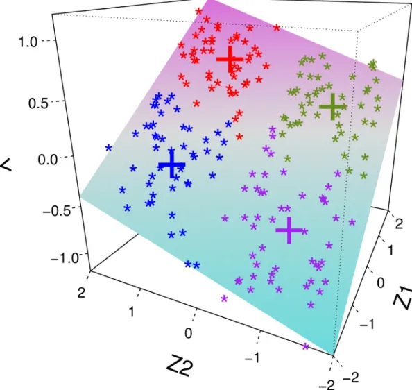
associ-ated with outcomes. InFig 2we present an example of one i.i.d. sample from (Y,Z1,Z2), where
we demonstrate four archetypal clusters associated with different response outcomes in different colors. This simulation setting illustrates a simple case where archetypes of functional patterns are associated with response.
Since we only have sparse and noisy longitudinal observationsX~½j�ofX[j]
, we first estimate
Eðξ½j�jX~½j�Þfor eachj-th trajectory marginally by applying FPCA based on the conditional
expectation technique (PACE) [41] toðX~½ij� : 1�i�nÞ. For computation, we used the
“fdapace” package in R [63], wheref^ξ½ij� ¼ ðx^ ½j� i1;x^ ½j� i2Þ > : 1�i�ngdenotes estimates of
Eðξ½ij�jX~i½j�Þ, 1�i�n, obtained from the PACE algorithm. Implementing the proposed method
described in the Methodology section, we obtain four clusters^Smbased on the (1−α)-HDR
method and standardized PC scores of multiple traits as inEq (7). We considered the
perfor-mance of our proposed methodology for the identification of risk clusters in comparison to
using the univariate traits separately. Similarly, we obtained the marginal four clusters^S½j�
m
based on the 95%-HDR method analogously to the above and standardized the individual FPC
scores of eachj-th trait as follows:
^ S½1j� ¼ f1�i�n: ^ξ ½j� i 2=R^ ½j�ð1 aÞ; j^x½j� i1j=ð^l ½j� 1Þ 1=2 >j^x½i2j�j=ðl^½2j�Þ 1=2 ; ^x½i1j�>0g; ^ S½2j� ¼ f1�i�n: ^ξ ½j� i 2=R^ ½j�ð1 aÞ; j^x½j� i1j=ð^l ½j� 1Þ 1=2 <j^x½i2j�j=ðl^½2j�Þ 1=2 ; ^x½i2j�>0g; ^ S½3j� ¼ f1�i�n: ^ξ ½j� i 2=R^ ½j� ð1 aÞ; j^xi1j=ð½j� ^l½1j�Þ 1=2 >j^x½i2j�j=ðl^ ½j� 2Þ 1=2 ; ^x½i1j�<0g; ^ S½4j� ¼ f1�i�n: ^ξ ½j� i 2=R^½j�ð1 aÞ; j^x ½j� i1j=ð^l½1j�Þ 1=2 <j^x½i2j�j=ðl^ ½j� 2Þ 1=2 ; ^x½i2j�<0g; ð10Þ whereR^½j�ð1 aÞis the (1−α)-HDR of^ξ½j� i .
We report the simulation results inTable 1, where the numbers of joint extreme trajectory clusters associated with outcomes obtained from 1000 Monte Carlo repetitions with sample
sizen= 1000 are shown forα= 0.05. Tukey’s post-hoc multiple comparison was employed to
determine how many associated clusters exist at each Monte Carlo run. That is, at each repeti-tion, we counted the subgroups which are completely separated by Tukey’s post-hoc analysis. By comparing conditional mean differences of outcomes between the four extreme clusters, we found that the proposed method identified more risk clusters than the marginal methods which detected two clusters on average for all cases. The joint method identified the three or
four of the archetype clusters which depict (highZ1, highZ2), (highZ1, lowZ2), (lowZ1, high
Z2) and (lowZ1, lowZ2) up to 90.4% (= 59.8% + 30.6%). This result supports the use of
multi-ple trajectories instead of a single trajectory when identifying archetypes of risk sets. This applies even as the first two PC scores have less than 50% FVE, as in this simulation example. Fig 2. Example for visualization of observations from simulation. The proposed method identifies clusters associated with
response outcomesYcharacterized by archetypal covariate levels Z = (Z1,Z2), for example (highZ1, highZ2), (highZ1, lowZ2),
(lowZ1, highZ2) and (lowZ1, lowZ2), which are symbolized by red, purple, green and blue points, respectively, where the
crosses denote the cluster centers. The surface demonstrates the conditional mean response when regressingYon Z = (Z1,Z2)
forn= 200 data points.
Analysis of PROBIT data
Marginal analysis for longitudinal measurements of growth traits. PROBIT contains three main time-varying traits; head circumference (HC), body length (LN) and weight (WT). For the marginal FPCA of these three variables, we applied the PACE technique introduced in the Methodology section, since we only have sparse and irregular observations available. As in
the simulation study, we also used the “fdapace” package in R [63]. Auto-covariance
func-tions of each time-varying trait were reconstructed by the first two eigenfuncfunc-tions. The frac-tions of variance explained (FVEs) were 97.70%, 96.92% and 98.14% for HC, LN and WT,
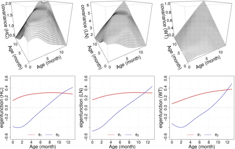
respectively. SeeFig 3for illustrations of estimated auto-covariance functions and
eigenfunc-tions. The first and second eigenfunctions can be regarded as “General growth” and “Growth acceleration”, respectively. Based on the observed high FVE coverages, we assume in the rest of the paper that these two qualitative features carry information about the longitudinal pat-terns of time-varying growth traits in the PROBIT data.
The marginal analysis of outlying subgroups was performed with a (1−α)-high density
region (HDR) withα= 0.05. Subjects were classified as “normal” if they belonged to the 95%
support region in the HDR criterion as inEq (4), while outlying subjects were classified as 5%
extreme cases falling outside the HDR criterion. In this study, we considered four exclusive
subgroups as inEq (10), where the trait index [j], 1�j�3, stands for HC, LN and WT,
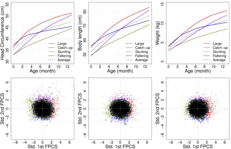
respectively. The four outlying subgroups correspond to distinctive growth patterns, which can be labeled as “Generally Large”, “Catch-up”, “Stunting” and “Faltering” (Fig 4). We found that the outlying patterns were discordant across traits. For example, subjects who were classi-fied into the generally large head circumference subgroup could be normal for body length or
weight, and vice versa. Moreover, as there are 43-combinations of subgroups entailed by the
marginal analysis, it is difficult to associate all these multiple trajectory patterns with the response of interest, which is IQ at 6.5 years.
Potential risk subgroups for cognitive development. We constructed joint outlying sub-groups of multiple time-varying traits based on the HDR method and standardized PC scores
of multiple traitsð^z½ij� ¼x^ ½j� ik=ðl^ ½j� kÞ 1=2 : 1�k�2;1�j�3Þas described inEq (7). Principal
component analysis results for the six FPC scores are presented inTable 2, where the first and
second FPC stand for scores of general growth and growth acceleration, respectively. We found that these two features were captured in the first two PC loadings. In this study, we Table 1. Simulation results for identification of at-risk multiple trajectories clusters associated with response outcomes.
Number of risk clusters associated with outcomes
Marginal method Joint method
PC-FPC j= 1 j= 2 j= 3 <2 3.6% 5.0% 4.7% 0.0% 2 62.3% 83.0% 84.0% 9.6% 3 31.7% 11.5% 10.8% 59.8% 4 2.4% 0.5% 0.5% 30.6%
For 1000 Monte Carlo (MC) repetitions with sample sizen= 1000, the numbers of risk clusters were identified by analysis of variance (ANOVA) and Tukey’s multiple comparisons with a family-wise significance level 0.05. At each repetition, we counted subgroups completely separated by Tukey’s post-hoc analysis. For example, we identify two clusters if all subgroups included in a cluster show significant differences in pairwise comparison (family-wise significance level 0.05) against the other cluster members. Percentages in each column of the table demonstrate how many clusters are detected through 1000 MC repetitions. For the comparison with the marginal method, we applied the same procedure, using the marginal trajectory information only forj= 1, 2, 3, respectively.
focus on the first two PC scores as they explain more than 95% of the variation for each of the
three modalities [41,42,45].
On the other hand, socio-economic factors affect childhood intelligence in ways that are
not reflected in the FPCA of time-varying traits [26,27]. To avoid confounding effects by
socio-economic variables, we used a linear mixed effects model to reduce the influence of the socio-economic indicators. Hospital information was treated as a random effect as it is related to the random clustered design of the PROBIT study. We used the residuals of the lin-ear mixed effects model and marginalized the effect of the potentially confounding variables considered above. For details of the data preprocessing, we refer to [22] and [13].
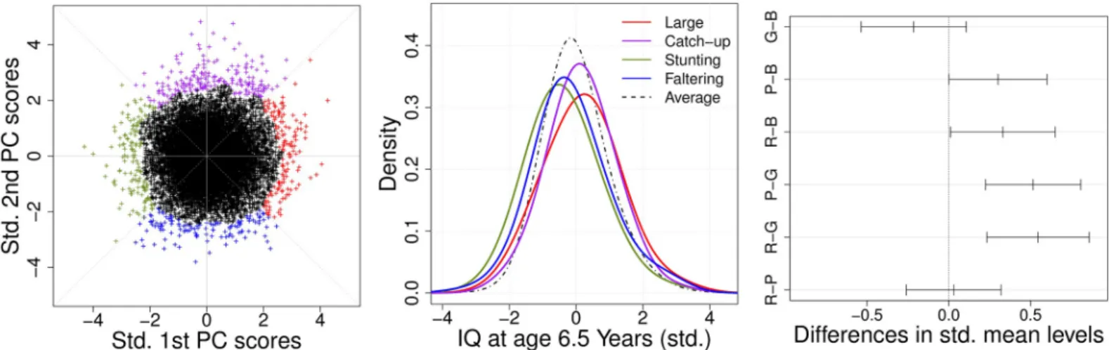
InFig 5, we find that conditional densities of IQ measured at 6.5 years, given the joint outly-ing subgroups, exhibited different distributional behaviors. The four subgroups were con-structed by a principal component analysis of the standardized six FPC scores for HC, LN and WT. The significance of the group mean differences was examined by one-way ANOVA (p-value = 0.002), and also by the Kruskal-Wallis rank sum test [62], a nonparametric procedure
for one-way ANOVA (p-value<0.001), so that the results were qualitatively the same. For a
more detailed comparison, we performed post-hoc analysis with Tukey’s multiple comparison
procedure. As shown inTable 3andFig 5, we found significant mean differences among
Fig 3. Estimated auto-covariance functions and eigenfunctions. Estimated auto-covariance functionsG(s,t) (top) and the corresponding first two eigenfunctions
ϕ1(t) andϕ2(t) (bottom) as inEq (3)for head circumference (HC, left), body length (LN, middle) and weight (WT, right), respectively. Eigenfunctions represent the
qualitative factors “General growth” (red) and “Growth acceleration” (blue). The cumulative fractions of variation explained (FVE) of the first two components are 97.70%, 96.92% and 98.14% for HC, LN and WT, respectively.
Fig 4. Extreme functional patterns from marginal analysis. Head circumference (HC, left), body length (LN, middle) and weight (WT, right) traits, respectively.
Four outlying clusters (falling into the smallest 5% of the bivariate density) are demonstrated with respective different colors, with estimated mean curves corresponding to the four outlying subgroups, respectively, which represent the four qualitative longitudinal growth patterns: “Generally Large” (red), “Catch-up” (purple), “Stunting” (green) and “Faltering” (blue) (top panels). The corresponding scatterplots for the first two functional principal component scores (bottom).
https://doi.org/10.1371/journal.pone.0207073.g004
Table 2. Principal component analysis of functional principal components. qualitative feature of joint FPCs marginal FPC factor PC loadings PC1 PC2 PC3 PC4 PC5 PC6 General growth HC-FPC1 0.502 0.155 0.457 0.690 0.044 0.191 LN-FPC1 0.552 0.198 -0.289 -0.430 0.243 0.574 WT-FPC1 0.527 0.331 -0.109 -0.182 -0.383 -0.649 Growth acceleration HC-FPC2 -0.216 0.517 0.688 -0.422 0.188 -0.020 LN-FPC2 -0.185 0.546 -0.432 0.324 0.570 -0.227 WT-FPC2 -0.291 0.512 -0.190 0.154 -0.657 0.402 partial FVE 0.382 0.261 0.122 0.094 0.088 0.053 cumulative FVE 0.382 0.643 0.765 0.859 0.947 1.000
Principal component analysis for the variance-covariance matrix of the first two marginal functional principal component scores (FPCs) for head circumference (HC), body length (LN) and weight (WT).
outlying subgroups in a family-wise 5%-level test. “Stunting” and “Faltering” were associated with higher risk in comparison with the “Generally Large” and “Catch-up” subgroups. Similar results were obtained by using the nonparametric procedure for pairwise comparisons of the Tukey-Kramer test. We also applied several multiple comparison techniques such as Bonfer-roni and Benjamini-Hochberg methods for post-hoc analysis and similar results were obtained by controlling false discovery rate (FDR) at 5%. For example, we found that “Stunting” and “Faltering” were associated with higher risk in comparison with the “Generally Large” and “Catch-up” subgroups after application of both procedures. The results were suggestive of higher risk for “Faltering” versus “Catch-up” (p-value = 0.060 after Bonferroni correction).
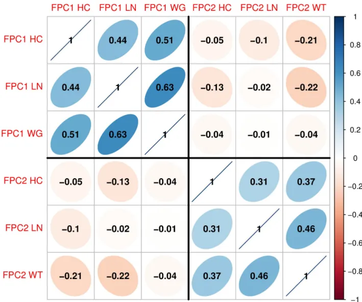
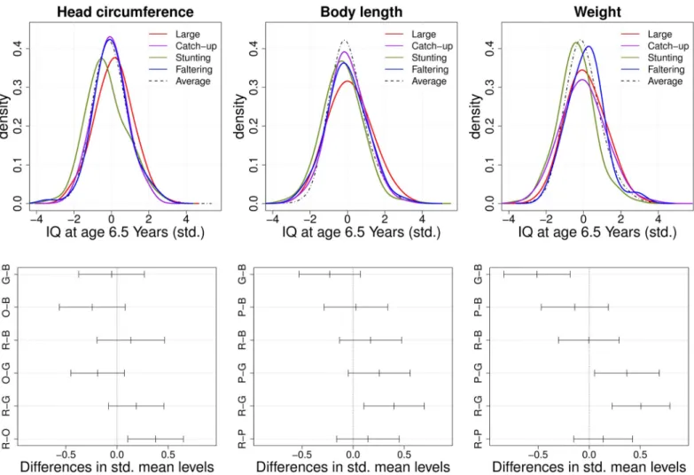
We close this section with a short remark on Figs6and7which presents the result of the
marginal analysis as described in the Simulation study section. In contrast to the proposed joint method, we found that the marginal procedures may not effectively detect risk growth patterns associated with long-term IQ outcomes. From the post-hoc analysis, “Generally Large” and “Stunting” subgroups had significantly different IQ performance for head
circum-ference (p-value = 0.002), body length (p-value = 0.003) and weight (p-value<0.001), but no
significant difference was found between other subgroups such as “Catch-up” or “Faltering” for head circumference and body length. We note that “Stunting” for one of the marginal com-ponents may not be an at-risk growth pattern associated with IQ development compared to Fig 5. Extreme subgroup identification from the proposed method. (Left panel) Scatterplot of 95% high density region clustering from principal component analysis
for head circumference, body length and weight and (Middle panel) the corresponding conditional kernel density estimates for long-term intelligence for each subgroup. Here, qualitative growth patterns include “Generally Large” (red), “Catch-up” (purple), “Stunting” (green) and “Faltering” (blue), whereas the black dashed line represents the “normal” subgroup that consists of subjects who do not belong to the four outlying subgroups. (Right panel) Tukey’s multiple comparisons of mean differences for standardized IQ along outlying subgroups are demonstrated by family-wise 95% confidence intervals, where we label the four subgroups as R (red, “Generally Large”), P (purple, “Catch-up”), G (green, “Stunting”) and B (blue, “Faltering”).
https://doi.org/10.1371/journal.pone.0207073.g005
Table 3. One-way ANOVA for subgroup detection.
variation df sum of sq. mean sq.
subgroup 3 27.002 9.001
residuals 598 631.902 1.057
total 601 658.904
F-value = 8.518 p-value<0.001
One-way ANOVA result provides evidence for differences in group means of long-term IQ for the four outlying subgroups “Generally Large”, “Catch-up”, “Stunting” and “Faltering”.
the other subgroups. Moreover, “Faltering” for weight showed higher IQ performances than
the “Stunting” subgroup (p-values<0.001), while failure to thrive in infancy, defined as
weight faltering in the first 9 months of life, was previously found to be associated with persis-tent deficits in intellectual development when measured at 8 years [64]. These results suggest that the combination of multiple growth patterns can indeed be beneficial for identifying risk subgroups associated with IQ outcomes.
Discussion
This paper outlines a statistical framework for exploring multivariate functional patterns deduced from sparsely and irregularly sampled longitudinal data and their association with long-term outcomes. For the joint analysis of children’s growth and IQ in the PROBIT data, we propose a straightforward way to combine multiple growth indicators under a single frame-work. We extract multiple growth features jointly, by using standard multivariate analysis of Fig 6. Correlation plot. Correlations between the first two functional principal component (FPC) scores of head circumference (HC), body length
(LN) and weight (WT). FPC scores among the first and second components have positive correlations, respectively, which suggests to combine the three growth features linearly with PC loadings as inTable 2.
the functional principal components. The major modes of growth variation are then repre-sented at the subject level and we can thus profile outlying multiple growth patterns, which can be considered as archetypes of growth.
The focus of this paper is how to combine multivariate functional data to identify extremal curve patterns and associate these features with responses. One may consider an alternative
application of multivariate functional principal component analysis as in [58,59,65,66] or
functional ANOVA [67–69] as alternatives. However, for all approaches it is critical how to determine outlying and extremal patterns jointly from multiple functional data, and the high-density region (HDR) method to detect outlying functional principal components that we adopt here is a natural extension of similar nonparametric approaches in multivariate data analysis. Recently several related studies have been introduced for functional outlier detection [54,70,71] but it still remains an open problem how to combine these with other methodolo-gies such as clustering and archetypal analysis.
In the PROBIT growth data analysis, we identified four archetypal subgroups of infant growth patterns, namely “Stunting”, “Faltering”, “Generally Large” and “Catch-up”. In addi-tion we also found that covariance structures have marginally similar patterns across the Fig 7. Marginal subgroup identification. (Top panels) Conditional kernel density estimators and (bottom panels) illustrations of Tukey’s multiple comparisons for
standardized IQ along outlying subgroups. As inFig 5, the first two functional principal component (FPC) scores are used to construct subgroups for head circumference (left), body length (middle) and weight (right), labeled R (red, “Generally Large”), P (purple, “Catch-up”), G (green, “Stunting”) and B (blue, “Faltering”).
functional traits considered; head-circumference, body length and weight. According to our analysis, subgroups corresponding to “Stunting” and “Faltering” in the infant period had lower downstream IQ compared to “Generally Large” and “Catch-up” subgroups. This finding is supported by previous studies that link deficient infant growth and later life cognitive perfor-mance degradation.
It is worth mentioning that single growth indicators were not found to be associated with risk of lowered IQ, and the marginal analysis of single growth traits did not produce
informa-tive results in the PROBIT analysis (SeeFig 7). Also, there is a possibility that the absence of
any measure of cognitive ability during infancy in the data could be explained by reverse cau-sality, namely, poor cognitive function in infancy may have led to worse dietary intake. Both may have been consequences of poor parenting or unmeasured insults during pregnancy or infancy. The proposed methods are not limited to specific data structures, such as growth data, but can be applied to many other kinds of longitudinal data as well, whenever a downstream outcome is of interest.
Acknowledgments
This study was supported by the Bill & Melinda Gates Foundation (OPP1119700). The article contents are the sole responsibility of the authors and may not necessarily represent the official views of the Bill & Melinda Gates Foundation or other agencies that may have supported the primary data studies used in the present study.
Author Contributions
Conceptualization: Hans-Georg Mu¨ller.
Data curation: Michael S. Kramer, Seungmi Yang. Formal analysis: Kyunghee Han.
Methodology: Kyunghee Han.
Project administration: Hans-Georg Mu¨ller.
Software: Kyunghee Han, Pantelis Z. Hadjipantelis. Supervision: Hans-Georg Mu¨ller.
Validation: Kyunghee Han, Pantelis Z. Hadjipantelis. Visualization: Kyunghee Han.
Writing – original draft: Kyunghee Han.
Writing – review & editing: Pantelis Z. Hadjipantelis, Jane-Ling Wang, Michael S. Kramer,
Seungmi Yang, Richard M. Martin, Hans-Georg Mu¨ller.
References
1. Shenkin SD, Starr JM, Deary IJ. Birth weight and cognitive ability in childhood: A systematic review. Psychological Bulletin. 2004; 130(6):989.https://doi.org/10.1037/0033-2909.130.6.989PMID:
15535745
2. Morley R, Fewtrell MS, Abbott RA, Stephenson T, MacFadyen U, Lucas A. Neurodevelopment in chil-dren born small for gestational age: A randomized trial of nutrient-enriched versus standard formula and comparison with a reference breastfed group. Pediatrics. 2004; 113(3):515–521.https://doi.org/10. 1542/peds.113.3.515PMID:14993543
3. Ra¨ikko¨nen K, Forse´ n T, Henriksson M, Kajantie E, Heinonen K, Pesonen AK, et al. Growth Trajectories and Intellectual Abilities in Young Adulthood: The Helsinki Birth Cohort Study. American Journal of Epi-demiology. 2009; 170(4):447–455.https://doi.org/10.1093/aje/kwp132PMID:19528290
4. Yang S, Tilling K, Martin R, Davies N, Ben-Shlomo Y, Kramer MS. Pre-natal and post-natal growth tra-jectories and childhood cognitive ability and mental health. International Journal of Epidemiology. 2011; 40(5):1215–1226.https://doi.org/10.1093/ije/dyr094PMID:21764769
5. Sudfeld CR, McCoy DC, Danaei G, Fink G, Ezzati M, Andrews KG, et al. Linear growth and child devel-opment in low-and middle-income countries: a meta-analysis. Pediatrics. 2015; 135(5):e1266–e1275.
https://doi.org/10.1542/peds.2014-3111PMID:25847806
6. Crookston BT, Schott W, Cueto S, Dearden KA, Engle P, Georgiadis A, et al. Postinfancy growth, schooling, and cognitive achievement: Young Lives. The American Journal of Clinical Nutrition. 2013; 98(6):1555–1563.https://doi.org/10.3945/ajcn.113.067561PMID:24067665
7. Lundeen EA, Behrman JR, Crookston BT, Dearden KA, Engle P, Georgiadis A, et al. Growth faltering and recovery in children aged 1-8 years in four low- and middle-income countries: Young Lives. Public Health Nutrition. 2014; 17(9):2131–2137.https://doi.org/10.1017/S1368980013003017PMID:24477079
8. Reid BM, Miller BS, Dorn LD, Desjardins C, Donzella B, Gunnar M. Early growth faltering in post-institu-tionalized youth and later anthropometric and pubertal development. Pediatric Research. 2017; 82 (2):278–284.https://doi.org/10.1038/pr.2017.35PMID:28170387
9. Keusch GT, Rosenberg IH, Denno DM, Duggan C, Guerrant RL, Lavery JV, et al. Implications of acquired environmental enteric dysfunction for growth and stunting in infants and children living in low-and middle-income countries. Food low-and Nutrition Bulletin. 2013; 34(3):357–364.https://doi.org/10. 1177/156482651303400308PMID:24167916
10. Gale CR, O’Callaghan FJ, Bredow M, Martyn CN, Avon Longitudinal Study of Parents and Children Study Team. The influence of head growth in fetal life, infancy, and childhood on intelligence at the ages of 4 and 8 years. Pediatrics. 2006; 118(4):1486–1492.https://doi.org/10.1542/peds.2005-2629PMID:
17015539
11. Lingam R, Hunt L, Golding J, Jongmans M, Emond A. Prevalence of developmental coordination disor-der using the DSM-IV at 7 years of age: A UK population–based study. Pediatrics. 2009; 123(4):e693– e700.https://doi.org/10.1542/peds.2008-1770PMID:19336359
12. Britto PR, Lye SJ, Proulx K, Yousafzai AK, Matthews SG, Vaivada T, et al. Nurturing care: Promoting early childhood development. The Lancet. 2017; 389(10064):7–13.https://doi.org/10.1016/S0140-6736 (16)31390-3
13. Hadjipantelis PZ, Han K, Wang JL, Yang S, Martin RM, Kramer MS, et al. Associating Growth in Infancy and Cognitive Performance in Early Childhood: A functional data analysis approach. ArXiv e-prints. 2018; 1808.01384.
14. Hall P,F, Mu¨ller HG, Wang JL. Properties of principal component methods for functional and longitudinal data analysis. Annals of Statistics. 2006; 34(3):1493–1517.https://doi.org/10.1214/
009053606000000272
15. Wang JL, Chiou J, Mu¨ller HG. Functional Data Analysis. Annual Review of Statistics and Its Application. 2016; 3:257–295.https://doi.org/10.1146/annurev-statistics-041715-033624
16. Wei Y. An approach to multivariate covariate-dependent quantile contours with application to bivariate conditional growth charts. Journal of the American Statistical Association. 2008; 103(481):397–409.
https://doi.org/10.1198/016214507000001472
17. Zhang W, Wei Y. Regression based principal component analysis for sparse functional data with appli-cations to screening growth paths. The Annals of Applied Statistics. 2015; 9(2):597–620.https://doi.org/ 10.1214/15-AOAS811
18. Park J, Ahn J. Clustering multivariate functional data with phase variation. Biometrics. 2017; 73(1):324– 333.https://doi.org/10.1111/biom.12546PMID:27218696
19. Cutler A, Breiman L. Archetypal analysis. Technometrics. 1994; 36(4):338–347.https://doi.org/10. 1080/00401706.1994.10485840
20. Vinue´ G, Epifanio I, Alemany S. Archetypoids: A new approach to define representative archetypal data. Computational Statistics & Data Analysis. 2015; 87:102–2015.https://doi.org/10.1016/j.csda. 2015.01.018
21. Epifanio I. Functional archetype and archetypoid analysis. Computational Statistics & Data Analysis. 2016; 104:24–34.https://doi.org/10.1016/j.csda.2016.06.007
22. Kramer MS, Chalmers B, Hodnett ED, Sevkovskaya Z, Dzikovich I, Shapiro S, et al. Promotion of Breastfeeding Intervention Trial (PROBIT): a randomized trial in the Republic of Belarus. Journal of the American Medical Association. 2001; 285(4):413–420.https://doi.org/10.1001/jama.285.4.413PMID:
11242425
23. Kramer MS, Kakuma R. The optimal duration of exclusive breastfeeding. In: Pickering LK, Morrow AL, Ruiz-Palacios GM, Schanler R, editors. Protecting Infants through Human Milk. Springer; 2004. p. 63– 77.
24. Tong S, McMichael AJ, Baghurst PA. Interactions between environmental lead exposure and sociode-mographic factors on cognitive development. Archives of Environmental Health. 2000; 55:330–335.
https://doi.org/10.1080/00039890009604025PMID:11063408
25. Walker SP, Wachs TD, Gardner JM, Lozoff B, Wasserman GA, Pollitt E, et al. Child development: Risk factors for adverse outcomes in developing countries. The Lancet. 2007; 369(9556):145–157.https:// doi.org/10.1016/S0140-6736(07)60076-2
26. Nisbett RE, Aronson J, Blair C, Dickens W, Flynn J, Halpern DF, et al. Intelligence: New findings and theoretical developments. American Psychologist. 2012; 67(2):130.https://doi.org/10.1037/a0026699
PMID:22233090
27. Smithers LG, Lynch JW, Yang S, Dahhou M, Kramer MS. Impact of neonatal growth on IQ and behavior at early school age. Pediatrics. 2013; 132(1):e53–e60.https://doi.org/10.1542/peds.2012-3497PMID:
23776123
28. Karhunen K. Zur Spektraltheorie Stochastischer Prozesse. Annales Academiae Scientiarum Fennicae Series A I, Mathematica. 1946; 7.
29. Loève M. Fonctions ale´atoiresàde´composition orthogonale exponentielle. La Revue Scientique. 1946; 84:159–162.
30. Ramsay J, Silverman BW. Functional data analysis. 2nd ed. Springer-Verlag, New York; 2005. 31. Dauxois J, Pousse A, Romain Y. Asymptotic theory for the principal component analysis of a vector
ran-dom function: Some applications to statistical inference. Journal of Multivariate Analysis. 1982; 12:136– 154.https://doi.org/10.1016/0047-259X(82)90088-4
32. Besse P, Ramsay JO. Principal components analysis of sampled functions. Psychometrika. 1986; 51:285–311.https://doi.org/10.1007/BF02293986
33. Silverman BW. Smoothed functional principal components analysis by choice of norm. Annals of Statis-tics. 1996; 24:1–24.https://doi.org/10.1214/aos/1033066196
34. Boente G, Fraiman R. Kernel-based functional principal components. Statistics & Probability Letters. 2000; 48:335–345.https://doi.org/10.1016/S0167-7152(00)00014-6
35. Hall P, Hosseini-Nasab M. On properties of functional principal components analysis. Journal of the Royal Statistical Society: Series B. 2006; 68:109–126.https://doi.org/10.1111/j.1467-9868.2005.00535.x
36. Li Y, Wang N, Carroll RJ. Selecting the number of principal components in functional data. Journal of the American Statistical Association. 2013; 108:1284–1291.https://doi.org/10.1080/01621459.2013. 788980
37. James G, Hastie T, Sugar C. Principal component models for sparse functional data. Biometrika. 2000; 87:587–602.https://doi.org/10.1093/biomet/87.3.587
38. Rice JA, Wu CO. Nonparametric mixed effects models for unequally sampled noisy curves. Biometrika. 2001; 57:253–259.https://doi.org/10.1111/j.0006-341X.2001.00253.x
39. Mu¨ller HG. Functional modeling and classification of longitudinal data. Scandinavian Journal of Statis-tics. 2005; 32(2):223–240.https://doi.org/10.1111/j.1467-9469.2005.00429.x
40. Yao F, Lee T. Penalized spline models for functional principal component analysis. Journal of the Royal Statistical Society: Series B. 2006; 68:3–25.https://doi.org/10.1111/j.1467-9868.2005.00530.x
41. Yao F, Mu¨ller HG, Wang JL. Functional data analysis for sparse longitudinal data. Journal of the Ameri-can Statistical Association. 2005; 100(470):577–590.https://doi.org/10.1198/016214504000001745
42. Yao F, Mu¨ller HG, Wang JL. Functional linear regression analysis for longitudinal data. Annals of Statis-tics. 2005; 33(6):2873–2903.https://doi.org/10.1214/009053605000000660
43. Mu¨ller HG. Functional modeling of longitudinal data. In: Fitzmaurice G, Davidian M, Verbeke G, Molen-berghs G, editors. Longitudinal Data Analysis. CRC Press; 2009. p. 233–252.
44. Jones MC, Rice JA. Displaying the important features of large collections of similar curves. The Ameri-can Statistician. 1992; 46(2):140–145.https://doi.org/10.2307/2684184
45. Leng X, Mu¨ller HG. Classification using functional data analysis for temporal gene expression data. Bio-informatics. 2006; 22(1):68–76.https://doi.org/10.1093/bioinformatics/bti742PMID:16257986
46. Rousseeuw PJ, Ruts I, Tukey JW. The bagplot: A bivariate boxplot. The American Statistician. 1999; 53 (4):382–387.https://doi.org/10.2307/2686061
47. Tukey JW. Mathematics and the picturing of data. In: James RD, editor. Proceedings of the International Congress of Mathematicians. vol. 2. Canadian Mathematical Society; 1975. p. 523–531.
48. Zuo Y. Projection-based depth functions and associated medians. Annals of Statistics. 2003; 31:1460– 1490.https://doi.org/10.1214/aos/1065705115
49. Agostinelli C, Romanazzi M. Local depth. Journal of Statistical Planning and Inference. 2011; 141 (2):817–830.https://doi.org/10.1016/j.jspi.2010.08.001
50. Hyndman RJ. Computing and graphing highest density regions. The American Statistician. 1996; 50 (2):241–250.https://doi.org/10.2307/2684423
51. Scott DW. Multivariate density estimation: Theory, practice and visualization. 2nd ed. Wiley, New York; 2015.
52. Hyndman RJ, Shang HL. Rainbow plots, bagplots and boxplots for functional data. Journal of Computa-tional and Graphical Statistics. 2010; 19:29–45.https://doi.org/10.1198/jcgs.2009.08158
53. Sun Y, Genton MG. Functional boxplots. Journal of Computational and Graphical Statistics. 2011; 20 (2):316–334.https://doi.org/10.1198/jcgs.2011.09224
54. Hubert M, Rousseeuw PJ, Segaert P. Multivariate functional outlier detection. Statistical Methods & Applications. 2015; 24(2):177–202.https://doi.org/10.1007/s10260-015-0297-8
55. Narisetty NN, Nair VN. Extremal depth for functional data and applications. Journal of the American Sta-tistical Association. 2016; 111(516):1705–1714.https://doi.org/10.1080/01621459.2015.1110033
56. Zhou L, Huang JZ, Carroll RJ. Joint modeling of paired sparse functional data using principal compo-nents. Biometrika. 2008; 95(3):601–619.https://doi.org/10.1093/biomet/asn035PMID:19396364
57. Chiou JM, Mu¨ller HG. Linear manifold modeling of multivariate functional data. Journal of the Royal Sta-tistical Society: Series B. 2011; 76(3):605–626.https://doi.org/10.1111/rssb.12038
58. Chiou JM, Chen YT, Yang YF. Multivariate functional principal component analysis: A normalization approach. Statistica Sinica. 2014; 24:1571–1596.
59. Happ C, Greven S. Multivariate functional principal component analysis for data observed on different (dimensional) domains. Journal of the American Statistical Association. 2018; 113(522):649–659.
https://doi.org/10.1080/01621459.2016.1273115
60. Benjamini Y, Hochberg Y. Controlling the false discovery rate: a practical and powerful approach to mul-tiple testing. Journal of the Royal Statistical Society Series B (Methodological). 1995; p. 289–300. 61. Tukey JW. Comparing individual means in the analysis of variance. Biometrika. 1949; 5(2):99–114.
https://doi.org/10.2307/3001913
62. Kruskal WH, Wallis WA. Use of ranks in one-criterion variance analysis. Journal of the American Statis-tical Association. 1952; 47(260):583–621.https://doi.org/10.1080/01621459.1952.10483441
63. fdapace. R Package: Functional Data Analysis and Empirical Dynamics; version 0.4.0. Available from:https://CRAN.R-project.org/package=fdapace.
64. Emond AM, Blair PS, Emmett PM, Drewett RF. Weight faltering in infancy and IQ levels at 8 years in the Avon Longitudinal Study of Parents and Children. Pediatrics. 2007; 120(4):e1051–e1058.https://doi. org/10.1542/peds.2006-2295PMID:17908725
65. Berrendero JR, Justel A, Svarc M. Principal components for multivariate functional data. Computational Statistics & Data Analysis. 2011; 55(9):2619–2634.https://doi.org/10.1016/j.csda.2011.03.011
66. Go´recki T, Krzyśko M, Waszak Ł, Wołyński W. Selected statistical methods of data analysis for multi-variate functional data. Statistical Papers. 2018; 59(1):153–182. https://doi.org/10.1007/s00362-016-0757-8
67. Cuevas A, Febrero M, Fraiman R. An anova test for functional data. Computational Statistics & Data Analysis. 2004; 47(1):111–122.https://doi.org/10.1016/j.csda.2003.10.021
68. Go´recki T, Smaga Ł. Multivariate analysis of variance for functional data. Journal of Applied Statistics. 2017; 44(12):2172–2189.https://doi.org/10.1080/02664763.2016.1247791
69. Zhang JT. Analysis of variance for functional data. Chapman and Hall/CRC; 2013.
70. Sawant P, Billor N, Shin H. Functional outlier detection with robust functional principal component analy-sis. Computational Statistics. 2012; 27(1):83–102.https://doi.org/10.1007/s00180-011-0239-3
71. Febrero M, Galeano P, Gonza´lez-Manteiga W. Outlier detection in functional data by depth measures, with application to identify abnormal NOx levels. Environmetrics: The official journal of the International Environmetrics Society. 2008; 19(4):331–345.https://doi.org/10.1002/env.878