Analysis and Control of Power System with Wind Generation

(1)

Analysis and Control of Power System

with Wind Generation

Linash Puthenpurayil Kunjumuhammed

Thesis submitted for the degree of

Doctor of Philosophy

Imperial College London

Department of Electrical and Electronic Engineering Control and Power Research Group

(2)

Abstract

The objective of this work is to study the impact of large scale wind integration in the dynamic performance of power system. The variable nature of wind generation has been driving power system operating conditions from a largely predictable one to highly variable and stochastic. Such changes will have huge impact in the dynamic performance of the system.

The limitation in dynamic performance is one of the constraints for effective utilization of available transmission and generation resources. The thesis draws a qualitative behavior of inter-area mode damping with increased wind penetration. The factors such as changes in power flow and displacement of conventional generators, resulting from large scale integration of wind are considered. Another consequence of wind variability is the changes in controllability and observability in the context of power system damping control when operating conditions vary significantly. The modal controllability and observability decide the controller performance, large variation of which can result in inefficient control effort and poor stability margin. A controller design methodology using robust signal selection is presented for power systems with increased variability in operating conditions. The core of this method is based on stochastic error co-variance matrix of modal residue due to large variation in operating condition. The work further explores possibility of using wind farms for damping control using active and reactive power modulation. Interaction of damping controller with torsional mode of wind turbines is analyzed and a signal selection criteria is presented to reduce the interaction. Also, selection of active or reactive power modulation of wind farm for damping control is discussed. The outcome of this research offers deeper insight into the power system dynamic problem in the presence of large asynchronous generation such as wind.

(3)

Dedicated to

(4)

Acknowledgements

I would like to express my sincere gratitude to my supervisor Dr. Bikash Pal for his continuous support and guidance through all stages of my research. He supported me throughout my thesis with patience and knowledge whilst allowing me the room to work in my own way.

I extend my thanks to Dr. Ravindra Singh for his inspiring discussions and valuable suggestions during this research work. A special thanks to Dr. Krishna Anaparthi for supporting me during my Secondment in GE global Research. I would also like to thank all the members of the control and power research group for providing an enjoyable working environment.

I would also like to acknowledge the financial support provided by EPSRC, UK under Flexnet project and the European Union under FP7 Real Smart project.

Outside office, I have been blessed with friendly and cheerful friends, and I am indebted to each of them for all their help and support. I am especially grateful to Najeem and Reeja for their timely help making my stay in London a lot easier.

I am thankful to my wife, Ancy, and my son, Layan, for their unconditional love, support and patience. Their sacrifice for this work has been invaluable. Above all, my parents and other family members receive my deepest gratitude for their dedication, love and support, which go beyond words.

(5)

Declaration

I hereby declare that the work presented in this thesis is my own work, and, wherever appropriate, contributions from other people have been acknowledged.

Linash Puthenpurayil Kunjumuhammed 13 September 2012, London

(6)

List of Figures

2.1 Generation despatch in WestConnect study area in April 2006 . . . . 36

2.2 Effect of wind penetration in West Denmark Grid during 10 to 16 January 2005 . . . 36

2.3 Effect of wind penetration on thermal generation scheduling in GB network . . . 38

2.4 Effect of wind penetration on operating Reserve Requirement in GB network for January 2020 . . . 39

3.1 Overview of power system simulation program . . . 42

3.2 Block diagram representation of synchronous machine model . . . 43

3.3 Block diagram representation of excitation system model . . . 45

3.4 Block diagram representation of turbine governor system model . . . 45

3.5 Various schematic representations of TCSC . . . 46

3.6 Small signal dynamic model of TCSC . . . 46

3.7 Small signal dynamic model of SVC . . . 47

3.8 Algebraic loop representation . . . 49

3.9 Four machine two-area test system . . . 52

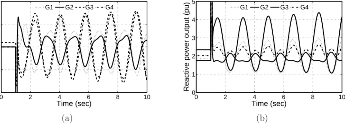
3.10 Four machine two-area test system time domain simulation results; generator active and reactive power outputs . . . 52

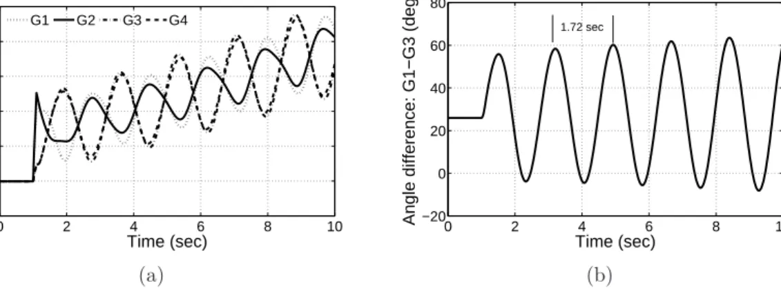
3.11 Four machine two-area test system time domain simulation results; Excitation system output and terminal voltage of synchronous generators 53 3.12 Four machine two-area test system time domain simulation results; Generator speeds, and angle difference between G1 and G3 . . . 53

3.13 Eigenvalues of four machine two-area test system with SVC . . . 56

3.14 Four machine two-area test system time domain simulation results with SVC based damping controller; Generator active power outputs . . . 56

3.15 Four machine two-area test system time domain simulation results with SVC based damping controller; Speed of generators . . . 57

(12)

3.16 Four machine two-area test system time domain simulation results with SVC based damping controller; SVC bus voltage, SVC susceptance,

and Angle difference between generators G1 and G3 . . . 57

4.1 Schematic diagram of Type-3 and Type-4 WTG systems . . . 60

4.2 Block diagram representation of wind turbine generator system . . . . 61

4.3 Single machine infinite bus test system . . . 62

4.4 Two-area system with wind farm . . . 63

4.5 Block diagram representation of Detailed WTG model . . . 63

4.6 Wind speed-power output curve of WTG system . . . 64

4.7 Pitch control and actuator model of WTG . . . 64

4.8 Schematic diagram of rotor side converter of WTG . . . 67

4.9 Simulation results of SMIB system using detailed WTG model: Response to step change to infinite bus voltage . . . 69

4.10 Simulation results of SMIB system using detailed WTG model: Response to step change to voltage reference input . . . 69

4.11 Simulation results of SMIB system using detailed WTG model: Response to a three phase fault at infinite bus . . . 70

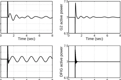
4.12 Response of two-area test system using detailed WTG model to a three phase fault: Active power output of generators . . . 71

4.13 Response of two-area test system using detailed WTG model to a three phase fault: Reactive power output of generators . . . 71

4.14 Response of two-area test system using detailed WTG model to a three phase fault: Angle difference between generators in different area . . . 72

4.15 Schematic representation of generic Type-3 WTG model . . . 74

4.16 Generator converter model of generic type-3 WTG model . . . 75

4.17 Reactive power control loop of generic type-3 WTG model . . . 75

4.18 Active power control loop of generic type-3 WTG model . . . 76

4.19 Pitch angle control loop of type-3 WTG model . . . 76

4.20 Turbine model of type-3 WTG model . . . 77

4.21 Simulation results of SMIB system using Type-3 WTG model: Re-sponse to step change in infinite bus voltage . . . 77

4.22 Simulation results of SMIB system using Type-3 WTG model: Re-sponse to step change in terminal voltage controller reference input . 78 4.23 Simulation results of SMIB system using Type-3 WTG model: Re-sponse to step a three phase fault at infinite bus . . . 78

(13)

4.25 Generator converter model of generic Type-4 WTG model . . . 79 4.26 Reactive power control loop of generic Type-4 WTG model . . . 80 4.27 Active power control loop of generic Type-4 WTG model . . . 80 4.28 Simulation results of SMIB system using Type-4 WTG model:

Re-sponse to a step change in infinite bus voltage and a step change in voltage controller reference input. . . 81 4.29 Response of two-area test system using generic Type-3 WTG model to

a three phase fault at bus #7 . . . 82 4.30 Magnified view of Fig. 4.29 showing response during fault . . . 82 5.1 Overview of two-area system with wind farm . . . 85 5.2 Inter-area mode shift for incremental change in wind penetration in

the two area test system . . . 89 5.3 Figure showing the impact of wind penetration on modal residue . . . 91 5.4 Representative GB system network . . . 94 5.5 Electromechanical modes of representative GB system for 2010

oper-ating scenario . . . 97 5.6 Response of GB system following a three phase bus fault for 100 msec 97 6.1 Damping line representing different damping ratios . . . 103 6.2 Schematic diagram of closed loop system . . . 104 6.3 Inter-area mode shift in a two-area system using SVC based damping

controller H(s) . . . 106 6.4 Inter-area mode shift in a two-area system using SVC based damping

controllerH′(s) . . . 107 6.5 Inter-area mode shift for a static gain controller (*) and modified

controller, H′(s) (o) for different feedback signals (a) P6−7, (b) P10−9,

(c) ωG1, and (d) ωG3 . . . 107

6.6 16 machine five area test system . . . 116 6.7 An example Weibull distribution and Wind speed vs power output

curve of WTG . . . 118 6.8 Histograms showing variation in generator output for different

operat-ing conditions of 16 machine test system . . . 120 6.9 Histograms showing variation in load for different operating conditions

(14)

6.10 Histogram showing variation in (a) total system load and (b) power transfer b/w area #1 & area #2 for different operating conditions of 16 machine test system . . . 121 6.11 Plot showing average value of bus voltage and generator power factor

for all operating conditions of sixteen machine test system . . . 122 6.12 Electromechanical modes of the sixteen machine system for all the

operating conditions . . . 123 6.13 Histogram showing variation in residue for nine feedback signals . . . 125 6.14 Error ellipse corresponding to various feedback signals of PSS . . . . 126 6.15 Eigenvalue shift with increase in PSS gain for an operating condition 127 6.16 Eigenvalues of the sixteen machine system with and without PSS for

all the operating conditions . . . 127 6.17 MISO controller structure . . . 128 6.18 Normalized average magnitude of residue of feedback signals

corre-sponding to IA1 . . . 128 6.19 Error ellipse of potential feedback signals passed criteria-1 to represent

IA1 . . . 130 6.20 Determinant of ECM of potential feedback signals passed criteria-1 to

represent IA1 . . . 130 6.21 Angle of residues for the signal I42−15 . . . 131

6.22 Angle of residues for the signal P61−30 . . . 132

6.23 Normalized average magnitude of residue for feedback signals corre-sponding to inter-area mode, IA2 . . . 133 6.24 Angle of residues for the signal P18−16 . . . 134

6.25 Bode plot of the TCSC damping controller . . . 137 6.26 Closed loop eigenvalues of the 16 machine system with damping

controllers . . . 137 7.1 Wind farm Power-Frequency Response Curve of Irish Grid . . . 141 7.2 Root locus plots showing effect of active power modulation on torsional

mode in two-area test system . . . 142 7.3 Normalized magnitude of residue corresponding to torsional mode for

active power reference input in the two-area test system with DFIG . 143 7.4 Plot showing eigenvalue shift for the two-area system with DFIG for

(15)

7.5 Closed loop response of two-area system with DFIG using damping controller modulating active power output: Plot shows angle difference between generators G1 and G3 . . . 144 7.6 Closed loop response of two-area system with DFIG using damping

controller modulating active power output: Plot shows active power output of DFIG . . . 145 7.7 Closed loop response of two-area system with DFIG using damping

controller modulating active power output: Plot shows reactive power output of DFIG . . . 145 7.8 Root locus plots showing effect of reactive power modulation on

torsional mode in two-area test system . . . 146 7.9 Closed loop response of two-area system with DFIG using damping

controller modulating reactive power output: Plot shows angle differ-ence between generators G1 and G3 . . . 147 7.10 Closed loop response of two-area system with DFIG using damping

controller modulating reactive power output: Plot shows active power output of DFIG . . . 147 7.11 Closed loop response of two-area system with DFIG using damping

controller modulating reactive power output: Plot shows reactive power output of DFIG . . . 148 7.12 Controllability of inter-area mode in representative GB system for

different wind farms under the nine operating conditions. . . 149 7.13 Average magnitude of residue for transfer function between different

feedback signals and voltage reference input of wind farm at bus #6; GB test system . . . 150 7.14 Eigenvalues of GB system with damping controller using reactive power

modulation . . . 151 7.15 Closed loop response of GB system using damping controller

modu-lating reactive power output: Plot shows angle difference between G1 and G23 . . . 151 7.16 Closed loop response of GB system using damping controller

modulat-ing reactive power output: Plot shows reactive power output of DFIG used for damping control . . . 151 7.17 Closed loop response of GB system using damping controller

modulat-ing reactive power output: Plot shows active power output of DFIG used for damping control . . . 152

(16)

7.18 Eigenvalues of GB system with damping controller using active power

modulation . . . 153

7.19 Closed loop response of GB system using damping controller modulat-ing active power output: Plot shows angle difference between G1 and G23 . . . 153

7.20 Closed loop response of GB system using damping controller modulat-ing active power output: Plot shows reactive power output of DFIG used for damping control . . . 153

7.21 Closed loop response of GB system using damping controller modu-lating active power output: Plot shows active power output of DFIG used for damping control . . . 154

A.1 Simulink representation of a first order transfer function . . . 159

A.2 Implementation of Torque-Angle loop . . . 160

A.3 Implementation of rotor electrical block shown in Fig. 3.2 . . . 161

G.1 Reactive power generation of different generators for the 2020 operating conditions of representative GB system . . . 190

G.2 Voltage profile of representative GB test system for the 2020 operating conditions . . . 191

(17)

List of Tables

3.1 Eigenvalues of the four machine two-area test system . . . 55

3.2 Mode shape of inter-area mode in two-area test system . . . 55

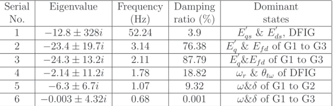
4.1 Complex eigenvalues of two-area test system with detailed WTG model 73 4.2 Complex eigenvalues of two-area test system with a Type-3 WTG . . 83

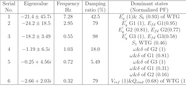
4.3 Complex eigenvalues of two-area test system with a Type-4 WTG . . 83

5.1 Impact of wind penetration on the stability of two-area test system; wind farm capacity equals one of the synchronous generators’ . . . 87

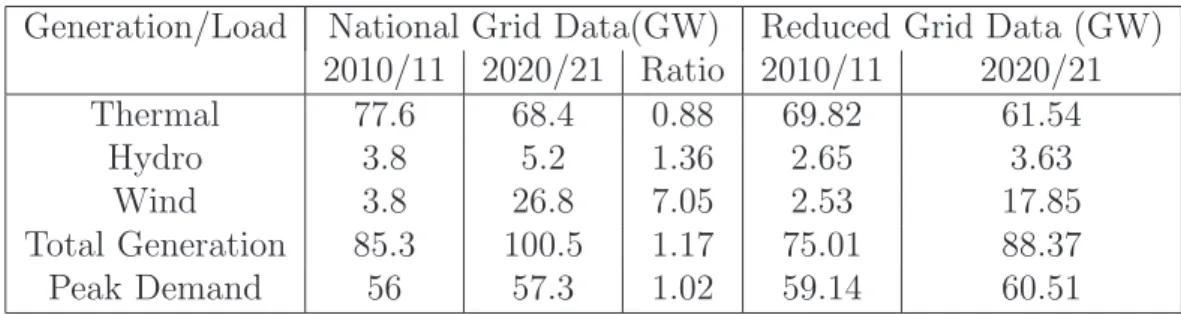
5.2 National grid forecast for GB electricity generation under “Gone Green”scenario . . . 92

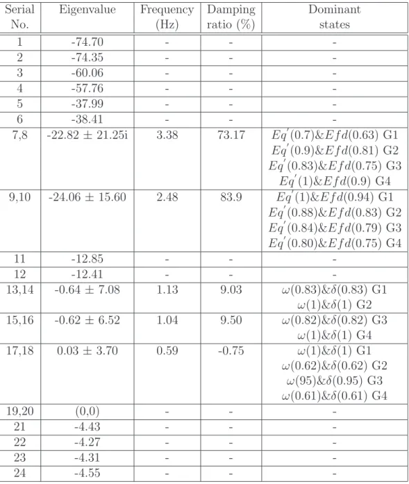
5.3 Change in generation across different group of generators in GB system 93 5.4 Electromechanical modes of representative GB system for 2010 oper-ating scenario . . . 96

5.5 Mode shape of the GB system inter-area mode . . . 96

5.6 Operating scenarios in representative GB network . . . 99

6.1 Residue and controller transfer function corresponding to different feedback signals for two-area test system using SVC based damping controller. . . 106

6.2 Modified controller transfer function for two-area test system using SVC based damping controller . . . 107

6.3 Criteria 3: influence of near by mode on signal selection . . . 114

6.4 Critical eigenvalue and dominant states of sixteen machine system . . 123

6.5 Characteristics of possible PSS feedback signals . . . 126

6.6 Potential feedback signals passed criteria-1 to represent IA1 . . . 129

6.7 Residue characteristics of signal I42−15 . . . 130

6.8 Residue characteristics of signal P61−30 . . . 132

6.9 Potential feedback signals passed Criteria-1 to represent IA2 . . . 133

(18)

6.11 Potential feedback signals passed Criteria-1 to represent IA3 . . . 135

6.12 Potential feedback signals passed criteria-1 to represent IA4 . . . 135

6.13 feedback signals for the TCSC damping controller . . . 135

B.1 Two area system: Bus data . . . 162

B.2 Two area system: Line data . . . 162

B.3 Two area system: Synchronous machine parameters . . . 163

B.4 Two area system: Excitation system data . . . 163

C.1 16 machine system: Bus data . . . 164

C.2 16 machine system: Line data . . . 166

C.3 16 machine system: Synchronous machine parameters . . . 168

C.4 16 machine system: Excitation system data . . . 169

E.1 GB system 2010: Bus data . . . 172

E.2 GB system 2010: Line data . . . 174

E.3 GB system 2010: Synchronous machine parameters . . . 178

E.4 GB system 2010: Excitation system data . . . 179

F.1 GB system 2020: Bus data . . . 180

F.2 GB system 2020: Line data . . . 182

F.3 GB system 2020: Synchronous machine parameters . . . 186

F.4 GB system 2020: Excitation system data . . . 187

G.1 Installed capacity and active power output of generators and generator groups for different operating conditions . . . 189

(19)

List of Symbols

A State matrix in state space representation

B Input matrix in state space representation

BC Susceptance of capacitor

BL Susceptance of reactor

Bsvc Susceptance of SVC

c drive train damping coefficient

C Output matrix in state space representation

Cp Performance coefficient of wind turbine

D Damping coefficient of generator

D Feedthrough matrix in state space representation

e Residue error

e′_ds Direct axis components equiv. source behind transient impedance

e′_qs Quadrature axis components equiv. source behind transient impedance

E_d′ Transient emf due to flux linkage in q-axis damper coil

EF D Synchronous machine field voltage

E′

dc Transient emf due to flux linkage in dummy rotor coil

E′

q Transient emf due to field flux linkage

f Vectors of differential equations

g Vectors of algebraic equations

G(s) Plant transfer function

h Vector of output equations

H Inertia of synchronous generator

Hg WTG generator inertia

Ht WTG turbine inertia

H(s) Controller transfer function

I Current

I Vector of current injection at buses

(20)

ids Direct axis components of stator current

idq =iq+jid Current in Park’s reference frame

idr Direct axis components of rotor current

iqi Quadrature axis component of stator current

iqr Quadrature axis components of rotor current

iqs Quadrature axis components of stator current

iDQ=iQ+jiD Current in Kron’s reference frame

j Imaginary number

k Drive train shaft stiffness

K Controller gain

kc Percentage compensation of TCSC

kc−ref Reference setting of TCSC

kc−ss Supplementary signal of TCSC

K Controller transfer function

KA Excitation system regulator gain

KE Excitation system exciter gain

KF Excitation system stabilizer gain

n Number of states

N Number of operating conditions

P Active power

Pr Rotor active power

Ps Stator active power

Pk

i Residue error covariance matrix

Prel,k_i Relative residue error covariance matrix

p Poles of transfer function

pfki Participation factor corresponding tokth state variable in ith mode

Pt WTG turbine power

Q Reactive power

QGSC Grid side converter reactive power

Qr Rotor reactive power

Qs Stator reactive power

R Resistance

R Blade length

Ri Residue corresponding to ith pole

|Rmk

i | Magnitude of residue with respect to themth operating scenario corresponding to thekth signal, of the ith mode

(21)

SE Excitation system saturation

T Mechanical input torque of generator

TA Excitation system regulator time constant

TB Excitation system transient gain reduction block time constant

TC Excitation system transient gain reduction block time constant

Te Electrical output torque of generator

TE Excitation system exciter time constant

TF Excitation system stabilizer time constant

Tt WTG turbine torque

Ttcsc Time constant of TCSC

T_c′ Open circuit transient time constant along dummy coil

T_d′ Open circuit transient time constant along d-axis

T′

q Open circuit transient time constant along q-axis

u Vectors of input variable

V Voltage

V Vector of bus voltages

VI Excitation system input voltage

vdr Direct axis components of rotor voltage

vdq =vq+jvd Voltage in Park’s reference frame

vds Direct axis components of stator voltage

vDQ =vQ+jvD Voltage in Kron’s reference frame

vqs Quadrature axis components of stator voltage

vqr Quadrature axis components of rotor voltage

vw Wind velocity

x Vectors of state variable ˙

x _dtdx

xd Synchronous reactance along d-axis

x′

d Transient reactance along d-axis

xq Synchronous reactance along q-axis

x′_q Transient reactance along q-axis

XC Capacitive reactance

XL Inductive reactance

y Vectors of output variable

z Vectors of algebraic variable

z Zeros of ransfer function

(22)

Zth Thevenine Impedance

| · | Magnitude operator

∠_· Angle operator

β WTG blade pitch angle

δ Rotor angle of generator

λ Tip speed ratio

λ Eigenvalue

µi Mean of random variable

N(0,1) Standard normal distribution with zero mean and unit variance

ωelB Base speed

ωr WTG rotor speed

ωt WTG turbine speed

ωs Synchronous speed of generator

ω Speed of generator

ω Frequency in rad/sec

φ Power factor angle

φ Right eigenvector

ψ Left eigenvector

ρ Air density

θ Voltage angle

θtw Equivalent twist angle of drive train shaft

θmk

i Angle of residue with respect to themth operating

scenario corresponding to thekth signal, of the ith mode.

σ Standard deviation

σ Real part of eigenvalue

σ2 _Variance

(23)

List of Abbreviations

AC Alternating Current

GB Great Britain

DAE Differential algebraic equation

DC Direct Current

DFIG Doubly-Fed Induction Generators ECM Error Covariance Matrix

FACTS Flexible AC Transmission Systems

FC Full converter, representing variable speed generator with full converter interface

GE General Electric

HVAC High Voltage Alternating Current HVDC High Voltage Direct Current

IEEE Institute of Electrical and Electronics Engineers

IAM Inter-area Mode

LM Local Mode

NETS New England Test System NYPS New York Power System PSLF Positive Sequence Load Flow PSS Power System Stabilizer

SMES Superconducting Magnetic Energy Storage SMIB Single Machine Infinite Bus

SEP Stable Equilibrium Point PMU Phasor Measurement Unit RSC Rotor Side Converter

TCPAR Thyristor Controlled Phase Angle Regulator

TCSC Thyristor Controlled Series Capacitor/ Compensator

TM Torsional Mode

(24)

UK United Kingdom

SVC Static var Compensator

WAMS Wide Area Measurement System

WECC Western Electricity Coordinating Council WTG Wind Turbine Generator System

(25)

Chapter 1

Introduction

Ensuring secure and affordable energy while minimizing the impact on environment is the major challenge faced by countries around the world. Depleting oil and gas reserve, political instability in countries enriched with natural resources and need to reduce damaging emissions have forced many governments to look for alternative energy sources within their borders. Electricity generation from renewable sources has got increased attention in this context. Various renewable generating technologies such as solar, wind, wave, tidal, hydro, bio energy, fuel cell etc. are being developed. Out of many, the wind energy continues to be the fastest growing renewable generating source. According to World Wind Energy Association’s 2012 half yearly report, the total worldwide wind turbine installed capacity has reached 254GW [1]. Countries such as China, USA, Germany, Spain, India, Italy, UK, Denmark, Netherlands etc. are few to take lead in the area [1]. A significant portion of their electricity demand will be met by wind or other renewable resources in the near future. However, the non-dispatchable nature of wind power due to the variation and uncertainty in wind causes significant problems in large scale wind integration into the electricity network. Since electricity is supplied on demand, sufficient reserve capacity should be maintained at all time. Due to variability in wind power output, power system require higher generation reserve which is generally ensured by running conventional generating stations. It is shown that the variability in wind output increases the variability in conventional generation output [2, 3]. Smart grid can also help to tackle the issues related to wind variation by controlling demand [4].

Diversification of renewable portfolio and interconnection of different grids are means to increase wind energy utilization and reduce reserve capacity requirement. Large scale transmission system expansion is required to facilitate this. The capacity improvement of existing lines and addition of new lines are being carried out in

(26)

various power systems. According to [5], Europe require to upgrade 34 existing high voltage AC (HVAC) interconnections, build or upgrade 17 High Voltage DC (HVDC) lines and need up to 11 new long distance HVDC supergrid connections in order to achieve their renewable targets. The proposed North Sea grid can facilitate sharing of electricity generated by wind, solar and tidal power between the neighboring countries [5]. The wind power produced by UK during low demand periods can be stored as hydro potential in Norway and released during peak hours. Similarly, the proposed pan-European electricity Supergrid will connect offshore wind farms from the Baltic Sea to the Mediterranean, via the North Sea and the Atlantic, with major load centers in Europe enabling higher utilization of wind power [6]. The network will allow free movement of electricity securing higher revenue for wind farm operator which will eventually challenge the technical limitations of the network. Future generation and transmissions lines need to be highly flexible in order to meet these challenges.

One of the important constraints in providing flexibility for transmission network is the electromechanical stability of existing AC systems which are generally stability limited. Historically, inter-area oscillations are responsible for transmission line bottlenecks and many power system back outs [7]. In some systems the number of recorded yearly inter-area oscillation related incidents grew from dozens to hundreds [8] in recent years. It is very important to ensure sufficient damping to inter-area modes in order to fully utilize the renewable resources.

Real challenge to the system operator comes from the obscure nature of inter-area mode. The power system does not exhibit any problem until its stability limit is reached and once there, a disturbance in the system can cause poorly damped or some times undamped oscillations. There is no tool available for the system operator to judge the damping level of an operating scenario. Hence the operators generally load the system well below its thermal limit.

However such simple criteria cannot be applied to future power systems as the operating conditions will be continuously evolving with weather and market conditions, and the network is expected to provide the flexibility. Not all of these resulting operating conditions or power flow patterns will be familiar to operator and/or are sufficiently stable. In the new world order where technology follow market, power system networks should ensure sufficient damping to all oscillatory modes for all possible operating conditions. The thesis will analyze the behavior of inter-area oscillation and explore the possibilities of robust damping controller design for power systems with increased wind penetration.

(27)

1.1

Objective of the thesis

The objectives of this thesis are:

To analyze the impact of increased wind penetration on inter-area mode

damping of power system. Studies based on systems with large scale wind integration show that, the inter-area oscillation involves only synchronous machines interconnected through ac transmission lines, and wind generators do not participate in this mode. However, with large scale wind penetration damping of the mode changes. Many literatures report both positive and negative impact of large scale wind penetration on inter-area mode damping, but they do not show how it will be affected. The thesis tries to draw up a qualitative behavior of inter-area mode damping with wind penetration. Different possible operating conditions for two test systems, a two area system and a representative GB test system, are generated to analyze the damping behavior. The damping behavior with different inter-area power flow scenarios and displacement of different synchronous generators are studied.

To investigate the importance of feedback signal selection for Flexible AC

Transmission Systems (FACTS) based damping controllers. Supplementary controls of FACTS devices are found to provide additional damping for inter-area oscillations if placed at suitable locations. However, FACTS controllers are placed considering their primary objectives such as power flow and voltage control. It is shown that judicious selection of feedback signal can enhance the damping control potential of FACTS devices [9]. Signal having higher magnitude of residue, product of modal controllability and modal observability, can be used to design a controller with low control effort. However, the magnitude and angle of residue varies in wide range for power systems with significant variation in operating conditions. The variation of which can cause poor performance of the controller. The thesis proposes a set of signal selection criteria where by feedback signals having less variation in residue are selected. The proposed signal selection method ensures robust controller performance for large number of operating conditions.

To explore damping control capability of wind generators. Modern wind turbine

generators (WTGs) have capability to independently control the active and reactive power output. The thesis investigates the potential of modulating

(28)

active and reactive power output of WTGs to improve damping. Issues such as torsional interaction and selection of actuator location are examined.

1.2

Outline of the thesis

Following this introduction, Chapter 2discusses various issues related to inter-area oscillations and their significance in future power system. In Chapter 3 a simple modeling framework for multimachine power system with synchronous machines and FACTS devices is presented. Various control system tools are explained and a two-area system simulation is presented to relate these tools to stability analysis. This is followed by modeling of wind farms inChapter 4. Modeling using detailed machine model and generic WTG model are explained with simulation results. Chapter 5

discusses the impact of wind penetration on inter-area oscillation damping. In first part, a two-area test system is used to build up the concept. A representative model of the Great Britain transmission network is developed. The wind penetration issues are further explored using the GB test system. Chapter 6 discusses the feedback signal selection for FACTS based damping controller design and a signal selection algorithm is presented. A simulation study using sixteen machine five area test system is presented to validate the proposed approach. It is shown that the controller using proposed signal selection method achieve required damping for large number of operating conditions. Damping controller design using wind farm is discussed in

Chapter 7. Chapter 8lists the conclusions and future work.

1.3

Contribution of the thesis

Impact of increased wind penetration on inter-area mode oscillations in power

system is analyzed and a qualitative behavior of the damping of inter-area mode is presented.

A feedback signal selection method for inter-area mode damping controller is

presented. It is shown that the proposed method simplifies controller design and ensure robust damping for large number of operating scenarios

The damping control capability of wind turbine through active and reactive

power modulation is presented. The impact of damping controller on torsional mode oscillation and location dependance on the choice of active or reactive power modulation are analyzed.

(29)

A dynamic model of representative GB transmission grid is developed to

replicate the well known 0.5Hz Scotland-England inter-area mode. The model can be used to analyze impact of wind penetration on future GB network.

A programming guide for multimachine power system modeling for small signal

(30)

Chapter 2

Inter-area oscillations in power

system

Inter-area oscillations are inherent in interconnected AC systems. This type of oscillations limit power transfer capacity of tie line between different areas and can sometime cause power system black out. Any improvement in damping of these oscillations have significant economic benefit. This chapter discusses the characteristics of these oscillations and their significance in future power system.

2.1

Nature of inter-area oscillations

Synchronous generators in power system produce torque depending on the relative angular displacement between their rotors in order to maintain their synchronism. If due to a disturbance the angular difference increases, the torque will be produced in generators to reduce the difference and bring the system to steady state. In this process, the generator rotors will oscillate at its natural frequency. Generally such oscillations decay and disappear within few seconds. However it is observed that, beyond a particular loading limit (stability limit) the oscillations in power system will grow and eventually trip generators and transmission lines. The reason being insufficient damping to these oscillations. The oscillations are named inter-area oscillations when generators from more than one distinct area participate.

The inter-area oscillation is a complex phenomenon which depends on many factors such as system structure, operating condition, nature of load, distribution of load, presence of automatic voltage controllers, and generator and transmission line loading. For example, damping is found to decrease as the tie line power transfer increases [10] and it is improved with tie line strength. In a power system these

(31)

factors are subjected to continuous changes, and hence the damping and frequency of inter-area mode vary. Some modes may disappear or their frequencies may vary with the system operating conditions. Furthermore several other devices such as Thyristor controlled series capacitor (TCSC), Static var compensator (SVC), HVDC systems etc influence the damping of inter-area mode. Number of such devices are installed in power systems in recent years. This increasing complexity of inter-area mode characteristics make their damping control a challenging task for power system designers.

Another characteristic of this oscillation is that no noticeable problem can be observed in power system until the stability limit is reached. Once stability limit is reached, a disturbance in system can cause poorly damped or some times undamped oscillations. An operator cannot judge for sure if a particular operating condition may cause undamped oscillation. In a power system with continuously changing operating conditions, the inter-area oscillations pose a major challenge to system operator.

2.1.1

Cost of inter-area mode oscillations

Inter-area oscillations were observed when generators from different areas are inter-connected in order to improve reliability of power system. The oscillators were controlled by limiting power transfer through the tie-lines. However, with large scale inter-connection of power systems and power system restructuring, the annual number of inter-area events has increased significantly in recent years. In some systems the number of recorded yearly inter-area oscillation related incidents grew from dozens to hundreds [8]. The economic cost of such oscillations can be two folds. In modern world where day to day life is heavily dependent of electricity, a power system black out due to inter-area oscillation is a disaster. Several incidences have been reported in different parts of the world that caused huge loss to the economy [11, 12]. Secondly, due to lack of monitoring and early warning system, the system operators limit loading of transmission lines well below their thermal limit. This is to avoid any system separation or possible black out, which results in underutilization of generation and transmission capacity.

2.1.2

Solutions to stability issues

Initial reaction to these oscillations were to either change control settings or restrict operation of the tie-line until the development of power system stabilizers (PSS). Power system stabilizers are the most cost-effective and successful damping controllers

(32)

used in power system [13]. They were used from very early stages of development of inter-connected systems [14, 15]. PSS modulates excitation system voltage reference input such that the generator produces damping torque in phase with speed changes. Generally local signals are used as feedback signals for PSS although recent literatures suggest remote signals as alternatives [16]. One of the early PSSs used shaft speed (Delta-Omega) as input signal [17]. However this type of controller when used for thermal units were found to have number of limitations which complicated its design and restricted its effectiveness. In order to overcome this limitation, Delta-P-Omega stabilizer, which use shaft speed and electric power as input signal, is developed in 1978 [18]. They were very successful in improving damping of the oscillations. An additional reactive power input to Delta-P-Omega controller can further enhance performance of PSS for long distant power transmission [19]. Presently PSS is an essential controller in modern power systems.

Introduction of FACTS devices in power system opened a new avenue to inter-area oscillation damping. Though primary purpose of these devices is to support power flow and voltage control, the potential of improving damping using supplementary control can be easily realized [20] . Devices such as TCSC [9, 21], SVC [22], Unified power flow controller (UPFC) [23, 24], High voltage DC system (HVDC) [25], Super conducting magnetic energy storage (SMES) devices [26], and Thyristor controlled phase angle regulator (TCPAR) [27] are suggested as actuator for damping control.

2.1.3

Actuator location and feedback signal selection

Once damping capability of the FACTS devices are evident, the pressing question is how to find best location for installing them? In case of PSS, an obvious location is the generator with highest speed participation in the mode [16]. Speed participation factor indicates the sensitivity of a mode to addition of mechanical damping at the generator shaft [13]. If speed participation of a generator is zero, it will not be able to contribute to damping improvement of the mode. Another approach is to use residue [28], where generator location providing largest magnitude of residue for the transfer function between automatic voltage regulator reference and the feedback signal is selected. If the residue is very small, that generator will not be able to contribute to the damping of the mode. The residue concept is proposed for selecting FACTS device location where the residue of the transfer function between reference input of FACTS controller and feedback signals is used [28]. Initially, locally available signals were used to design damping controllers. However, recent introduction of Wide Area Measurement System (WAMS) enables the use of signals from remote locations in

(33)

the system [9, 29].

It is to be noted that, FACTS devices are installed to support power flow or voltage control. Hence rather than finding best location for FACTS controller, the real issue is whether existing/ proposed FACTS controller can be used to damp the mode. Availability of remote signal can enhance performance of a FACTS controller which otherwise may not be effective for damping control. Different methods have been proposed to select the most appropriate feedback signal for damping controller. The modal residue based approach is widely used for obtaining the device location and feedback signal for the FACTS controllers [16, 28, 30]. The feedback signal having the largest magnitude of the residue makes the controller very effective with low control effort [31, 32]. The selection of signals based on the geometric approach of modal observability and modal controllability is presented in [33, 34, 35]. In [35], the authors compare the geometric approach with modal residue based approach. It is found that both approaches depend on the orthogonality between the eigenvectors and the output and input vectors, however the residue approach is independent of scaling. Though simulation results show some advantages of geometric approach over residue approach yet the residue approach is widely followed by the community. Furthermore the angle of the residue is not taken into consideration for comparison with geometric approach. In [36], the authors present a method based on the Hankel Singular Values [37]. [38] discusses the importance of transfer function zero in feedback signal selection. A good separation between critical poles and zeros is required in order to obtain adequate eigenvalue movement. Suitable zero placement can be achieved by modifying local signals [38] or changing dynamics of other parts of the system [39, 40]. These methods select signal based on nominal operating condition or few worst operating conditions with an assumption that modal observability and controllability i.e. residue does not vary significantly. However, for power systems with large variation in operating condition, this may not be true [41]. The changes in residue will make the signal ineffective for control. It is required to select a signal with least variation in residue. In [42], the authors discuss the effect of variation in the angle of the residue corresponding to the feedback signals under various operating conditions and [43] presents a signal selection criteria based on minimum variation in the magnitude of residue. The method is appropriate for selecting a feedback signal for damping a single mode.

2.1.4

Controller design methodologies

Continuous variation in operating condition of power system poses further challenge to damping controller design. Research efforts were focused on designing a robust

(34)

controller for many operating conditions [44, 45]. With more PSS available in a system, a coordinated design and tuning of these controllers are considered [32, 46, 47, 48]. The coordinated design of PSS and FACTS devices [49, 50], and coordinated design of different FACTS devices [51] are found to further improve the damping of inter-area oscillations. However, increasing complexity of power system, large variation in operating conditions and subsequent variation in residue will increase challenges for power system damping controller design.

Also these studies use few worst case operating scenarios for the controller design which may not represent critical conditions for inter-area oscillation studies [7]. For power systems with wide variation in operating condition, which is expected in future power system, designing a robust damping controller is a challenging task.

2.2

Recent changes in power system

Power systems around the world are experiencing its biggest transformation of all times with changes in its three constituent parts such as generation, transmission and distribution. It is expected that such changes will shift system operation from a more or less predictable one to random and stochastic. This section will examine the possible changes in power system and its implication to stability of the system.

2.2.1

Changes in generation

During last two decades contribution from renewable generating sources for electricity generation has increased significantly due to environmental and political reasons. In 2007, the European Union has set a binding target of 20% of energy to source from renewable generation by 2020 [52]. In United Kingdom, this target translate to 15% of renewable generation by 2020, most of which will come from electricity generation. Various renewable technologies such as solar, wind, wave, tidal, hydro, bio energy, fuel cell, and nuclear [53, 54] are developed. UK is planning to increase the wind generation from 3.8GW in 2010 to 26.8GW in 2020. Other countries are also pursuing similar ambition [52]. Apart from nuclear generation, all other types of renewable generation depend on weather condition and are subject to variation in electrical output. Solar generation is only available during the day time and varies with cloud movement [55] whereas wind generation varies with prevailing weather condition [2]. The following discussion concentrates on the impact of wind generation on system operation. However, the issues are similar with other types of renewable

(35)

generations.

Characteristics of wind

The wind generators typically produce useful output between wind velocities of 3ms-1

and 25ms-1_{, of which it gives rated output above}_≈_13ms-1_{. Study based on UK wind}

resources have shown that wind generators operates 90% of all hours in below rated speed. This result in an annual average capacity factor for wind turbines substantially below what is typically achieved by conventional generators. It is reported that annual capacity factor of UK wind power varies from 14% to 31% with a long term average of 27% [56]. The important feature of wind as far as power generation is concerned is its variability. The speed and direction of wind fall on a turbine vary depending on prevailing weather condition. It shows annual, monthly and diurnal variability. In UK, wind output is higher during winter months compared to summer months, and higher wind output during day light hours compared to night. Though very rare, it is possible to have no wind and very high wind events in some part of the country making wind generator output zero [57]. It is found that the correlation of wind speed between two generators reduces as the distance increases. Hence diversification of wind generation sites will help to reduce variability in overall wind generation of the country [56].

Changes in generation scheduling

Changing generation mix and more emphasis on renewable generation will have significant impact on generation scheduling. The increased penetration of wind generation will reduce the load factor of thermal generation [57] and at the same time, the outputs of thermal generators will vary with variations in wind output [3]. Fig. 2.1(a) shows the hourly despatch by generation type for the WestConnect study area in April 2006, when no wind or solar generation is present [2]. The coal and nuclear generation form base load. The fall in nuclear generation on the 15th and 16th is due to planned maintenance activity. The combined cycle plants are used in base load/ intermediate mode and, the hydro generator is used to support hourly variation in load. Fig. 2.1(b) shows operation of the system with 35% renewable penetration. The combined cycle units are almost completely off, gas turbine output has increased, and the coal plants are cycling significantly. The nuclear generators show dip in output which is more than likely to indicate a need to spill some of the wind generation, as it is difficult to change nuclear output for such a short time period.

(36)

(a) (b)

Figure 2.1: Generation despatch in WestConnect study area in April 2006. Source [2] (a) with no new renewable generation and (b) with 35% renewable generation

(a) (b)

Figure 2.2: Effect of wind penetration in West Denmark Grid during 10 to 16 January 2005 (source: Energinet.dk) [58] (a) load and net load (load less wind) (b) load and wind

Fig. 2.2 presents a study on the West Denmark electricity network [58]. Fig. 2.2(a) shows the actual load and the net load for a week in the West Denmark. The net load is total load less wind generation and the difference between these traces is the wind generation. Fig. 2.2(b) compares the load and wind during this period. During hours close to 49 wind is able to cater full load with less conventional generation as shown in Fig. 2.2(a) where as no wind generation is available close to hour 121 as shown in Fig. 2.2(b). The generation profile in the network changed in approximately 70 hours from less convectional generation to 100% conventional generation. Also the wind induces steep change in conventional generation output in both direction which call for high flexibility in existing generators.

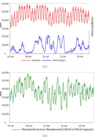
Fig. 2.3 presents a forecast of operating scenario of the GB network for year 2020 [57]. Fig. 2.3(a) shows the GB demand profile for January 2010, together with a scaled January 2010 wind generation. The blue line demonstrates the variability of the wind generation, with load factors ranging from 5% to 80%. The demand

(37)

profile is more consistent in respect of diurnal shape, but with lower levels across weekend and holiday periods. Assuming the same wind profile for January 2021 and an installed wind generation capacity of 26.7GW, Fig. 2.3(b) shows the expected variation in thermal generation output. Approximately 30GW change in thermal generation is expected within two days time frame. Additional thermal generation capacity must be allotted as reserve to cater for the variability in wind output. Fig. 2.4 shows the break up reserve requirement for secure operation of the system with the expected wind variability. Basic reserve, the reserve for forecast error and conventional generation capacity loss, and reserve for response, the reserve to support any in feed loss are common in power system operation. Variability in wind call for additional reserve capacity in conventional generating stations as indicated by blue shade. Higher reserve for response is also required to cater for sudden loss of large off-shore wind farms, towards the end of this decade.

Studies presented so far show that the flexibility required for generating stations is significantly higher compared to that of present day power system.

2.2.2

Changes in transmission system

A good transmission system is key to integration of renewable generation such as wind and solar. These resources are generally located in remote areas and weak transmission system can be a barrier to higher utilization of these resources [59, 60, 61]. Transmission system of various countries are transforming with installation of new HVDC lines and FACTS devices, and capacity improvement of existing lines to support power flow with increase in generation [62]. In UK, the majority of wind resource are located in Scotland whereas main load centers are located in England. Two HVDC lines are proposed along the Scotland-England transmission corridor to improve transfer capacity of the system [63]. Transmission lines connecting different energy resources can improve utilization of multiple energy resources depending on their output schedule. A meshed DC grid in the North Sea is found to result in increased utilization of wind and hydro capacity in the Norway and wind in the North Sea [5]. Also an ambitious plan to build a European supergrid is also under consideration [6] which will interconnect renewable resources in many countries with major load centers, enabling secure spread of electricity between the countries. An interconnection between different grids will reduce overall conventional reserve requirement in the system.

Another important development in recent years is the introduction of WAMS. Us-ing signals sent by the Global PositionUs-ing System satellites and Phasor measurement

(38)

(a)

(b)

Figure 2.3: Effect of wind penetration on thermal generation scheduling in GB network (a)GB demand and wind generation profile of January 2010 and (b) Thermal generation requirement for 2020. Source: [57]

units (PMU), WAMS can collect synchronized measurements from different parts of transmission network [64]. At present these measurements are use for post event analysis. However researchers are working towards using these measurements for real time monitoring and control of power system [65, 66]. WAMS will give a boost to development of more flexible transmission line operation.

2.2.3

Changes in distribution system

Distribution system is expecting a radical change in coming years with a shift from its passive nature of operation [67]. Using small scale wind turbines and solar panels at roof top, more customers will be producing part of their electricity by their own [68, 69]. Plug in electric vehicles and advanced home automation devices will further change the characteristics of distribution system. Future home will be more energy

(39)

Figure 2.4: Effect of wind penetration on operating Reserve Requirement in GB network for January 2020. Source: [57]

efficient. Moreover smart metering, and communication and computing capacity will be available to actively interfere in the system operation [70]. Using demand side management system the utilities can actively control system load [71]. The result will be a more stochastic nature in distribution system operation.

2.3

Chapter summary

The inter-area oscillations in power system depends on the operating condition of the system. Power system operation typically ensures that generator and transmission lines are loaded well below stability limit. However, for future power systems governed by market forces, power flow pattern will be decided by the price signals and weather conditions rather than technical boundaries. Integration of renewable generation will add additional stress into the system due to increased variability in operating conditions. Weather dependent nature of wind generation will increase operating reserve requirement and increase variability in conventional generation output. Since wind at different sites are less correlated as distance between sites increases, diversification of wind resources will reduce variability in total wind generation and as a result reduce variability in conventional generation. But it will increase the variation in power flow pattern in the system. The network must be flexible enough to face these scenarios. Transmission capacity enhancement is essential to provide the operating flexibility. Power systems around the world are installing many HVDC and FACTS devices to cope up with the changing operating conditions, which will increase the complexity of the network. The interaction of these devices when placed at close proximity, needs in depth study. The changes in

(40)

distribution system operation from its passive to active nature will add additional randomness in the system. The characteristics of evolving distribution system load and its effect on stability is not well understood. The increased complexity in network and variability in operating conditions will increase challenges for ensuring stability of the system for all operating conditions.

(41)

Chapter 3

Modeling and analysis of

multimachine power system

Modeling plays an important role in power system stability studies. Various components of the system should be modeled with sufficient accuracy to simulate the underlying physical phenomenon. This chapter details the modeling of power system from the perspective of small signal stability studies. Models of various power system components are adopted from [10, 72, 73]. The modeling details are limited to the context of this research work. The programming is carried out using MATLAB and Simulink software. The chapter also explains modal analysis and various control system tools used in stability analysis. A two-area test system is used to relate various terms used in the context of small signal stability.

3.1

Dynamic modeling of power system

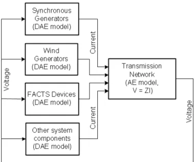
A model of power system is an integration of several dynamic models such as synchronous generators, asynchronous generators, load, FACTS devices, etc. Fig. 3.1 shows a top level view of the model, where various dynamic models are connected to a network model. The output of the network model is fed back to dynamic models making it a closed loop system. The network model consists of all transmission network components except the components modeled separately. It is represented using an algebraic equation V=ZI, where V is a vector of bus voltage, I is a vector of injected current at each bus and Z is a matrix representing the impedance of transmission line and other components not modeled separately. The output of the network block, bus voltage, is fed to dynamic models. The dynamic models consists of differential and algebraic equations (DAE), and the outputs are injected current

(42)

Figure 3.1: Overview of power system simulation program

at corresponding buses.

The power system networks used in this work contain dynamic models such as wind farms, synchronous generators, TCSC and SVC. The DAE equations for later three are listed in this chapter. Wind farm modeling is discussed in Chapter 4. Static load is assumed for all test systems as the objective of the work is to analyze impact of variable operating conditions resulting from large wind penetration on system stability. It is thought that this assumption will not cause significant error in the results and reduce complexity of the model. However, it is worth noting that the type and location of load will influence stability of power system and it is important to model dynamic load for accurate assessment of power system stability [10].

3.1.1

Synchronous machines

The modeling of synchronous generator is a subject matter of many text books and literatures [72, 73, 74]. The models of varying degree of complexity are reported. The modeling complexity required depends on the type of phenomena being studied and the available computational resource. This work uses transient model which is explained in this chapter. The model is sufficient for large system small signal stability studies if the model data is correctly determined [73]. However, subtransient model is required to analyze the behavior during subtransient period, and sub-subtransient model is important to analyze the effect of eddy current and asynchronous torque[75]. However for inter-area mode damping studies the use of these two models do not offer

(43)

significant improvement in accuracy compared to transient model [10]. Since the work is related to small signal stability studies in transient time period, the transient model having a field coil on d-axis and damper coil on q-axis is used. The governor is modeled using a reheat type turbine governor system and excitation system is represented using either a IEEE-DC1A or a IEEE-ST1A models.

Figure 3.2: Block diagram representation of synchronous machine model

Fig. 3.2 shows internal block representation of a synchronous machine model. The DAE equations corresponding to individual blocks are listed below. The input to synchronous machine model is bus voltage vDQ in (3.3) obtained from network block. The output of the model is current iDQ in (3.9) which is fed to the network block. A brief note on translating the differential equations or transfer functions to Simulink blocks is given in Appendix A. The various blocks are assembled to form synchronous machine model and later complete power system simulation program.

Equations for torque-angle loop block

dδi dt = ωi−ωs (3.1) dωi dt = ωs 2Hi [₋Di(ωi−ωs) +Tmi−Tei] (3.2) for i= 1,2,3...m, where,

m: total number of generators,

(44)

ωi: Speed of ith _generator

ωs: Synchronous speed of generator

Hi: Inertia of ith generator

Di: Damping coefficient of ith _generator Tmi: mechanical input torque of ith generator

Tei: electrical output torque of ith _generator

Equations for rotor electrical block

(vqi +jvdi) = vDQie−jδi = (vQi+jvDi)e−jδi (3.3)

dE′ qi dt = 1 T′ di0 [₋E_qi′ + (xdi−x ′ di)id+Ef di] (3.4) dE′ di dt = 1 T′ qi0 [−Edi′ −(xqi −x ′ qi)iqi] (3.5) dE_dci′ dt = 1 Tci [−E_dci′ −(x_qi′ −x′_di)iqi] (3.6) Equation (3.6) represents a dummy rotor coil used to handle transient saliency. A detailed discussion on treating saliency is available in [73].

(iqi+jidi) = 1 (Rai+jx ′ di) [E_qi′ +j(E_di′ +E_dci′ )₋(vqi+jvdi)] (3.7) Tei = E ′ diidi+E ′ qiiqi + (x ′ di−x ′ qi)idiiqi (3.8) iDQi = (iQi+jiDi) = (iqi+jidi)ejδi (3.9)

vqdi =vqi+jvdi: voltage in Park’s reference frame

vQDi =vQi+jvDi: voltage in Kron’s reference frame

iQDi =iQi+jiDi: current in Kron’s reference frame

E′

qi: transient emf due to field flux linkage

E′

di: transient emf due to flux linkage in q-axis damper coil

E′

dci: transient emf due to flux linkage in dummy rotor coil

idi: d-axis component of stator current

(45)

xdi, x

′

di: synchronous and transient reactance along d-axis, respectively

xqi, x

′

qi: synchronous and transient reactance along q-axis, respectively

T′

qi, T

′

di, T

′

ci: open circuit transient time constant along q-axis, d-axis and dummy coil, respectively

Excitation system block

Figure 3.3: Block diagram representation of excitation system model

The block diagram representation of DC type-1 excitation system is shown in Fig. 3.3 [72, 73]. VI and EF D are input, the measured voltage and output, the field voltage respectively. The constants KE and TE relate to exciter gain and time constant, respectively. The regulator transfer function has single time constant TA and positive gain KA. The feedback transfer function with constants KF and TF represent excitation system stabilizer, and the lead/lag block represent transient gain reduction. The figure can represent the static excitation system by setting the parameters, SE, KE, KF, and TF to zero.

Turbine governor block

Figure 3.4: Block diagram representation of turbine governor system model

Block diagram representation of governor with reheat steam turbine is shown in Fig. 3.4 [72]. The gain 1

R and the first order transfer function represent governor model and the other block represents reheat stream turbine model. The value of R

(46)

3.1.2

Thyristor controller series compensator (TCSC)

(a) (b)

(c) (d)

Figure 3.5: Various schematic representations of TCSC

A TCSC is formed of a Thyristor controlled reactor (TCR) connected in parallel with a fixed capacitor to provide rapid and continuous variation of transmission line series reactance. Fig. 3.5(a) shows a schematic representation of a transmission line with a TCSC, in which variable capacitor represents the TCSC. The compensated impedance of the transmission line is given by, Zth = R+jXL(1−kc/100), where

kc = XC_XL100 represents percentage compensation.

In dynamic modeling of the system, a TCSC can be represented using current injection model. The transformation of TCSC model from a variable series capacitor to injected current at terminal buses is depicted in Fig. 3.5(a) through Fig. 3.5(d) [12].

Let I be the current flowing from bus m to bus k. The TCSC having capacitive reactance XC can be represented by a voltage source VS = −jXCI as shown Fig. 3.5(b). The voltage source VS in Fig. 3.5(b) is replaced with a current source IS =

VS/(R+jXL) in Fig. 3.5(c). Further the current source IS is split into two current injections at terminal buses k and m as shown in Fig. 3.5(d).

Figure 3.6: Small signal dynamic model of TCSC

For small signal stability studies, the dynamic characteristics of TCSC can be modeled using a single time constant Ttcsc as shown in Fig. 3.6 [12]. Where, Ttcsc is

(47)

response time of TCSC,kc−ref is reference setting of TCSC andkc−ssis supplementary signal for damping control.

3.1.3

Static Var compensator (SVC)

Static var compensator is a shunt connected device which provides reactive power support to control dynamic voltage variations in the network. It consists of parallel combination of thyristor controlled reactor and fixed capacitors. The reactive power injection of a SVC at a bus k is given as,

Qk=Vk2Bsvc (3.10)

where Bsvc = BC −BL, and BC and BL are the susceptance of the fixed capacitor and thyristor controlled reactor, respectively. The corresponding current injection at bus k is,

Ik =jVkBsvc (3.11)

The small signal dynamic model of SVC is given in Fig. 3.7 [72]. Where,TSV C is the response time of the switching circuitry, TM is the time constant representing delay in measurement and Tv1 and Tv2 are the time constants of the voltage regulator block.

Figure 3.7: Small signal dynamic model of SVC

3.1.4

Initialization

The power system model presented above consists of non-linear equations which calls for a numerical solution. It is assumed that, the system is under stable equilibrium point (SEP) at timet= 0 and disturbance happens at t≥0. To start the simulation, it is necessary to calculate the initial value of states, x0 at timet= 0.

The primary step in initializing the model is to obtain a power flow solution of the network. The power flow solution gives real and reactive power output of generators

(48)