Remote sensing, numerical modelling and ground truthing for analysis of lake water quality and temperature

(1)

http://researchcommons.waikato.ac.nz/

Research Commons at the University of Waikato

Copyright Statement:

The digital copy of this thesis is protected by the Copyright Act 1994 (New Zealand).

The thesis may be consulted by you, provided you comply with the provisions of the Act and the following conditions of use:

 Any use you make of these documents or images must be for research or private study purposes only, and you may not make them available to any other person.

 Authors control the copyright of their thesis. You will recognise the author’s right to be identified as the author of the thesis, and due acknowledgement will be made to the author where appropriate.

 You will obtain the author’s permission before publishing any material from the thesis.

(2)

Remote sensing, numerical modelling and ground truthing for

analysis of lake water quality and temperature

A thesis

submitted in fulfilment

of the requirements for the degree of

Doctor of Philosophy in Biological Sciences at

The University of Waikato by

MATHEW GRANT ALLAN

(3)

(4)

iii Freshwater accounts for just 2.5% of the earth’s water resources, and its quality and availability are becoming an issue of global concern in the 21st century. Growing human population, over-exploitation of water sources and pressures of global warming mean that both water quantity and quality are affected. In order to effectively manage water quality there is a need for increased monitoring and predictive modelling of freshwater resources. To address these concerns in New Zealand inland waters, an approach which integrates biological and physical sciences is needed. Remote sensing has the potential to allow this integration and vastly increase the temporal and spatial resolution of current monitoring

techniques, which typically involve collecting grab-samples. In a complementary way, lake modelling has the potential to enable more effective management of water resources by testing the effectiveness of a range of possible management scenarios prior to implementation. Together, the combination of remote sensing and modelling data allows for improved model initialisation, calibration and validation, which ultimately aid in understanding of complex lake ecosystem processes.

This study investigated the use of remote sensing using empirical and semi-analytical algorithms for the retrieval of chlorophyll a (chl a), tripton, suspended minerals (SM), total suspended sediment (SS) and water surface temperature. It demonstrated the use of spatially resolved statistical techniques for comparing satellite estimated and 3-D simulated water quality and temperature.

An automated procedure was developed for retrieval of chl a from Landsat

Enhanced Thematic Mapper (ETM+) imagery, using 106 satellite images captured from 1999 to 2011. Radiative transfer-based atmospheric correction was applied to images using the Second Simulation of the Satellite in the Solar Spectrum model (6sv). For the estimation of chl a over a time series of images, the use of symbolic regression resulted in a significant improvement in the precision of chl a

(5)

iv hindcasts compared with traditional regression equations. Results from this

investigation suggest that remote sensing provides a valuable tool to assess temporal and spatial distributions of chl a. Bio-optical models were applied to quantify the physical processes responsible for the relationship between chl a concentrations and subsurface irradiance reflectance used in regression algorithms, allowing the identification of possible sources of error in chl a estimation. While the symbolic regression model was more accurate than

traditional empirical models, it was still susceptible to errors in optically complex waters such as Lake Rotorua, due to the effect of variations of SS and CDOM on reflectance.

Atmospheric correction of Landsat 7 ETM+ thermal data was carried out for the purpose of retrieval of lake water surface temperature in Rotorua lakes, and Lake Taupo, North Island, New Zealand. Atmospheric correction was repeated using four sources of atmospheric profile data as input to a radiative transfer model, MODerate resolution atmospheric TRANsmission (MODTRAN) v.3.7. The retrieved water temperatures from 14 images between 2007 and 2009 were validated using a high-frequency temperature sensor deployed from a mid-lake monitoring buoy at the water surface of Lake Rotorua. The most accurate temperature estimation for Lake Rotorua was with radiosonde data as an input into MODTRAN, followed by Moderate Resolution Imaging Spectroradiometer (MODIS) Level 2, Atmospheric Infrared Sounder (AIRS) Level 3, and NASA data. Retrieved surface water temperature was used for assessing spatial

heterogeneity of surface water temperature simulated with a three-dimensional (3-D) hydrodynamic model (ELCOM) of Lake Rotoehu, located approximately 20 km east of Lake Rotorua. This comparison demonstrated that simulations

reproduced the dominant horizontal variations in surface water temperature in the lake. The transport and mixing of a geothermal inflow and basin-scale circulation patterns were inferred from thermal distributions from satellite and model

estimations of surface water temperature and a spatially resolved statistical evaluation was used to validate simulations. This study has demonstrated the potential of accurate satellite-based thermal monitoring to validate water surface temperature simulated by 3-D hydrodynamic models.

(6)

v Semi-analytical and empirical algorithms were derived to determine spatial and temporal variations in SS in Lake Ellesmere, South Island, New Zealand, using MODIS band 1. The semi-analytical model and empirical model had a similar level of precision in SS estimation, however, the semi-analytical model has the advantage of being applicable to different satellite sensors, spatial locations, and SS concentration ranges. The estimations of SS concentration (and estimated SM concentration) from the semi-analytical model were used for a spatially resolved validation of simulations of SM derived from ELCOM-CAEDYM. Visual comparisons were compared with spatially-resolved statistical techniques. The spatial statistics derived from the Map Comparison Kit allowed a non-subjective and quantitative method to rank simulation performance on different dates. The visual and statistical comparison between satellite estimated and model simulated SM showed that the model did not perform well in reproducing both basin-scale and fine-scale spatial variation in SM derived from MODIS satellite imagery. Application of the semi-analytical model to estimate SS over the lifetime of the MODIS sensor will greatly extend its spatial and temporal coverage for historical monitoring purposes, and provide a tool to validate SM simulated by 1-D and 3-D models on a daily basis.

A bio-optical model was developed to derive chl a, SS concentrations, and coloured dissolved organic matter /detritus absorption at 443 nm, from MODIS Aqua subsurface remote sensing reflectance of Lake Taupo, a large, deep, oligotrophic lake in North Island, New Zealand. The model was optimised using in situ inherent optical properties (IOPs) from the literature. Images were

atmospherically corrected using the radiative transfer model 6sv. Application of the bio-optical model using a single chl a-specific absorption spectrum (a*ϕ(λ)) resulted in low correlation between estimated and observed values. Therefore, two different absorption curves were used, based on the seasonal dominance of

phytoplankton phyla with differing absorption properties. The application of this model resulted in reasonable agreement between modelled and in situ chl a concentrations. Highest concentrations were observed during winter when Bacillariophytes (diatoms) dominated the phytoplankton assemblage. On 4 and 5

(7)

vi March 2004 an unusually large turbidity current was observed originating from the Tongariro River inflow in the south-east of the lake. In order to resolve fine details of the plume, empirical relationships were developed between MODIS band 1 reflectance (250 m resolution) and SS estimated from MODIS bio-optical features (1 km resolution) were used estimate SS at 250 m resolution. Complex lake circulation patterns were observed including a large clockwise gyre. With the development of this bio-optical model MODIS can potentially be used to remotely sense water quality in near real time, and the relationship developed for B1 SS allows for resolution of fine-scale features such turbidity currents.

(8)

vii

List of Figures

Figure 1.1. Satellite and solar geometry. θ is azimuth angle, ᴕ is elevation angle and φ is zenith angle, which can be apply to either solar or sensor (view)

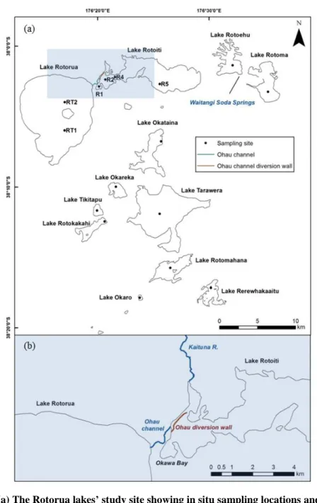
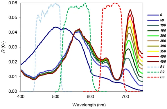
geometry. ... 4 Figure 2.1. (a) The Rotorua lakes’ study site showing in situ sampling locations and (b) the extent of expanded area represented with shading from (a), showing the location of the Ohau diversion wall, Lake Rotoiti. Each in situ sampling location corresponds to a 5 x 5 matrix (30-m pixels) average from Landsat ETM+ satellite images. ... 39 Figure 2.2. Modelled subsurface reflectance (R(0-)) for varying chlorophyll a concentrations ranging from 0 to 450 µg L-1_{with fixed CDOM absorption of 0.16}

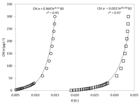
m-1 and tripton concentration of 0.5 mg L-1. The relative spectral response of Landsat bands B1, B2 and B3 is overlaid. ... 46 Figure 2.3. The semi-analytical relationship between chlorophyll (chl) a

concentrations and Landsat band-averaged subsurface irradiance reflectance R(0-) in B3 (open circles) and B2 (open squares) based on individual analytical

solutions. An exponential relationship (black line) is used to fit the analytical relationship with closeness of fit given by r2. This function was used to estimate chlorophyll a from R(0-). ... 47 Figure 2.4. Observed chlorophyll a (µg L-1_{) (y) versus estimated chlorophyll}_a_(x)

from the four different algorithms, plotted on a log-log scale. A 1:1 line (blue line), and r2 value are shown on each plot (n=87). (a) Symbolic regression algorithm equation: Chl a = (4618 B2 - 20)/((B1/B3)2) with r2=0.68 and RMSE=10.5 µg L-1. (b) Empirical algorithm equation: Chl a = exp(-2.12*(ln(B1/B3)) + 3.17) with r2=0.36 and RMSE=15.7 µg L-1. (c)

Semi-analytical model B2: Chl a = 0.0017e352.95 B2 with r2=0.58 and RMSE=13.8 µg L-1. (d) Semi-analytical model B3: Chl a = 0.36e447.13 B3 with r2=0.58 and RMSE=14.1 µg L-1. ... 49

(15)

xiv Figure 2.5. Modelled subsurface reflectance (R (0-)) for varying tripton

concentrations ranging from 0 to 9 mg L-1_{, with fixed CDOM absorption of}_0.16

m-1 and chl a concentration of 20 µg L-1_{. The relative spectral response of Landsat}

bands B1, B2 and B3 is overlaid. ... 50 Figure 2.6. Modelled subsurface reflectance (R(0-)) for varying CDOM

absorption ranging from 0 to 1.8 m-1_{, with fixed tripton concentrations of 0.5 mg}

L-1 and chl a of 20 µg L-1_{. The relative spectral response of Landsat bands B1, B2}

and B3 is overlaid... 50 Figure 2.7. Time series plots of estimated chlorophyll a (µg L-1_{) from the}

symbolic regression (closed circles) and from all in situ data (open circles) for Lake Rotoma (a), Lake Rotoehu (b), and Lake Rotorua (c). Note that in most cases dates of in situ and satellite sampling dates are not identical. ... 52 Figure 2.8. Chlorophyll a concentration (µg L-1_{) in Lake Rotoehu derived from}

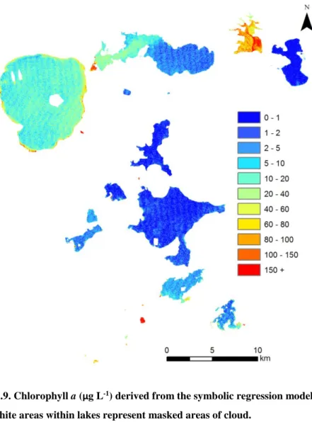
the symbolic regression model. ... 54 Figure 2.9. Chlorophyll a (µg L-1_{) derived from the symbolic regression model on}

24 January 2002. White areas within lakes represent masked areas of cloud... 55 Figure 2.10. Chlorophyll a (µg L-1_{) derived from the symbolic regression model}

in north-western Rotorua lakes on selected dates with high spatial variation. Note: some lakes were removed due to cloud cover. ... 56 Figure 3.1. Study site map including depth for (a) Rotorua lakes and (b) Lake Taupo... 75 Figure 3.2. Lake Rotoehu study site, showing the location of the water quality monitoring station, and the Waitangi Soda Springs inflow plume zone for

comparison of ELCOM and Landsat temperature data... 75 Figure 3.3. Comparison of relative humidity versus pressure profiles from four sources of atmospheric data used in MODTRAN on two different dates: (a) 27 January 2009 and (b) 8 September 2009. ... 83 Figure 3.4. Landsat-estimated temperature (ºC) on 20 June 2009 using radiosonde atmospheric data in (a) Rotorua lakes, and (b) Lake Taupo. The stripes of missing data caused by the failure of the scan line corrector have been filled using linear interpolation. ... 84 Figure 3.5. Landsat-estimated temperature (ºC) on 25 January 2008 using

(16)

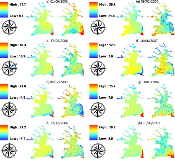
xv missing data caused by the failure of the scan line corrector have been filled using linear interpolation. ... 85 Figure 3.6. Surface water temperature simulations at the BOPRC monitoring site using Rotorua Airport meteorological temperature data (ELCOM), modified temperature data (using equation 3.5) (ELCOM modified met), in situ temperature and Landsat-derived temperature data (radiosonde). ... 87 Figure 3.7. Mean water surface temperature in the Waitangi Soda Springs

geothermal plume zone of Lake Rotoehu estimated by Landsat (black line)

compared that simulated (dashed line). ... 87 Figure 3.8. ELCOM surface water temperature simulation (column 1 and 3), Landsat-derived water surface temperature (columns 2 and 4) with standard deviation stretched colour ramp (ºC). Wind speed and direction are represented on the compass plot with compass radius representing a wind speed of 10 m s-1, compass north direction is zero degrees... 89 Figure 3.9. Landsat-estimated surface water temperature of Lake Rotoehu on (a) 1 September 2006 and (b) 17 September 2006 and visualization of ELCOM-simulated tracer on the corresponding dates of (c) 1 September 2006 with 25% and (d) 17 September 2006 (25%). The percent tracer concentration is relative to 100% tracer concentration in the inflow. ... 90 Figure 4.1. Study site Lake Ellesmere (overlaid on a Landsat 5 background captured 2 July 2005) showing inflows, outlet, mid-lake grab-sampling site, Kaituna Lagoon and Kaitorete Spit. ... 104 Figure 4.2. Relationship between non-algal volatile suspended sediment

(NAVSS) and tripton concentration (CTR) in Lake Ellesmere (r2=0.92, n=12) from 9 July 2008 to 1 September 2008. ... 115 Figure 4.3. Relationship between MODIS reflectance and tripton concentration (CTR) (mg L-1). The line shows the linear regression with r2=0.61 and p<0.0001. ... 115 Figure 4.4. (a) The analytical relationship between tripton concentrations as a function of MODIS subsurface remote sensing reflectance (rrs(B1)) represented by open grey circles. An exponential relationship is used to approximate the analytical relationship (black line). This function was used to estimate tripton

(17)

xvi concentration from MODIS rrs(B1). (b) Graph of the same relationship as (a) but extended over a larger range of tripton concentrations. ... 117 Figure 4.5. In situ concentration of tripton and estimates using (a) the semi-analytical model (RMSE=58.4 mg L-1) and (b) empirical model (RMSE=58.9 mg L-1). A 1:1 line (grey) and the observed vs. estimated regression equation and line (black) and associated r2 are shown on each plot (n=9). ... 117 Figure 4.6. Suspended mineral (SM) concentrations (mg L-1) simulated using the 1-D model (line), measured with situ grab-samples (closed circles) and estimated from remote sensing (open circles) for the period 1 March 2006 to 31 August 2007. ... 118 Figure 4.7. Simulated concentrations of suspended minerals (SM) (mg L-1) using the 3-D model (black line) and 1-D model (dashed line), in situ concentrations (closed circles for the period 1 December 2006 to 11 March 2007), and satellite-estimated concentrations (open circles). Average hourly wind speed (m s-1) is represented by the grey line. ... 119 Figure 4.8. Suspended mineral concentration (mg L-1) estimated from MODIS data (left) and from 3-D model simulations (right). Note colour scale differences in some instances. Hourly average wind speed and direction are plotted on the wind rose, with changes in colour representing wind speed. ... 124 Figure 5.1. Lake Taupo study site. (a) Sites A , B and C represent water quality monitoring stations used in this study and bathymetry contours (m) are shown as a colour gradient from blue (shallow) to red (deep). (b) Tongariro/Tokaanu inflows and locations of Turangi meteorological station and Tongariro flow gauge at Major Jones. ... 148 Figure 5.2. Chlorophyll absorption cross section with wavelength. Black line is the lowest absorption measured by Belzile (2004), and the dashed line is from the Bacillariophyte Chaetoceros protuberans (Sathyendranath et al. 1987). ... 155 Figure 5.3. Plots of field data used in this study from 1 February to 14 March 2004. (a) Hourly rainfall (mm) and Tongariro River flow from 27 February to 6 March 2004 (m3 s-1) measured at Turangi. (b) Hourly wind speed (m s-1) measured at Turangi. (c) Interpolated thermistor chain data (oC) from Site B in Lake Taupo. ... 157

(18)

xvii Figure 5.4. Secchi depth (m) from 19 November 2003 to 10 June 2004 from Site A (unshaded disk symbol) and Site B (shaded disk symbol). ... 158 Figure 5.5. In situ versus MODIS-estimated chlorophyll a. The line denotes the regression relationship (satellite-estimated chl a = 0.741 (In situ chl a) + 0.356) using a seasonally adjusted chlorophyll specific absorption coefficient (n = 23, r2 = 0.71, p<0.01, root mean squared error (RMSE) = 0.522 µg L-1). The estimations using the a*ϕ(λ) from Belzile (2004) are shown with a diamond, and using a*ϕ(λ) from the Bacillariophyte Chaetoceros protuberans (Sathyendranath et al. 1987) shown with a square. ... 159 Figure 5.6. MODIS-derived chl a (µg L-1), CDOMD absorption (abs) (m-1) at 443 nm and SS (mg L-1)on 3 August 2004. A grey-coloured buffer is used from the lake edge to 1500 m into the lake, to avoid possible areas of bottom reflectance and stray light from regions close to the shoreline. ... 160 Figure 5.7. MODIS-derived chl a (µg L-1), CDOMD absorption (abs) (m-1) at 443 nm and SS (mg L-1)on 4 March 2004. The white oval shape is used to mask a small area of cloud, and a grey-coloured buffer is used from the lake edge to 1500 m into the lake, to avoid possible areas of bottom reflectance and stray light from regions close to the shoreline. ... 161 Figure 5.8. MODIS-derived chl a (µg L-1_{), CDOMD absorption (abs) (m}-1_{) at 443}

nm and SS (mg L-1₎_{on 5 March 2004. A grey-coloured buffer is used from the}

lake edge to 1500 m into the lake, to avoid possible areas of bottom reflectance and stray light from regions close to the shoreline. ... 162 Figure 5.9. MODIS band 1 SS calculated from eq. 5.8 and 5.9, on 4 and 5 March 2004. The white oval shape shows areas where cloud has been masked. ... 163 Figure 5.10. Photograph of Lake Taupo taken from c. 3000 m above Taupo Airport on the north eastern shore looking towards the south-west shore (Photo by Jonathan King, 5 March 2004). ... 164

(19)

xviii

List of Tables

Table 2.1. Lake and catchment characteristics of the Rotorua lakes Source: (Scholes and Bloxham 2008; Scholes 2011). ... 40 Table 2.2. Coefficient of determination (r2) for regression relationships between in situ chlorophyll a and Landsat bands 1-4. * represents p>0.05 (n=87). ... 48 Table 3.1. Root-mean-square-error (RMSE) and mean difference between in situ measured water temperature (Lake Rotorua buoy) and Landsat-derived

temperature using different sources of atmospheric data over 14 separate dates (RASO - radiosonde, ML2 - MODIS Level 2, AL3 - Airs Level 3). ... 81 Table 3.2. Error in temperature estimation in Lake Rotorua (estimated –

measured, oC) for different AC methods (RASO - radiosonde, ML2 - MODIS Level 2, AL3 - Airs Level 3) and relative humidity (RH) measured at the Rotorua meteorological station. ... 82 Table 4.1. ELCOM-CAEDYM parameters related to suspended mineral (SM) resuspension and sedimentation. ... 114 Table 4.2. Statistical comparison of SM concentrations estimated from the semi-analytical algorithm and simulated from the 3-D model (n = 2414 for each instance). Statistical fit is represented using r2 values based on linear regression, Geographically Weighted Regression (GWR r2), Fuzzy Numerical Statistic (FNS), Wavelet Verification Algorithm (WVA r and WVA RSE), and Warping Defamation Penalty Statistic (WDPS). Relationships that were not significant (p > 0.05) were represented by *. ... 123

(20)

xix

List of acronyms

3-D Three-dimensional

6sv Second Simulation of a Satellite Signal in the Solar Spectrum

AC Atmospheric Correction

AIRS Atmospheric InfraRed Sounder

AOD Aerosol Optical Depth

AOPs Apparent Optical Properties

BIOPTI Bio-optical model for inland waters BOPRC Bay of Plenty Regional Council

BRDF Bi-directional Reflectance Distribution Function CAEDYM Computational Aquatic Ecosystem Dynamics Model CDOM Coloured Dissolved Organic Matter

CZCS Coastal Zone Colour Scanner

DN Digital Number

DYRESM DYnamic REservoir Simulation Model

ELCOM Estuary Lake and Coastal Ocean Model

ESA European Space Agency

ETM+ Enhanced Thematic Mapper Plus

GIS Geographic Information System

GloVis GloVis

GWR Geographically Weighted Regression

IDL Interactive Data Language

IOPs Inherent Optical Properties

IR Infrared

LDCM Landsat Data Continuity Mission

LMM Linear Mixture Modelling

LOWTRAN LOW Resolution TRANsmission model

MCK Map Comparison Kit

MERIS MEdium Resolution Imaging Spectrometer

MNF Minimum Noise Function

MODIS MODerate Resolution Imaging Spectroradiometer MODTRAN MODerate resolution atmospheric TRANsmission

NAP Non-Algal Particles

NASA National Aeronautics and Space Administration NAVSS Non-Algal Volatile Suspended Sediment

NIR Near Infrared

NIWA National Institute of Water and Atmospheric Research

(21)

xx

NZST New Zealand Standard Time

OACs Optically Active Constituents PAR Photosynthetically Active Radiation

RH Relative Humidity

RMSE Root Mean Squared Error

SM Suspended Minerals

SNR Signal-to-Noise Ratio

SPOT Système Probatoire d’Observation de la Terre SS Total Suspended Sediment or particles

TLTMP Taupo Long Term Monitoring Programme

TM Thematic Mapper

TOA Top Of Atmosphere

VSS Volatile Suspended Sediment

(22)

xxi

List of symbols

a(λ) Spectral absorption coefficient (m−1)

a*TR(λ) Specific absorption coefficient of tripton (m2 g −1) a*ϕ(λ) Chlorophyll-specific absorption coefficient (m2 mg −1) aCDOM(λ) CDOM absorption coefficient (m−1)

aCDOMD(λ) CDOM and detritus absorption coefficient (m−1) aw(λ) Pure water absorption coefficient (m−1)

b(λ) Spectral scattering coefficient (m−1)

b*SS(λ) Specific scattering coefficient of SS (m2 g −1) b*

TR(λ) Specific scattering coefficient of tripton (m2 g −1)

b*ϕ(λ) Specific scattering coefficient of phytoplankton (m2 mg −1)

bb(λ) Spectral backscattering coefficient (m−1) BbSS Backscattering ratio of suspended sediment BbTR Backscattering ratio of tripton

bbw(λ) Backscattering coefficient of pure water (m−1) Bbϕ Backscattering ratio of phytoplankton

Br Landsat bias (W m-2 sr-1 µm-1)

CSM Concentration of suspended minerals (mg L-1) CTR Concentration of tripton (mg L-1)

Cϕ Concentration of chl a (µg L-1)

E(λ) Irradiance (W m−2 nm−1)

Ed(λ) Downwelling irradiance (W m−2 nm−1) Eu(λ) Upwelling irradiance (W m−2 nm−1)

g0, g1, r1 Factors relating rrs(λ) and R(0-) to a and bb (sr−1) Gr Landsat rescaled gain (W m-2 sr-1 µm-1/DN) L(λ) Spectral radiance (W m−2 nm−1 sr−1)

La(λ) Atmospheric or upwelling radiance emitted/scattered by the atmosphere (W m-2_sr-1_µm-1₎

Lr(λ) Radiance due to multiple scattering by air molecules (Rayleigh) (W m−2 nm−1 sr−1)

Lt(λ) _{At-sensor radiance (W m}-2_sr-1_µm-1₎ Ls(λ) Surface leaving radiance (W m−2 nm−1 sr−1)

(23)

xxii Lsky

Downwelling or sky radiance reflected from the surface (W m-2 sr-1 µm-1)

Lu(λ,z), Lw(λ) Upwelling radiance (W m−2 nm−1 sr−1)

Lw(λ) Water leaving radiance (W m−2 nm−1 sr−1) n Scattering exponent of tripton or SS ᴕ Elevation angle (o)

ơL Fresnel reflectance (sr−1) ⱷ Azimuth angle (o)

R(0-)(λ) Subsurface irradiance reflectance

R(0+)(λ) Above water surface irradiance reflectance

Rrs(λ), rrs(λ) Above, below water surface remote sensing reflectance (sr−1) Rv gas constant for moist air = 461.5 J kg-1

S Spectral slope coefficient of CDOM (nm-1) τ(λ) _{Atmospheric transmittance}

z Depth (m)

β(θ) volume scattering function (m−1 sr-1₎

β(θ) Volume scattering function (m-1 sr-1), where θ is forward scattering angle

ε Emissivity of the water surface θ Zenith angle (o)

θ forward scattering angle (o)

λ, λ0 Wavelength, reference wavelength (nm)

Q The amount of energy held by a photon (J) h Plank’s constant (J s-1)

v Frequency (Hz)

(24)

xxiii

Acknowledgments

First and foremost I would like to thank my chief supervisor Professor David Hamilton for his constant enthusiasm and tireless effort in supervising this project. Thanks to my lovely partner Tineke Webley for your support and patience. I thank my co-supervisors Associate Professor Brendan Hicks and Dr Lars Brabyn. I also thank the following collaborators; Dr Dennis Trolle in chapters 3 and 4, Kohji Muraoka in Chapter 3, and Dr Max Gibbs in Chapter 5. Dr Deniz Özkundakci provided valuable technical advice on many aspects of this thesis. Jonathan Abell provided feedback on drafts and technical advice.

Funding was provided by the Bay of Plenty Regional Council (BOPRC) and the Ministry of Science and Innovation (contract UOWX0505). This work benefited from participation in the Global Lakes Ecological Observatory Network

(GLEON).

I thank BOPRC for providing the measured data for water quality variables, in particular Glenn Ellery, Paul Scholes, and Gareth Evans. Dr Salman Ashraf, Dr Kevin Collier (Environment Waikato) and Associate Professor Lex Chalmers (University of Waikato), who provided valuable advice on data analysis. Dr Matt Pinkerton (National Institute of Water and Atmospheric Research, New Zealand) provided technical guidance on satellite platforms and capability. Julia Barsi (NASA) provided the Interactive Data Language (IDL) code to apply spectral response functions to MODTRAN output and created the NASA atmospheric correction tool used in this study. Chris McBride (University of Waikato)

provided data from a monitoring buoy on Lake Rotorua. Dr Hirokazu Yamamoto (Advanced Industrial Science and Technology, Japan) gave valuable feedback on atmospheric correction calculations. Graeme Plank (University of Canterbury Physics Department) provided weather station data from Birdlings Flat under difficult circumstances soon after the Canterbury earthquake. Dr Stéphane Maritorena (University of California Santa Barbara) provided valuable advice in

(25)

xxiv adapting the bio-optical model for image applications and provided a MODIS Aqua version of the bio-optical model code. Jonathan King provided the aerial image of Lake Taupo. Associate Professor Hiroshi Yajima provided valuable technical assistance in 3-D modelling.

This thesis is dedicated to my late father James Grant Allan, who I know was proud at seeing this Ph.D. near its completion.

(26)

xxv

Preface

This thesis is comprised of six chapters which present the results relating to this study, relevant literature and discussion. Chapters 2-5 have been written for publication in peer-reviewed scientific journals. Except where referenced, I conceived the work presented in this thesis, including data analysis, interpretation and writing, undertaken while under the supervision of Professor David P.

Hamilton (University of Waikato).

Chapter 2 is in preparation for submission to a peer reviewed journal under the title ‘Remote sensing of chlorophyll a concentrations in Rotorua lakes of New Zealand’ by Mathew Allan, David P. Hamilton, Brendan Hicks and Lars Brabyn.

Chapter 3 has been submitted to Remote Sensing of Environment under the title ‘Atmospheric correction of Landsat thermal imagery for surface water

temperature retrieval and three-dimensional hydrodynamic model validation of spatial heterogeneity in geothermally-influenced lakes’ by Mathew Allan, David P. Hamilton, Dennis Trolle, Kohji Muraoaka and Chris McBride. David Hamilton assisted with planning and editing, Dennis Trolle assisted with model creation, Kohji Muraoaka created the 3-D visualisation, and Chris McBride manufactured the buoy.

Chapter 4 is in preparation for submission to a peer reviewed journal under the title ‘MODIS-based estimates of suspended minerals to evaluate performance of a three-dimensional hydrodynamic-ecological model application to a large, shallow coastal lagoon’ by Mathew Allan, David P. Hamilton and Dennis Trolle. David Hamilton assisted with planning and editing, Dennis Trolle provided the original 1-D model which was modified, and with my help, set up the 3-D model, which was then modified.

(27)

xxvi Chapter 5 is in preparation for submission to a peer reviewed journal under the title ‘Optimization of a semi-analytical model for remote sensing of Chlorophyll a in a large oligotrophic lake using MODIS’ by Mathew Allan, David P. Hamilton and Max M. Gibbs. Daivd Hamilton assisted with planning/editing, and Max Gibbs provided in situ data and assisted with editing.

(28)

1

1 General introduction

1.1 Motivation

Eutrophication

Eutrophication is generally defined as an increase in nutrients such as phosphorus and nitrogen which enhance algal growth (Wetzel 2001), leading to a decrease in water quality. It is a natural process whereby with age lakes gradually infill with sediment, nutrients, and organic matter. Human induced changes within catchments can speed up this natural process, which is then termed cultural eutrophication. Cultural eutrophication can result in decreased water clarity, harmful algal blooms, increased suspended sediment, hypoxia and anoxia, losses or increased growth of submerged macrophytes and lake biota, and, ultimately, risks to human health (Williamson et al. 2008). Lakes can be thought of as integrators of environmental change which has occurred within their catchments (Williamson et al. 2008).

Remote sensing and modelling solutions

Methods to assess water quality may be categorised into three main types; in situ sampling, numerical modelling and remote sensing (Dekker et al. 1996). In situ methods using grab-samples are generally suited to monitoring at low temporal resolution. By contrast autonomous water quality sensors allow for monitoring at high frequency and potentially in real time. However, neither of these methods is well suited to effectively capturing horizontal heterogeneity of water quality and temperature.

Remote sensing can provide synoptic monitoring of optically active water constituents (e.g., Kloiber et al. 2002) and may therefore allow monitoring of

(29)

2 temperature and optically active water quality variables at high spatial resolution (e.g., Dekker et al. 2002; Binding et al. 2007). Furthermore it can be accomplished at near real time in cases where satellite overpasses occur daily.

Three-dimensional (3-D) and one-dimensional (1-D) hydrodynamic and thermodynamic modelling of lake water temperature offers an opportunity to

interpolate temporal gaps in data derived from satellite and traditional monitoring of water quality and temperature, and to extend the analysis to the vertical domain (Hedger et al. 2002). When coupled to ecological models, this modelling may also provide insights into the spatial variability of biogeochemical processes (Jorgensen 2008).

The synthesis of data derived from remote sensing, modelling and in situ sampling provides an unparalleled opportunity for understanding ecosystem structure and function. Horizontal validation of 3-D models with traditional point-based monitoring is often limited by the synoptic coverage and quantity of field data. Remote sensing therefore has the potential to provide a cost effective method for synoptic validation. Modelling provides an opportunity for interpretation of remotely sensed imagery through the quantification of the physical and biological fluxes that redistribute variables and lead to the spatial distributions observed through remote sensing.

However, there are some inherent limitations of remote sensing. Use of visible and infrared (IR) radiation of from lakes is not possible during periods of cloud cover, which is a frequent occurrence in New Zealand. Remote sensing is unable to derive estimates of non-optically active water constituents, such as nutrient concentrations. Measurements of total radiance from satellites may comprise up to 90% atmospheric path radiance, making it difficult to quantify radiance from optically active

constituents (OACs) of water (Vidot and Santer 2005), therefore atmospheric correction is essential for the standardisation of a time series of images. In optically complex Case 2 waters found in lakes, at least three optically active constituents influence reflectance, and these constituents can vary independently from each other (Bukata et al. 1995). The retrieval of water constituent concentrations from Case 2

(30)

3 waters is therefore more demanding in terms of algorithm complexity and the

required level of satellite sensor spectral resolution (Matthews 2011).

Water quality monitoring in New Zealand

Of the 3820 lakes larger than one hectare in New Zealand, only 3% (117) are monitored as part of a long-term programme. Forty-four percent of the monitored lakes were recently found to be eutrophic and 33% oligotrophic (Verburg et al. 2010). In past and present monitoring programmes, lake trophic state is reported for 134 lakes (Hamill 2006). Water quality monitoring in New Zealand currently uses traditional monitoring techniques involving collection of a water grab-sample from one site in a lake or occasionally from multiple sites in larger lakes, and subsequent laboratory analysis. Other measurements may be made in situ, such as Secchi depth and profiles of temperature, turbidity, light or dissolved oxygen. Laboratory

sampling methods are time-consuming and expensive, with results often not available for considerable time periods after the sample is taken. The small percentage of lakes monitored in New Zealand is indicative of the high cost associated with traditional point sample collection and subsequent analysis.

Remote sensing theory

Remote sensing is the science of obtaining information about an object using a device that is not in contact with that object (Bukata et al. 1995). According to this definition, remote sensing was practiced by the pioneers of astronomy such as Galileo and Copernicus. Modern environmental remote sensing has its roots in the military reconnaissance of World War I (Bukata et al. 1995). Remote sensing has subsequently benefited from technological advances emerging from space

exploration programs (Bukata et al. 1995).

Passive remote sensing involves sensors that record electromagnetic (EM) energy reflected or emitted by the earth. The energy can be modelled either as a wave or as a particle which travels at the speed of light. The most important characteristic of EM for the purpose of remote sensing is the wavelength (λ). Longer wavelengths are

(31)

4 associated with lower frequency and energy according to Equation 1.1 which defines Q, the amount of energy held by a photon (measured in joules), as:

𝑄 = ℎ 𝑣 = ℎ 𝑐_λ (1.1)

where h is Planck’s constant, v is frequency, and c = 2.998 × 108 m s-1.

Remote sensors record EM in the form of radiance, L(θ, φ, λ), which is defined as the radiant flux per unit solid angle per unit area at right angles to the direction of EM propagation (W m-2 sr-1), with a specified azimuth (θ) and zenith (φ) angle. Radiance is a subset of irradiance E(λ), which is defined as the total radiative flux incident upon a point on a surface from all directions above the surface. The geometry associated with a remote sensing instrument is shown in Figure 1.2.

Figure 1.1. Satellite and solar geometry. θ is azimuth angle, ᴕ is elevation angle and φ is zenith angle, which can be apply to either solar or sensor (view) geometry.

(32)

5 The simplified radiance recorded by a remote sensor can be expressed as (assuming no adjacency effects or bottom reflection):

Lt(θv, φv, θs, λ) = Lr(θv, φv, θs, λ) + La(θv, φv, θs, λ) + Tatm(θv, θs, λ)Ls(θv, φv, θs, λ) (1.2)

where:

Lr(λ) = radiance due to multiple scattering by air molecules (Rayleigh scattering) La(λ) = radiance from multiple scattering of aerosols

Tatm(λ) = atmospheric transmittance from water to sensor Ls(λ) = surface leaving radiance

λ = wavelength

θv = view or observation zenith angle φv = view azimuth angle

θs = solar zenith angle

Adjacency effects are caused by reflection from a non-target area (e.g. land) being scattered into the field of view by the atmosphere. If the non-target area is brighter than the target, there will be an increase in the apparent brightness of the target area, and a reduction of image contrast (Santer and Schmechtig 2000).

Surface-leaving radiance, Ls(θv, φv, θs, λ), is estimated through applying an

atmospheric correction, described below. Water-leaving radiance is estimated from (Kallio 2012):

Lw(θv, φv, θs, λ) = Ls(θv, φv, θs, λ) - ơLLsky(θv, φv, θs, λ) (1.3)

where:

Lsky(θv, φv, θs, λ) = sky specular reflectance at sensor ơL = Fresnel reflectance

(33)

6 ) ( ) , , , ( ) , , , (          d s v v w s v v rs E L R  (1.4)

where Edis downwelling irradiance immediately above the water surface. Subsurface remotely sensed reflectance rrs(λ) can be estimated from Rrs(λ) by correcting for air-water interface effects, assuming a nadir viewing sensor and optically deep waters (Lee et al. 2002):

) ( 7 . 1 52 . 0 ) ( ) (    rs rs rs R + R r  (1.5)

The general term reflectance used in this thesis refers to rrs(λ). Subsurface irradiance reflectance R(0-)(λ) is given as (depth=0, spectrally dependant):

 

u d E E = R 0 (1.6)

where Eu is upwelling radiance.

Atmospheric correction of remote sensing data

Atmospheric correction is a crucial step in any time series analysis of satellite imagery as a satellite only captures a fraction of radiation coming from a target. Radiance recorded by remote sensing can be comprised of greater than 90% path radiance, which originates from scattering of solar radiation by air molecules and aerosols (suspended liquid and particles such as salt, dust, ash, pollen and sulphuric acid) (Vidot and Santer 2005). These molecules and particles can also attenuate radiation through absorption. Scattering can occur multiple times and there is variability of aerosol particulate distributions (Bukata et al. 1995), resulting in complex photon paths.

There are various methods of atmospheric correction, including radiative transfer modelling correction, image based correction and vicarious calibration correction.

(34)

7 Vicarious calibration involves measuring solar irradiance and reflectance

concurrently with satellite overpass. The most common image-based atmospheric correction to estimate Ls involves dark object subtraction (DOS), in which the darkest pixel in each band is used as an estimate of path radiance, and is subtracted from radiance at the top of the atmosphere (Chavez 1996).

The application of radiative transfer models offers the flexibility to address the complexities of atmospheric correction over inland waters (e.g., Campbell et al. 2011). Such complexities include variations in elevation, which affect molecular calculations due to changes in air pressure, and adjacency effects. In addition, heterogeneous concentrations of aerosols and aerosol content at coastal and inland locations needs to be considered, although it is often assumed that aerosol optical depth (AOD) is homogenous at spatial scales of 50 to 100 km (Vidot and Santer 2005). There is also interaction of absorption and scattering, and the radiative transfer model must provide a complete description to provide accurate simulation. Gaseous absorption is therefore calculated for each scattering path whilst absorption is computed as a simple multiplicative factor. The principal absorbing gases are oxygen, ozone, water vapour, carbon dioxide, methane, and nitrous oxide, of which ozone and water vapour are assumed to vary most in time and space (Kotchenova et al. 2008). The calculation of scattering is much more complex, and includes

contributions from Rayleigh and aerosols. Second Simulation of a Satellite Signal in the Solar Spectrum (6sv) (Kotchenova et al. 2008) is a radiative transfer atmospheric correction code accounting for radiation polarization, which enables accurate

simulations of satellite and airborne observations, accounting for a molecular and aerosol mixed atmosphere.

An alternative approach to atmospheric correction of ocean colour data is the use of the SeaDAS range of atmospheric correction procedures (Ruddick et al. 2000; Wang et al. 2009; Bailey et al. 2010), which preserve the near infra-red (NIR) reflectance peak (Odermatt et al. 2012a). However, this procedure can return negative

reflectance at blue wavelengths over turbid or inland waters (Goyens et al. 2013). A promising alternative, which obviates negative reflectance, is a neural network (NN) based inversion approach (Schroeder et al. 2007), which has been shown to

(35)

8 outperform SeaDAS atmospheric correction algorithms over turbid waters (Goyens et al. 2013).

Water colour theory

The colour and clarity of water depend on its optical character, and relate to the bulk optical processes of absorption and scattering (Davies-Colley et al. 1993).

Absorption and scattering characteristics of water are determined by inherent optical properties (IOPs). Absorption refers to the transfer of light energy into another form of energy (e.g., heat) and is quantified by the spectral absorption coefficient, a(λ) (m -1_{), which is the fraction of incident light absorbed divided by the thickness of the}

layer. Scattering is defined as deflection of light photons from their original path (Davies-Colley et al. 1993), and can be quantified by the spectral scattering coefficient, b(λ) (m-1), which is the fraction of the incident light which is scattered divided by the thickness of the layer (Kirk 2010). Light scattering is also quantified by the volume scattering function (β(θ)), where θ is the forward scattering angle (Mobley 1994). The integral of β(θ) for angles from 0 to π yields b:

     d b 2 ( )sin( ) 0



 (1.7)

The backscattering coefficient is a subset of the angle used to define b:

       d b_b 2 ( )sin( ) 2 /



 (1.8)

The backscattering ratio Bb is defined as bb (λ)/b(λ).

Apparent optical properties (AOPs) are determined by the combined effects of the geometric structure of the light field and water constituents (Kirk 2010). They are therefore partly determined by the solar zenith angle and local atmospheric conditions (Bukata et al. 1995). The underwater vertical attenuation coefficient, Secchi depth and irradiance reflectance are considered to be AOPs (Preisendorfer

(36)

9 1976; Mobley 1994). In contrast IOPs are affected only be the medium, and radiative transfer theory describes the connection of IOPs and AOPs (Mobley 1994). The IOPs of a water body are completely quantified by the β(θ) and a(λ) (Mobley 1994). Clear water in natural ecosystems contains low concentrations of optically active constituents. Consequently the spectral reflectance is low and the spectral shape is similar to that for pure water molecules. It shows an exponential increase in absorption towards longer wavelengths and an increase in scattering at shorter wavelengths of the visible range of the electromagnetic spectrum (Rudorff et al. 2006).

Algae-laden water exhibits a reflectance peak in the green region, which represents an aggregate chl absorption minimum, and another reflectance peak at 700 nm. Absorption troughs occur in the blue and red/ IR wavelength range (Han 1997), with the exact location and width of these troughs dependent on phytoplankton species’ assemblages and their physiological state (Kirk 2010). Fluorescence is an optical process which involves the absorption of part of the energy of a photon and re-radiation of a lower energy photon in an arbitrary direction, which can sometimes influence the colour of natural waters (Davies-Colley et al. 1993). Phytoplankton displays a fluorescence peak centred at 685 nm, meaning concentrations can be measured using fluorometers when photoreaction centres are not saturated (Yentsch and Yentsch 1979).

Tripton includes sand, silt, clay and other inorganic material such as atmospheric dust (Koponen 2006), as well as non-living organic matter. The optical properties of tripton are affected by the shape and size distribution of particles, which have a major effect on their absorption and scattering properties (Bukata et al. 1995). In clear water, increasing concentrations of tripton result in a linear increase in reflectance in the IR, with a coefficient of variation near to one. In this area of the electromagnetic spectrum the effect of chlorophyll (chl) a is negligible (Han 1997). In algae-laden water, additive effects of tripton on reflectance occur at all

(37)

10 The absorption spectrum of coloured dissolved organic matter (CDOM) increases exponentially at shorter wavelengths of the visible spectrum and there is little absorption above 700 nm (Bricaud et al. 2009). The effect of CDOM on light scattering is minimal and can be ignored (Koponen 2006).

Methods of remote sensing of water quality

In Case 1 waters where variation in rrs(λ) is primarily due to phytoplankton, simple empirical band ratio models can be used to determine chl a (Gordon and Morel 1983). Case 2 waters are optically complex and rrs(λ) varies with differing IOPs and concentrations of optically active constituents, namely chl a, tripton and CDOM.

There are three general approaches of retrieving water quality parameters via remote sensing, including empirical, and analytical methods, with the term

semi-empirical/analytical applied to approaches somewhere between the two (Carder et al. 1999). Empirical methods use statistical techniques to directly relate in situ samples to concurrently acquired satellite data. These models offer a simpler approach but have limited spatio-temporal applicability. Analytical methods are based on bio-optical models which use radiative transfer modelling or simplifications of radiative transfer models. Bio-optical models can be developed independently of in situ data, however, they require knowledge of, or assumptions about inherent optical

properties. The spatio-temporal applicability of empirical and analytical models depends on variations in IOPs of the target water, and how these affect the water quality retrieval of the parameter of interest.

Bio-optical models and IOPs

Bio-optical models are generally used in two forms: complex radiative transfer models such as Hydrolight (Mobley 1994), and simplifications such as the analytical model of Gordon et al. (1988). In the latter model rrs(λ)is given by:





2 1 0 ( ) ( ) ) ( =g u  g u  r_rs  (1.9)

(38)

11 where: ) ( ) ( ) ( ) (     b b b a b = u  (1.10)

bb(m-1) is the total backscattering coefficient, a(m-1)is the total absorption

coefficient and go and g1 are empirical constants that depend on the anisotropy of the downwelling light field and scattering processes within the water.

The model of Gordon et al. (1988) was successfully applied to eutrophic inland waters (Dekker et al. 1997)as (spectral dependence not shown):

 

_       a + b b r = R b b 1 0 (1.11)

where R(0-) is subsurface irradiance reflectance and r1 depends on the anisotropy of

the downwelling light field and scattering processes within the water.

The absorption and backscattering coefficients comprise the sum of individual optically active components;

bb(λ) = bbw(λ) + BbTR b*TR (λ) CTR + Bbϕb*ϕ(λ) Cϕ (1.12) a(λ) = aw(λ) + a*ϕ(λ) Cϕ + a*TR(λ) CTR+aCDOM(λ) (1.13) aCDOM(λ) = aCDOM(λ0) exp[-S(λ-λ0)] (1.14)

n * TR * TR b b _       0 0) ( ) (     (1.15) where: (λ) = wavelength (λ0) = reference wavelength

(39)

12 bbw(λ) = backscattering coefficient of water

BpTR= backscattering ratio of tripton b*

TR(λ) = specific scattering coefficient of tripton CTR = concentration of tripton

Bpϕ= backscattering ratio of phytoplankton

b*_ϕ_{(λ) = specific scattering coefficient of phytoplankton} aw(λ) = absorption coefficient of pure water

Cϕ= concentration of chl a

a*ϕ(λ) = specific absorption coefficient of phytoplankton

a*TR = specific absorption coefficient of tripton

aCDOM(λ) = absorption by coloured dissolved organic matter (CDOM) S = the spectral slope coefficient for aCDOM(λ)

n = the exponent for tripton scattering

Inherent optical properties vary temporally and spatially (Kostadinov et al. 2010; Moisan et al. 2011; Devred et al. 2011), which presents a potential source of error when inverting bio-optical models in the estimation of optically active constituent concentrations. Variance in the phytoplankton pigment specific absorption

coefficient (a*ϕ(λ)) is a result of several factors such as phytoplankton pigment composition, cell size, packaging effect, light accumulation and nutrient limitation (Babin et al. 1993; Babin 2003; Bricaud 2004; Blondeau-Patissier et al. 2009). Variation of a*ϕ(λ) causes non-linearity between light absorption and chl a concentration (Bricaud and Morel 1981).

The backscattering ratio Bpϕ and the specific scattering coefficient b*ϕ(λ) of

phytoplankton are determined by the size, physical structure, and the outer coating of cells(Stramski et al. 2004). With increasing phytoplankton biomass there is greater cell wall surface area which causes increased scattering (Yacobi et al. 1995). The presence of gas vacuoles in some cyanobacteria has been found to substantially increase the value of b*ϕ(λ) (Dubelaar et al. 1987; Volten et al. 1998).

The specific scattering coefficient of tripton, b*TR(λ), varies in time and space, mostly due to variations in particle size distribution and the bulk refractive index of

(40)

13 the particles (Tzortziou et al. 2006). The refractive index of inorganic tripton is generally higher than that of organic particles (including phytoplankton) due to the high water content of organic material (Twardowski et al. 2001). The slope of the tripton backscattering coefficient is related to the particle size distribution and, in combination with angular scattering, can be used to estimate the refractive index of particles (Twardowski et al. 2001).

The spectral slope coefficient of CDOM, S,is known to vary with the proportion of fulvic and humic acids (Carder et al. 1989). Autochthonous sources of CDOM include decay products from phytoplankton, for example, which can lead to covariance of CDOM with chl a in open ocean waters (Carder et al. 1989). Allochthonous sources include decaying organic matter such as that derived from leaf litter, and are often associated with river inputs.

Bio-optical models have generally been applied to satellite imagery with high spectral resolution, and to hyperspectral data, both of which can be used to derive precise measurement of spectral slopes of reflectance. Various methods of solving (or inverting) these models are used including Monte Carlo simulation (Gordon & Brown 1973; Morel & Prieur 1977; Kirk 1981), invariant embedding (Preisendorfer 1976; Mobley 1994), matrix operator method (Fischer and Grassl 1984; Fell and Fischer 2001), and finite-element method (Kisselev et al. 1995; Bulgarelli et al. 1999). Bio-optical models have also been inverted efficiently using the Levenberg-Marquardt nonlinear least squares procedure (Maritorena et al. 2002; van der Woerd and Pasterkamp 2008) and neural networks (Doerffer and Schiller 2007).

Spaceborne earth observation sensors

There are three general categories of sensors for spaceborne remote sensing,

including hyperspectral sensors such as Hyperion, broadband high spatial resolution terrestrial remote sensing sensors such as Landsat’s Enhanced Thematic Mapper (ETM+), and narrow band medium saptial resolution satellite sensors such as

MOderate Resolution Imaging Spectroradiometer (MODIS) and MEdium Resolution Imaging Spectrometer (MERIS). Satellite Sensors vary in temporal, spatial,

(41)

14 radiometric and spectral resolution. The spatial resolution will determine the

minimum lake size that can be monitored via remote sensing, while the radiometric and spectral resolution will determine the complexity of any derived algorithms and the ability of the sensor to differentiate optically active constituents (Matthews 2011).

The MODIS sensor developed by NASA has been fitted to the Terra (data available from February 2000) and Aqua (data available from July 2002) satellite platforms, and enables twice-daily global coverage. NASA now has a policy of full and open sharing of imagery for Earth observing satellites spanning more than 40 years. This policy has contributed to increased use of remote sensing for many applications including monitoring quality of inland waters. The high spatial resolution of NASA Landsat series of sensors, and free availability of the data archive has in the past made Landsat the sensor of choice for monitoring inland water quality in small lakes. The Landsat satellite sensor has relatively high spatial resolution (30 m) compared with ocean colour sensors such as MODIS (250 - 1000 m resolution), and is therefore able to resolve finer-scale features within lakes, as well as to record data from small lakes where there would otherwise be inadequate resolution. Landsat Multispectral Scanner (MSS) imagery is available from 1972 to 1981, Landsat 5 Thematic Mapper (TM) was launched in 1984 and is still operating, and Landsat 7 ETM+ was launched in 1999. The repeat cycle of image capture is 16 days, and each scene is 185 km wide and 120 km high.

Ocean colour applications of remote sensing for optically active constituent retrieval of Case 2 waters

Remote sensing of Case 2 waters using ocean colour sensors has been applied using various algorithms to estimate optically active constituents, including traditional ocean colour band ratios, and empirical, semi-analytical, and analytical algorithms (Odermatt et al. 2012a). There has been a large body of research on remote sensing of the Laurentian Great Lakes (e.g., Budd et al. 2004, Binding et al. 2007; Witter et al. 2009; Binding et al. 2011; Mouw et al. 2013), and comparisons can be drawn with remote sensing of other environments. The trophic status of the Great Lakes

(42)

15 ranges from oligotrophic in Lake Superior, to eutrophic (and higher) in the western basin of Lake Erie. In a recent review of satellite ocean colour algorithms applied to the Great Lakes (Lesht et al. 2011), it was shown that no single retrieval method produced consistent results due to the unpredictable nature of the IOPs. The review by Lesht et al. (2011) highlighted the complexities of remote sensing of Case 2 waters, and demonstrated the complicated and often conflicting information that has been presented in the literature. As with the Great lakes, universally applicable algorithms for the remote sensing of optically active constituents have not yet been established (Odermatt et al. 2012a). Band ratio ocean colour algorithms have been applied with various degrees of success. In some instances, there are strong linear relationships between retrieved and in situ chl a, however, the slope of the

relationships often deviates significantly from one, requiring some regional parameterisation. Budd and Warrington (2004) applied the OC2-V2 algorithm in oligotrophic Lake Superior, and found strong co-variance between estimated chl a with in situ samples, but there was a three-fold overestimate of chl a concentration. Witter et al. (2009) compared 12 empirical ocean colour algorithms for assessment of chl a concentration in Lake Erie, and found reasonable relationships between in situ and satellite-derived chl a, but with significant bias at high and low chl a

concentrations. These authors then developed a regional empirical algorithm specific to the western, eastern and central basins of Lake Erie and concluded that the eastern and central basin algorithms produced promising results, however, regional

algorithms were not applicable to the western basin.

Empirical ocean colour algorithms have been applied assuming Case 1 conditions in inland waters (e.g., Heim 2005; Horion et al. 2010), however, in a review paper of remote sensing of Case 2 waters, inaccuracies in chl a retrieval were considered to result from independently varying CDOM concentrations, especially at short wavelengths (Odermatt et al. 2012a). Using a bio-optical model based on that of Bukata et al. (1985), Lesht et al. (2011) demonstrated that traditional empirical and band ratio algorithms for chl a retrieval are susceptible to error due to varying concentrations of CDOM and tripton. Modifications have been applied to ocean colour algorithms in order to minimise the influence of CDOM using MERIS data, with some success in oligotrophic waters of Lake Superior (Gons et al 2008).

(43)

16 However, their retrieval approached an asymptote at chl a concentrations above 2.7 µg L-1_{, and is therefore not applicable to meso and eutrophic waters.}

Fluorescence line height (FLH) algorithms use a relative measure of reflectance at chlorophyll fluorescence emission wavelengths (which is not necessarily derived solely from fluorescence). Gons et al (2008) demonstrated that FLH algorithms were promising at estimating chl a in oligotrophic waters but in practice produced noisy retrievals of chl a, likely due to the low chl a (0.4-0.8 µg L-1_).

Semi-analytical algorithms have been applied to remote sensing of optically active constituents in the Great Lakes. They can be used to estimations total suspended sediment (SS) by inversion of field-measured subsurface irradiance reflectance (Bukata et al. 1985); and inversion of MODIS volume reflectance (Binding et al. 2010) and CDOM (Bukata et al. 1985; Mouw et al. 2013). The success of bio-optical models for the estimation of chl a ranged from complete failure (e.g., Bukata et al. 1985; Mouw et al. 2013) to algorithms with poor accuracy (e.g. Li et al. 2004; Shuchman et al. 2006). Mouw et al. (2013) attributed the failure of the bio-optical algorithm in retrieving chl a in Lake Superior to the dominant influence of CDOM on the absorption budget. Bukata et al. (1985) attributed the chl a retrieval failure to varying IOPs, and the dominance of non-algal particles (NAP) and CDOM on reflection. Shuchman et al. (2006) applied a version of the Bukata et al. (1985) algorithm using updated IOPs from Bukata et al (1991), however, chl a retrievals were underestimated by an order of magnitude (Lesht et al. 2006).

In addition to the complexities of remote sensing of water quality caused by independently varying concentrations of optically active constituents in Case 2 waters, there may be atmospheric correction errors resulting from incorrect

assumptions such as the use of fixed aerosol models (Odermatt et al. 2008). Accurate atmospheric correction is critical for remote sensing of oligotrophic lakes, as the reflectance of surface water is small compared to the atmospheric path radiance (Guanter et al. 2010). Adjacency effects also tend to be more pronounced for oligotrophic waters with low reflectivity (Odermatt et al. 2008).

(44)

17 For the estimation of chl a concentrations for oligotrophic inland waters, it has been suggested that more complex, physically based inversion models are needed

(Odermatt et al. 2010). The Modular Inversion and Processing System (MIP) is a set of processing tools for the retrieval of water and atmosphere (look up table

approach) constituents from hyperspectral and multispectral satellite data (Heege and Fischer 2004). Odermatt et al. (2008) used MIP for the retrieval of chl a from

MERIS imagery in oligotrophic to mesotrophic Lake Constance, Germany. The authors stated that the correlation between retrieved and in situ chl a was “sufficient” considering that the time differences between in situ and satellite image acquisition were up to three days (and in some instances longer). Odermatt et al. (2008)

considered that atmospheric correction was the greatest potential source of error (including adjacency effects) but did not state the level of error, however, the method may not provide sufficient resolution for determining small changes in chl a (c. 1 µg L-1) in oligotrophic waters.

While remote sensing of water quality by NASA has been focused on coastal and oceanic waters, the European Space Agency (ESA) has also funded research on development of Case 2 coastal water quality algorithms (including the MERIS algal_2 product), and MERIS lake water quality algorithms including Case-2 Regional (C2R), Boreal Lakes and Eutrophic Lakes water quality retrieval algorithms (Doerffer and Schiller 2007, 2008). The MERIS Case 2 water quality algorithm uses a neural network (NN) inversion technique to retrieve chl a, SS and aCDOM (λ). The NN construction is based on 550 000 simulated entries from a forward model built using HYDROLIGHT radiative transfer code and a bio-optical model which relates IOPs to optically active constituent concentrations (Doerffer and Schiller 2007). The Case 2 Boreal processor NN was trained using IOPs from Finnish lakes, and the Eutrophic Lakes was trained using IOPs from Spanish lakes (Doerffer and Schiller 2008).

Odermatt et al. (2010) used the MERIS C2R processor for the retrieval of chl a in six perialpine lakes (including Lake Constance). It was shown that the C2R processer was applicable to oligotrophic and mesotrophic lakes, however, the RMSE of derived chl a in oligotrophic waters was similar in magnitude to the in situ chl a