Analysis of pavement condition data employing Principal Component Analysis and sensor fusion techniques

(1)

ANALYSIS OF PAVEMENT CONDITION DATA EMPLOYING

PRINCIPAL COMPONENT ANALYSIS AND SENSOR FUSION TECHNIQUES by

KRITHIKA RAJAN

B.E., Anna University, India, 2006 ————————

A THESIS

submitted in partial fulfillment of the requirements for the degree

MASTER OF SCIENCE

Department of Electrical and Computer Engineering College of Engineering

KANSAS STATE UNIVERSITY Manhattan, Kansas 2008 Approved by: Co-Major Professor Balasubramaniam Natarajan Approved by: Co-Major Professor Dwight D.Day

(2)

ABSTRACT

This thesis presents an automated pavement crack detection and classifica-tion system via image processing and pattern recogniclassifica-tion algorithms. Pavement crack detection is important to the Departments of Transportation around the country as it is directly related to maintenance of pavement quality. Manual inspection and anal-ysis of pavement distress is the prevalent method for monitoring pavement quality. However, inspecting miles of highway sections and analyzing each is a cumbersome and time consuming process. Hence, there has been research into automating the sys-tem of crack detection. In this thesis, an automated crack detection and classification algorithm is presented. The algorithm is built around the statistical tool of Principal Component Analysis (PCA). The application of PCA on images yields the primary features of cracks based on which, cracked images are distinguished from non-cracked ones.

The algorithm consists of three levels of classification: a) pixel-level b) subimage (32×32 pixels) level and c) image level. Initially, at the lowermost level, pixels are classified as cracked/non-cracked using adaptive thresholding. Then the classified pixels are grouped into subimages, for reducing processing complexity. Fol-lowing the grouping process, the classification of subimages is validated based on the decision of a Bayes classifier. Finally, image level classification is performed based on a subimage profile generated for the image. Following this stage, the cracks are further classified as sealed/unsealed depending on the number of sealed and unsealed subimages. This classification is based on the Fourier transform of each subimage. The proposed algorithm detects cracks aligned in longitudinal as well as transverse directions with respect to the wheel path with high accuracy. The algorithm can also be extended to detect block cracks, which comprise of a pattern of cracks in both alignments.

(3)

ACKNOWLEDGEMENTS

The research work presented here is sponsored by the KDOT under its Kansas Transportation and New Developments (K-TRAN) program. We gratefully acknowledge KDOT’s support and guidance.

(4)

LIST OF FIGURES

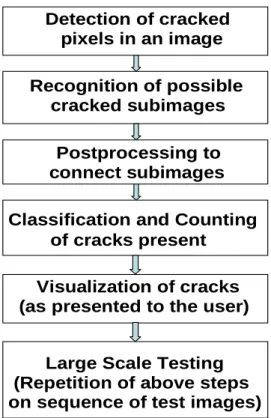
1.1 A Flowchart of the algorithm . . . 6

2.1 (a)Sealed Transverse crack (b)Unsealed Transverse crack . . . 11

2.2 A Code 0 transverse crack . . . 12

2.3 A Code 1 transverse crack, 1 4 inch with no roughness . . . 13

2.6 Another type of Code 3 transverse crack . . . 16

2.7 Longitudinal cracks . . . 17

2.8 Block cracks . . . 18

2.9 Fatigue/Alligator crack . . . 19

3.1 Original Image . . . 25

3.2 Thresholded Image . . . 26

3.3 Line detected Image . . . 27

4.1 Image after the recognition stage . . . 34

5.1 Image after Dilation . . . 37

5.2 Image after Erosion . . . 38

5.3 Image after Postprocessing . . . 40

(8)

6.2 Sealed subimage . . . 44

6.3 FFT of a subimage with a sealed crack . . . 44

6.4 Unsealed subimage . . . 45

6.5 FFT of a subimage with an unsealed crack . . . 46

6.6 Example of an unsealed Transverse crack . . . 49

6.7 (a) Thresholded Image (b) Line detected Image . . . 50

6.8 (a) Image after recognition (b) Postprocessed Image . . . 51

6.9 (a) Crack localization (b) Subimage profile . . . 52

6.10 (a) Example of a Longitudinal crack (b) Postprocessed Image . . . . 53

6.11 (a) Example of a Block crack (b) Postprocessed Image . . . 54

7.1 Left and right profiles of one pavement image . . . 58

7.2 Linear fit curves . . . 59

7.3 Filtered output using 5-foot Highpass filter . . . 61

7.8 Thresholded output of an 8-foot Highpass filter . . . 66

7.9 An example of application of wavelets to profiles . . . 67

7.10 Prediction error from application of RLS algorithm to profile data . 68 7.11 Prediction error from application IRLS algorithm to profile data . . 69

(9)

LIST OF TABLES

(10)

Chapter 1

Introduction

This chapter introduces the background, motivation and key contributions of the research presented in this thesis.

1.1 Background

Pavement distress analysis is one of the labor intensive tasks of Departments of Trans-portation (DOT) around the country. This is because, maintenance of ride quality for highway users includes determining pavement repair requirements in a timely fashion on a regular basis. Hence, DOTs across the country employ various strategies to diligently inspect sections of highways, collect information on pavement conditions and process it to extract meaningful data. Traditionally, manual inspection and data gathering has been the method of choice for detecting pavement damage. In such a system, trained experts walk or drive on highways that are to be inspected. Upon encountering a distress, the data is manually entered on a computer log. This process is not only cumbersome and time consuming but also involves a certain amount of risk, since the traffic flow on highways is hindered. In order to implement better data collection and processing, researchers migrated to automated analysis systems. Here, data collection is performed using specially equipped vehicles driving at highway

(11)

speed and recording information such as road profiles and pavement images. These are stored on high capacity computers to be retrieved and processed later. Yet again, manual intervention is required to assimilate road condition information by observ-ing the vast amount of data stored on the computers. Though risk free, this is still a tedious process. Hence, research is currently focussed on automating the process of analyzing stored data. Image processing has emerged as a popular tool in this pro-cess. With vehicles equipped with advanced camera and lighting systems, processing pavement images at highway speeds is now possible. The next phase of development involves analyzing these images and detecting pavement distress automatically.

Pavement distresses are a broad category of different anomalous phenomena occurring on pavements. These affect ride quality to different extents. Generally, distresses include cracking, patching and potholes, surface deformation (rutting and shoving), surface defects (bleeding, raveling and so on) and miscellaneous distresses. The Federal Highway Administration has published a Distress Identification Manual that lists the different types of distresses and the characteristics of each [1]. The primary focus of this thesis is on detecting cracking phenomenon and classifying its severity. The major types of cracks are transverse, longitudinal, block and fatigue. Further explanation on each of these is provided in chapter 2. In the next section, the prior research performed and the motivation behind the thesis are presented.

1.2 Motivation for this thesis

The necessity for automating the process of analyzing pavement condition data gen-erated by imaging vehicles cannot be overstated. Analysis of the large amount of data generated by the data collection system manually is impractical and time-consuming. In [2], cracks are manually detected on pavements and the suspect regions are pho-tographed. The images captured are then processed manually using a software to

(12)

segment cracked sections. It is evident that this process would be intractable for implementation on long sections of highways. Moreover, it would also be inconsistent due to operator errors. Hence, to eliminate such a tedious process and improve de-tection accuracy, researchers have focussed their efforts on effective image processing techniques to automatically detect cracks, with minimal or no human interaction.

Recently, Yamaguchi and Hashimoto proposed the use of improved percola-tion modeling as a technique to detect pavement cracks [3]. However, the process in [3] is not completely automated and may require human interaction to set certain seed parameters. From an image processing standpoint, there has been emphasis on pre-processing to remove noise while retaining already tested methods of crack detection [4]. The effectiveness of the proposed preprocessing technique was analyzed by testing 50 noisy concrete images. The authors in [4] mainly emphasize preprocessing with-out considering the variation in pavement roughness.Furthermore, the types of cracks present in the test images have not been provided. Hence, it is uncertain whether this system will perform optimally for all types and extents of cracks. In another paper, the Fast Haar wavelet transform is used to detect crack edges on concrete surfaces [5]. To improve the accuracy of the transform, ROC analysis is used to define the optimal parameter set, which includes the threshold for the edge detection algorithm. In [6], the authors propose the use of histogram projection to identify cracks within a cropped image. Histogram projection is the technique of averaging the pixel inten-sities in each row/column and smoothing the difference from a reference gray level. While [6] focussed on the severity of cracks, crack classification (in terms of sealed or unsealed), was not performed. Moreover, the system in [6] cannot detect multiple cracks within an image. In a research undertaken by the Texas Department of Trans-portation, pavement images were divided into grid cells of 8×8 pixels each, called seeds, and detection and classification were performed on the seeds [7]. A connection algorithm was used to cluster seeds in a linear string and thus detect transverse and

(13)

longitudinal cracks. Though this process is computationally not very complex, the performance may become poor for certain degrees of pavement roughness. For in-stance, on a rough surface, the contrast between the pixel intensities of a mild crack and neighboring background pixels may not be significant. In this case, the algorithm in [7] might not detect the crack. Thus, pixel intensity alone is not a robust feature for detecting cracks. In a paper by Bray [8], detection of cracks is performed using a neural network while classification is performed by another neural network. The proposed algorithm has not been tested on real images. The artificially generated im-ages may not yield a good picture of the computational complexity of the algorithm nor of the effectiveness of the technique on real images. Though there are some com-mercial software such as WiseCrax developed by Roadware Group Inc.[9] that can perform automated crack detection, their performance cannot be guaranteed. The results produced from these software do not meet the requirements of KDOT. For example, existing software solutions do not integrate profile data and image analysis, a feature that is desirable for quantifying the severity of cracks.

In [10], researchers at Utah State University (USU), in collaboration with the Utah Department of Transportation (UDOT), present a real time automated crack detection and classification system. Here, fuzzy logic has been used to de-tect distresses followed by a neural network that classifies the distress. It is well known that neural classifiers tend to perform poorly when test data deviates from training data. Therefore, the authors’ claim of high classifying accuracy is not well substantiated with a test set of just 42 images in [11]. Additionally, the sensitivity of the approach to variable operating conditions (for example, non-uniform lighting and varying pavement surface roughness) has not been analyzed. Neural networks have also been applied in [12] to classify pavement distresses. While the training data is artificially generated, the testing data comprises of both artificial and actual pavement images. However, the number of actual pavement images (83) is not large

(14)

enough for the conclusive evaluation of the technique. In [13] also neural networks are used to perform pavement distress detection and classification.

In a paper by Iyer and Sinha [14], image processing is used to segment cracking in underground pipes. Though this field of study is different from pavement analysis, the principles behind crack detection are identical. A contrast enhancement algorithm has been applied in this paper, followed by the application of morphology. The algorithms are adapted to account for pipe characteristics and appear to perform well. Hence, they may not be directly applicable to pavement images.

Therefore, a completely automated crack detection/classification system that can classify all types of cracks is still an open problem. For practical adop-tion of any new technology, the detecadop-tion system should be efficient, affordable and accurate. The research described in this thesis pertains to developing such a system for the Kansas Department of Transportation. Real pavement images were provided by KDOT. The algorithm developed using image processing and pattern recognition concepts is presented in the following chapters. The next section presents the key contributions of the thesis, while briefly introducing the steps in the algorithm.

1.3 Key Contributions

This section briefly describes the novel algorithm developed and the key contributions of the thesis.

The focus of this thesis is on developing a fully automated system that can read images stored in the database and process each image. The objective of this system is to detect and classify cracks in an image, presenting cracks localized within an image and discarding non-cracked images. Moreover, all types of cracks under different pavement roughness conditions are to be classified with high accuracy. Our proposed algorithm will reduce the labor involved in analyzing each image manually

(15)

Recognition of possible cracked subimages

Postprocessing to

connect subimages

Visualization of cracks (as presented to the user) Classification and Counting of cracks present

Detection of cracked

pixels in an image

Large Scale Testing

(Repetition of above steps on sequence of test images)

Figure 1.1: A Flowchart of the algorithm

and identifying images with cracks without the aid of any pattern recognition software. The proposed algorithm consists of four stages namely (1) detection; (2) recognition; (3) postprocessing, and (4) visualization. A flowchart indicating the sequence is shown in figure 1.1. The stages in this algorithm are explained in the following chapters.

Each test image is processed through the above stages sequentially and the final output image is presented to the end analyst along with the system’s observation on the cracked nature of the image.

The key contributions of the thesis are summarized below:

• The proposed algorithm is capable of detecting mild as well as severe transverse and longitudinal cracks.

• The detection stage, described in chapter 3, efficiently filters out most of the unconnected background noise and presents a more relevant image to the

(16)

suc-cessive stages.

• In the classification stage, pixels are grouped into subimages to reduce the com-plexity of further processing. The grouping process is presented in Section 4.1. The classification of subimages is validated using a Bayes classifier presented in Section 4.2. This stage performs further filtering of subimages that do not contain a significant percent of cracked pixels.

• In the recognition stage, the technique of Principal Component Analysis(PCA) has been applied to extract the weights associated with the cracked/non-cracked nature of a subimage. The extracted weights and the developed classifier work extremely well to distinguish between cracked and non-cracked subimages.

• Chapter 5 describes the postprocessing used to connect up cracked subimages that are not well connected and remove isolated subimages. Such cases of missing connectivity do occur frequently, especially in cracks that are mild. A final filtering process is applied to the image at this stage.

• Section 6.1, describes the metric used to automatically recognize a crack and localize it within an image. This metric works well to identify the region in which a crack is present. Even multiple cracks within an image are located accurately in this stage.

• Once the region of the crack has been identified, the crack is further classified as sealed or unsealed, in the case of transverse cracks. This classification is important to analysts since the need for repair is determined based on whether the crack has already been attended to by way of sealing. Further information on sealing of cracks is presented in Section 6.2.

(17)

images before running them through the whole process so that the algorithm is again presented with cracks running in the transverse direction.

• When tested on a large set of real pavement images, the algorithm is found to have a detection probability of 97.10% for transverse cracks and 94.11% for longitudinal cracks.

• The most important contribution of the thesis is that the developed algorithm is completely automated. The thresholds used are adaptive. Hence, there is no need for human interaction till the whole data set has been processed and the results stored.

To summarize, our algorithm automates the process of crack detection and classification from real pavement images. It can be applied on transverse and longi-tudinal cracks with a high rate of detection and very low rate of false detection.

1.4 Organization of the thesis

The rest of the thesis is organized as follows : Chapter 2 introduces the classifications of cracking phenomena and the data collection equipment installed in the imaging vehicle; Chapter 3 describes the stage of preprocessing/detection of cracked pixels from an image; Chapter 4 deals with the core recognition process, where subimage level classification is performed; Chapter 5 deals with postprocessing of the image, i.e., the application of morphology to connect cracked subimages and remove isolated subimages; Chapter 6 describes image level classification, sub-classification of cracks present, counting them and presenting the information to the end user for easy vi-sualization, along with large-scale testing results; Chapter 7 presents a discussion on profile data and their significance, with a description of the techniques being con-sidered to analyze them; finally, Chapter 8 presents the conclusion of the thesis, a summary of its key contributions and future research extensions.

(18)

1.5 Summary

This chapter presented the background of the research, the prior work done, the motivation for the thesis and its key contributions. In the next chapter, the reader is introduced to different crack classifications and the data collection system.

(19)

Chapter 2

Pavement Distress Phenomena

In this chapter, we present the classifications and sub-categories of pavement cracking and the measuring system used to collect pavement images. Image examples for each type of cracking are presented, along with their primary features. Classi-fication of cracks depends on their alignment and structure. Hence, these are the features that have to be intelligently extracted by the algorithm to perform accurate classification. A study of such features aids in the development of an automated clas-sifier. A brief explanation of some of the main characteristics of cracks are presented in this chapter. In Section 2.3, the data collection vehicle is presented. A brief dis-cussion of manual recording of pavement distresses by visual inspection is presented to enforce the necessity of automation. The performance of the measuring system is of utmost importance to pavement maintenance. This is because inaccurate data collection could introduce artifacts into the images captured, which lead to increased complexities of processing algorithms.

2.1 Transverse cracking

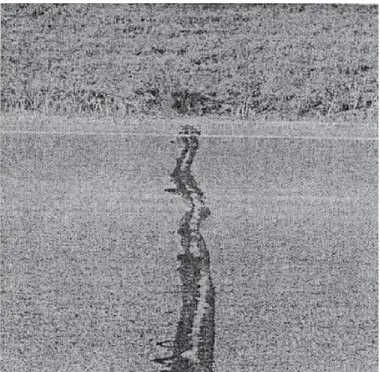
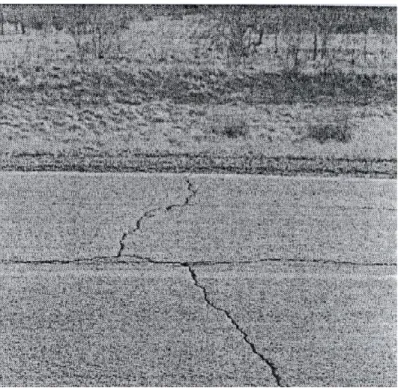
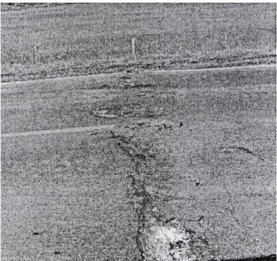
Transverse cracks are cracks that run across the width of the pavement surface, i.e., from left to right. Examples of transverse cracks are shown in figure 2.1.

(20)

(a) (b)

Figure 2.1: (a)Sealed Transverse crack (b)Unsealed Transverse crack

One type of classification of Transverse cracks is based on whether they are sealed or unsealed. Sealed cracks are the ones to which a sealant has been applied in order to control its growth. Further reasons for using sealing as a method of countering cracks can be found in [15]. Hence, this classification indicates to the end user the status of a crack,that is, if it has been already treated or if it requires repair. Some examples of transverse cracks are presented in figure 2.1.

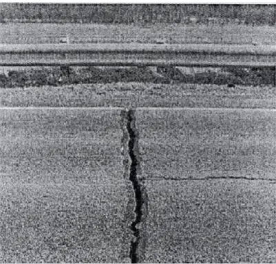
Another way of classifying Transverse cracks is based on severity, which is measured in terms of crack roughness. Roughness of a crack, quantified in terms of the International Roughness Index (IRI), indicates the deviation from a perfectly planar surface [16]. The lower the IRI, the less rough a crack is. In turn, the less it affects ride quality and vehicle dynamics. The classification based on roughness identifies transverse cracks as Code 0,1,2 or 3 cracks.

(21)

Figure 2.2: A Code 0 transverse crack

• Code 0 cracks are defined as mild cracks that are sealed but have no roughness or break in the sealants. A code 0 crack is represented in figure 2.2.

• Code 1 cracks are sealed/unsealed and with no roughness as shown in figure 2.3.

• Code 2 cracks are sealed/unsealed with noticeable roughness with no depression and of width greater than one inch. Figure 2.4 presents a code 2 transverse crack.

• Code 3 cracks are sealed/unsealed with significant roughness caused by extreme depression. There is also secondary cracking associated with the crack. A Code 3 crack is presented in figure 2.5. Figure 2.6 represents another type of code 3 cracking.

(22)

Figure 2.3: A Code 1 transverse crack, 1

4 inch with no roughness

The descriptions of the coded cracks and the images of each type of cracking shown above have been provided by KDOT [17]. The primary focus of this thesis is on transverse cracks which occur more commonly than other types of cracks. The high frequency of occurrence of transverse cracks also provides large training data that can be utilized to condition the detection algorithm effectively. Moreover, the set of training data comprised of pavement surfaces of different degrees of roughness. Hence, wide variations in the pavement roughness have been accounted for in the algorithm. In the next section, we present a brief description of the other types of cracking which, though not frequent, still occur.

(23)

2.2 Other cracking phenomena

In this section, we present the characteristics of other types of cracks that occur on pavement surfaces.

2.2.1 Longitudinal cracks

Longitudinal cracks, as the name implies, run along the length of the pavement sur-face, i.e., in the direction of travel on roads. In other words, longitudinal cracks are perpendicular to transverse cracks. This alignment of longitudinal cracks can be ex-ploited to detect them. Since images are processed by treating them as matrices, a transposed longitudinal crack can be presented as a transverse crack to the detection algorithm. This operation adapts the image for processing by the same algorithm and the rate of detection could be expected to be as accurate as for actual transverse

(24)

cracks. Examples of longitudinal cracks are indicated in figure 2.7. The requirement for a longitudinal crack to be considered significant is that it should lie in the wheel path, i.e., the portion of the pavement where the wheels of vehicles predominantly travel.

2.2.2 Block cracks

Block cracks comprise of rectangular blocks of interconnected transverse and longi-tudinal cracks. For example, the images presented in figure 2.8 indicate typical block cracking (courtesy : Google images).

The detection of such cracks can be achieved using the algorithm presented in the thesis easily enough. Whereas, the classification requires identifying the fact that the cracks present are interconnected. This might require some additional loop

(25)

Figure 2.6: Another type of Code 3 transverse crack

detecting algorithms or the presence of multiple transverse and longitudinal cracks can be assumed to represent a block crack.

2.2.3 Fatigue cracks

Fatigue cracks, also known as Alligator cracks are very finely developed patterns that appear as secondary cracking stemming from longitudinal/transverse cracking. These occur as a result of excessive loading and a weakening of the structure beneath the surface. Hence, the cracking described earlier are predominantly surface phenom-ena while fatigue cracks indicate the beginning of structural damage. Such cracks comprise of finely interconnected web-like cracking that resemble an alligator’s hide. Hence the name alligator crack is associated with this type of cracking. Examples of fatigue cracking are presented in figure 2.9. These cracks differ from block cracks

(26)

(a) (b)

Figure 2.7: Longitudinal cracks

because of the higher fineness of interconnection.

In order to detect fatigue cracking, the processing must be done at lower resolutions. That is, while considering features within subimages of a test image, the size of the subimages may have to be as small as 8 ×8 pixels, while a larger size of 32×32 pixels has been determined to be appropriate in the developed algorithm for detecting transverse and longitudinal cracking. Since, the fine cracks are also interconnected, again loop-detection algorithms might accurately detect and classify such cracks.

In the following section, the data collection vehicle and the associated equip-ment are presented. A brief description of the technique used by KDOT to record observations on cracking types and the location of cracks on highways is also pre-sented.

(27)

Figure 2.8: Block cracks

2.3 Measurement system

In this section, we present the measurement system and techniques that have been used by KDOT to generate images of pavements and the left and right profile data for each image. Longitudinal profile data or height profiles of cracks indicate the amount of structural damage related to the crack [18]. These are applied in determining the roughness characteristics of the pavement and hence the effect on ride quality.

2.3.1 The Data collection vehicle

In this section, the data collection vehicle driven along highways to capture pavement images and profile data is briefly introduced [19].

An International Cybernetics Corporation(ICC) imaging vehicle that col-lects real-time high-resolution digital pavement images in all lighting conditions is

(28)

Figure 2.9: Fatigue/Alligator crack

used to map pavements at driving speeds. Quality images can be collected at speeds up to 70 mph. The vehicles consist of (1) a pavement camera(downward) system, (2) rack mounted computers, (3) laser sensors, (4) pavement lighting systems, and (5) Global Positioning System. The forward cameras, focussing on the pavement in front of the vehicle, are DVC-1310c digital video cameras with a progressively scanned im-age format. The downward cameras, mounted in the rear and focussing down on the road surface, are high performance, high-resolution Basler L103 line-scan cameras. Sign cameras are focussed on the side of the road for right of way analysis. The forward and line scan camera computers comprise of 3.0 GHz Pentium IV processors working on Windows 2000 with additional software that synchronize the cameras and lighting. The lighting system consists of ten 150 Watt lamps, each of which has a polished reflector designed for efficient operation. Laser sensors located on the front

(29)

bumper record the pavement elevation data, generating pavement profiles. The image data recorded using this system is saved on removable hard drives for further analysis. The information about the data collection equipment was provided by KDOT [20].

The data collection system plays an important role in this application since factors such as lighting on the pavement, position of the cameras and so on affect the quality of images used in further processing. Artificially introduced artifacts such as non-uniform lighting in images are some of the effects that have to be accounted for by image processing algorithms. Hence, the more accurate the data collection, the less complex the processing algorithms have to be.

2.3.2 Recording of crack classification

The technique currently used by KDOT to classify observed cracks on highways is based on the decision of an expert. An operator on the vehicle controls the processing of the camera-computer system. Every time a crack is observed in the image of the current section of highway, it is classified visually and the observation is recorded on a computer log. Hence, the vehicle is driven at speeds lower than highway speeds near the shoulder of the lane. This method of data recording could lead to inconsistent classification since a vast amount of data is processed very quickly. The decisions can be expected to be strife with human errors that tend to occur. Instead, if an automatic detection and classification system is implemented, the stored images could be processed in real-time or off line without human intervention. Such a system would avoid inconsistencies and save manual labor.

At present, though, pre-classified images and the profile data are provided for this research. The decision of the algorithm is compared with expert decisions to determine the accuracy of the algorithm. In later chapters, we present findings on the performance of the algorithm, which is found to be extremely accurate for transverse cracks.

(30)

2.4 Summary

In this chapter, we described the types of cracking generally observed on pavements, along with image examples. We also made observations on key features of each type of cracking that can be exploited to detect and classify them. In the final section, we presented a description of the data collection vehicle utilized by KDOT to capture pavement condition data. The technique of manual observation and classification is explained in Section 2.3. In the next Chapter, we present the first stage of the algorithm, i.e., the detection/preprocessing of pixels. This stage classifies pixels as cracked/non-cracked and filters out the pixels that are unconnected to other cracked pixels.

(31)

Chapter 3

Detection/preprocessing of cracked

pixels

This chapter deals with the detection of cracks that appear in the pavement images. Pixel-level classification is performed in this stage, i.e., pixels are classified as cracked/non-cracked. The stages of preprocessing used to remove noise from the pavement image and detect connected sets of pixels that persist after noise removal are described in this chapter. We begin by presenting a brief introduction to images and how they are processed.

3.1 A brief introduction to the world of pixels and images

An image is a 2−D digital representation of a scene captured from light reflecting off of the subject. The smallest unit of an image is the picture element or pixel [21]. A pixel can be thought of as a uniform square containing some definite value of intensity or color. A number of pixels are assembled together like the pieces of a jigsaw puzzle to create a whole image. The resolution of the image is commonly such that, individual pixels are not visible as discrete squares but the complete image contains smooth gradients of color intensities. When there are objects within an image with

(32)

sudden change in pixel values from the neighboring pixels, these appear as edges. Image processing is a vast field with applications in various areas such as transportation, medicine, military surveillance and so on. It involves extracting mean-ingful information from images by applying certain processes to them [22]. Though a lot of techniques are generic, some algorithms are customized depending on the application and the type of images that have to be processed. Image processing is, in fact, a branch of signal processing in which the input is an image. A detailed discussion on image processing algorithms can be found in [23].

Pavement images consist of a smooth consistent background. When cracks are present, these appear as a string of lower intensity pixels (darker than the pave-ment surface). Hence, the main characteristic of cracks exploited to detect them is their lower pixel intensities compared to the background pixels. In our algorithm, this feature is used in the preliminary step of thresholding as described in the following section.

Throughout this discussion, the size of the images are uniform and are 3344×

2048 pixels (6.44m×3.94m). Each pixel is 1.93mm×1.93mm in the images. The size of the images becomes relevant when computational complexity of processing them is to be considered.

3.2 Steps involved in the detection of pixels

The processes used to achieve noise reduction and detection of connected pixels are:

Thresholding

Thresholding has been used widely as a basic technique for segmentation of the fore-ground from the backfore-ground, noise removal, as well as image equalization [24] [25]. Generally, setting the threshold is a vital step before further processing since, using

(33)

appropriate thresholds, the noise from the image can be reduced to a great extent. In our process, thresholding is used to classify pixels as cracked or non-cracked. Here, the local statistics, i.e., mean and variance along every column and sets of rows from the image, taken one at a time, are determined. Each pixel within this block of few rows and all columns is classified as cracked/non-cracked based on a threshold corresponding to

T =µ−σ (3.1)

where µ is the local mean and σ is the local standard deviation. Denoting the pixel value at location (x, y) in the image asp(x, y),

p(x, y) =      1 cracked if p(x, y)< T 0 non-cracked if p(x, y)> T . (3.2)

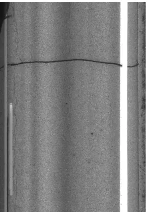
Here is where the typical characteristic of cracked pixels having lower intensities than the background is utilized. The motivation for using a block statistic is to overcome any localized image artifact. Thus, an adaptive thresholding technique is used as the first stage of crack identification. As a result, the problem of misclassification with a single global threshold set for an entire image is avoided as well. An image with a sealed transverse crack is shown in Figure 3.1 and the result of thresholding it is shown in Figure 3.2.

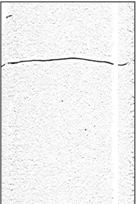
In figure 3.2, a light band is seen around the crack, the cause of which is explained as follows. The processing and rendering of the image in the document cause a variety of image artifacts. When viewed on a display, the background area away from the crack, consists of highly uncorrelated pixels without an organized pattern. In the rendered image, many of the pixels coming through the threshold appear to be touching but in reality they are not. Another effect that appears in the rendered image is the light band around the crack. This band is caused by the adaptive threshold applied to the image, and is not a rendering effect. As the algorithm gets near the

(34)

Original Sealed Transverse Crack

Figure 3.1: Original Image

crack the low pixel values of the crack pixels drive the threshold lower, causing fewer pixels to come through, thus creating the light band seen in the image.

3.2.1 Line Detection

Line detection denotes the process of searching for connected pixels that represent lines in the image within a certain range in the horizontal, vertical and diagonal directions. Since cracks consist of short linear segments, this range is fixed as 5 pixels, a small fraction of the subimage length to be used later in the recognition process. This process eliminates much of the clutter that resulted from thresholding the image. The larger the range within which connected sections are searched for,

(35)

Thresholded Image

Figure 3.2: Thresholded Image

connected segments, larger ranges could miss these cracked portions. Hence a tradeoff is required to find the optimal range. We determined that choosing 5 pixels was appropriate to preserve maximum possible information about the cracked portions in the image. The process of searching for connected pixels is repeated in the horizontal, vertical and diagonal directions for each cracked pixel. This accounts for all possible directions in which a crack could extend. Upon line detection the thresholded image in Figure 3.2 is transformed as shown in Figure 3.3.

From Figure 3.3, it is observed that the process of line detection causes a filtering effect by retaining only connected pixels. Hence, the number of noisy pixels is reduced in the image after line detection. There are, however, a large number of noisy pixels which need to be filtered out to avoid false detection in the final stages

(36)

Line detected image

Figure 3.3: Line detected Image

of the algorithm.

3.3 Summary

In this chapter, we have described the basic preprocessing performed on an image to remove most of the background noise and preserve only the connected cracked pixels. The efficiency of this stage is critical to the subsequent stages since the presence of a large amount of clutter would affect the higher levels of classification. It is noteworthy that the pixel detection algorithm presented in this chapter works very well to attain the objective of determining cracked pixels that are connected to other cracked pixels. The next chapter presents the stage of subimage level classification used to further

(37)

(38)

Chapter 4

Recognition of cracked subimages

This chapter deals with classification at the subimage level, i.e., recognition or validation of the subimages that contain some portion of cracked pixels. In this stage, the image is divided into subimages of size 32×32 pixels. This division reduces the complexity of further processing. The size of the subimage is chosen such that it sufficiently characterizes the complete crack as well as reducing processing time. The steps involved in classifying the subimages and the basic concepts that have been applied are presented in the following sections.

4.1 Grouping of cracked pixels

The classified pixels are grouped into subimages of size 32×32. Next, each subimage is classified as cracked or non-cracked based on the number of cracked pixels in it. We set our decision threshold to 10%, i.e., if 10% or more of the pixels in a subimage are cracked, the subimage is classified as cracked. The purpose of grouping is to restrict all further processing to the subimages so as to reduce computational com-plexity. Furthermore, when characterizing cracks as sealed/unsealed (Section 6.2), this characterization is made based on classification of subimages as sealed/unsealed. Therefore, only by grouping pixels into subimages can this classification be performed

(39)

at the subimage level. Grouping pixels into subimages has been applied previously in [26]. In this paper, though, the subimage size used was 64×64 pixels. The high rate of false object detection (0.79) per image frame indicates that the algorithm is not very efficient. It is observed that the subimage size of 32×32 sufficiently captures cracking information from the image. A smaller size, such as 8×8, leads to slower processing, which can be avoided when there is no fine cracking. A larger size was found unsuitable since portions of cracks were incompletely traced, thereby causing loss of data.

4.2 Recognition using Principal Component Analysis(PCA)

In this section, we present a discussion of the technique used to extract features that can distinguish cracked and non-cracked images. A brief explanation of PCA is provided and its application to pavement cracking is substantiated with image results.

4.2.1 Principal Component Analysis

In the recognition phase of the algorithm, the 32×32 subimage classification is further refined using PCA based feature extraction. PCA is a statistical technique used to reduce the dimensionality of data. The principal components extracted from a given data set are determined such that they represent as much of the variation in the data as possible without considering all the points in the set. A description of this technique is found in [27]. In [28], the authors propose the application of PCA to enhance open cracks that occur on severe metallic surfaces. PCA has been used for thermal effect enhancement while processing thermographical images of metallic surfaces for open cracks. This is one possible application of PCA, which is a very commonly used effective data processing technique. In our application, we propose the use of PCA to extract principal features that could distinguish cracked sections

(40)

of an image from non-cracked sections.

4.2.2 Application of PCA on images

PCA is initially performed on a set of 50 concatenated non-cracked images, and three basis vectors corresponding to the first three principal components are extracted. The first three components constitute our feature set as they capture around 96−

97% of the information in an image and can be used to adequately characterize the entire image. Following the extraction process, we populate two training classes of cracked and non-cracked subimages from 50 cracked and non-cracked images. Each cracked subimage is projected onto the basis vectors and three weights,w1, w2 andw3, are extracted. These weights indicate the amount of energy present in each of the principal component directions in the vector space defined by the basis vectors. This process is repeated for all the collected cracked subimages. Simultaneously, the same process is performed on the collection of non-cracked subimages as well to obtain weights for the class of non-cracked images. The number of subimages in each class is increased by testing more images and hence, more weights are appended to the classes. There are six distributions of weights totally, and each can be characterized using the probability density functions. As per central limit theorem, the weight distributions are observed to be normal with different means and variances [29]. In order to test a subimage for the presence of a crack, its three weights, wi, i= 1,2,3, are obtained

by projecting the mean subtracted subimage onto the bases vectors computed earlier. Each of these three weights are compared to two distributions - wc,i distribution for

the cracked class and wuc,i for the non-cracked class. The probability of the test

subimage weights being closer to one distribution than the other is computed as a likelihood function presented in equation 4.2. This likelihood function is compared to a threshold as shown in equation 4.4 based on which the subimage is classified. Thus, a Bayes likelihood test, with the following hypotheses, is developed under the

(41)

assumption of normality [30].

Cracked H0 : wi ∼N(µc,i, σc,i2 ) i= 1,2,3

Non−cracked H1 : wi ∼N(µnc,i, σnc,i2 ) i= 1,2,3 (4.1)

where µc,i and σc,i are the mean and variance of weight wc,i for the class of cracked

subimages; µnc,i and σ2nc,i are the mean and variance of the weightwnc,i for the class

of non-cracked subimages. The likelihood ratio based on weight wi is formulated as

L(wi) = 0.5 log σ2 c,i σ2 nc,i +(wi −µc,i) 2 2σ2 c,i − (wi−µnc,i) 2 2σ2 nc,i (4.2) where i= 1,2,3. Assuming a uniform cost function and defining the thresholdτ as

τ = Pc Pnc

, (4.3)

where Pc and Pnc are the prior probabilities of a subimage being cracked or

non-cracked respectively, the Bayes test is given by

δ(wi) =      1 L(wi)> τ 0 L(wi)≤τ . (4.4)

Thus a value of 1 for δ(wi) indicates a cracked subimage while 0 indicates

a non-cracked subimage. The prior probabilities Pc and Pnc are evaluated based on

existing data on pavement distress. In our analysis, we determine that Pc = 0.0435

and Pnc = 0.9565.

4.2.3 Decision via sensor fusion

The decisions based on the three weights i.e. the results of the Bayes test for i = 1,2 and 3 are fused using the OR rule and a combined decision is used to classify the subimage. Thus, a sensor fusion like approach is applied to validate the decision of the classifier. Sensor fusion is a technique applied to enhance the reliability of the

(42)

output or decision of one sensor. Decisions reported by multiple sensors which work independently can be fused to make the result more accurate than the output of one sensor [31]. In this research, the decisions of the classifier based on each of the three weight features are treated as independent sensor decisions and fused so as to obtain a better classification of subimages. It is visually observed that this type of fusion results in a nearly complete crack compared to when one of the weights is used. In the latter case, a lot of cracked subimages get filtered and the crack appears incomplete in parts.

4.3 Image results

The image obtained after recognition is presented in figure 4.1.

Blocks of size 32×32 are observed to constitute the crack in the recognized image. The number of classified subimages is much lower than what was detected. Thus, noise reduction occurs in this stage as well. It is evident from the image that, the chosen subimage size is appropriate for characterizing cracks present. This claim is further substantiated in Section 6.4 by presenting an example of an unsealed crack that has been processed.

4.4 Summary

In this section, the process of grouping pixels into subimages to reduce computational complexity has been presented. We also describe Principal Component Analysis as applied in feature extraction for distinguishing cracked and non-cracked images. Fol-lowing this section, a brief discussion on classification of subimages via sensor fusion is presented. Finally, the image resulting from the application of PCA based recog-nition is shown and observations are presented. In the next chapter, postprocessing performed on the recognized images is described.

(43)

after recognition

(44)

Chapter 5

Postprocessing

In the previous chapter, the third stage of the algorithm, i.e., recognition of subimages, was presented. The image after recognition is comprised of square blocks or subimages. For any cracks present, subimages constituting the cracks are clearly observed. There are certain cases of mild cracking in which the cracked subimages are not completely connected. Moreover, there are cases of isolated non-cracked subim-ages throughout the image as observed in the figure presented in Section 4.3. Hence, postprocessing is performed on the recognized image to establish subimage connec-tivity and filter out isolated subimages. This stage is comprised of two processes : application of mathematical morphology and filtering.

5.1 Mathematical Morphology

Morphology, or the science of shape, has been applied in image processing very ex-tensively. Specifically, this technique has been applied in areas such as image en-hancement, feature extraction and object recognition [32] [33]. With primary focus on binary images, morphology deals with representing objects in an image in more useful forms. A variety of filtering effects can be created from combinations of dif-ferent morphological operations. In simple terms, morphology involves filtering an

(45)

image with a suitable structural element that is sequentially placed over every pixel in the image. Structural elements can be linear, circular or any other shape depend-ing on the objects to be recognized or enhanced. In [34], the authors have applied morphology as part of an image processing algorithm to detect cracks. Several other similar research efforts have included morphology as the final stage before presenting the resultant image to the end user. This extensive usage of morphology indicates its effectiveness in relevant applications. Since pavement distress detection can be treated as an image enhancement problem, morphology can be applied to cracked images to efficiently segment the cracks and eliminate clutter and pavement noise.

There are two basic morphological operations, namely dilation and erosion, that can be employed to enhance the objects in an image. Dilation is the process of removing small holes while erosion is the process of removing small objects. Image di-lation causes subimages to get elongated and hence connection is established between subimages that are not adjacent but are part of the same crack. Then, by eroding this image, objects are compressed to their original size but the previously established connection is maintained. A closing operation (dilation followed by erosion) is thus used to enhance the objects in the image, i.e., distresses such as cracks in this case. As expected, it is observed that slight cracks appear better connected after the ap-plication of the above processes. Furthermore, a large number of isolated subimages that were retained till this stage are removed from the image by the application of morphological closing.

The choice of the structural element is an important factor to be considered while dilating or eroding an image because the shape of the objects in the image could get distorted by the application of the wrong type of structuring element. Since pavement cracks are made up of linear segments, linear structuring elements are used to perform a closing operation on the image. A 4-pixel wide horizontal line filter is used to close the image. In parallel, another line filter, vertical and 4 pixels

(46)

long, is applied to detect any longitudinal aberrations in the image. Once again, the choice of pixel length was based on our experience from analyzing actual images by applying morphology. When the pixel length is set at 3 or lower, connectivity is lost in several sections of a crack. On the other hand, for a pixel length of 5 or greater, several isolated non-cracked subimages were artificially connected, presenting false information. The pixel length of 4 connects up adjacent cracked subimages well enough for a crack to be recognized while avoiding spurious connections between isolated subimages.

The image that results upon dilation of the original image is presented in Figure 5.1 and the result of erosion on the dilated image is shown in Figure 5.2.

Re−sized dilated image

Figure 5.1: Image after Dilation

Generally, morphological operations are applied at the pixel level. Moreover, for large images, the operations tend to become computationally very intense. Hence,

(47)

Re−sized eroded image

Figure 5.2: Image after Erosion

result, the size of the image used in this stage is 105×64 pixels. After postprocessing the image, it is again re-sized to its original dimensions. Following morphology, a final filter is applied to the image to remove isolated subimages. The design of this filter is presented in the following section.

5.2 Filtering

The postprocessed image consists of fewer isolated subimages than the image imme-diately after recognition. The persistence of such subimages is due to clustered sets of non-cracked subimages consisting of some anomalous surface phenomenon which might have been detected as a crack. In spite of the reduction in the number of falsely detected subimages, a more precise image is desired in order to avoid false localiza-tion of cracks within the whole image. Hence, a final filtering process is performed

(48)

on the image. The design of this filter is based on the simple idea that any detected subimage that is not surrounded by any other detected subimage within a certain radius in all directions around it is considered isolated enough to be eliminated. The radius is heuristically determined to be thrice the length of a subimage and it has been found to perform well in eliminating isolated subimages.

5.3 Image results

Upon postprocessing, the resulting image appears as shown in Figure 5.3. As observed in the image, there are very few isolated subimages that are retained after postpro-cessing. However, even a few subimages that are oriented across a single row could affect the detection of a cracked row in the next stage where the cracked subimage count is used to classify the whole image as cracked or non-cracked. This problem is explained further in Section 6.1.

5.4 Summary

In this chapter, we presented the stage of postprocessing applied to the image after recognition of the cracked subimages. Most of the isolated subimages were efficiently eliminated while connectivity is established between subimages constituting the actual crack. The final filtering process further reduced the remaining isolated subimages in order to avoid false crack localization in the next stage of image level classification. In the next chapter, the feature used to identify the precise locations of cracks within the image is presented. In addition, the performance of this feature in classifying whole images is indicated. Also presented in this chapter is the application of a Fourier based technique to classify cracks as sealed or unsealed, which determines maintenance requirements for the cracks.

(49)

After postprocessing

(50)

Chapter 6

Image classification, crack

counting, visualization and

large-scale testing results

In the previous chapter, we described the third stage in the algorithm, i.e., postprocessing performed to establish connectivity among cracked subimages and to eliminate isolated noncracked subimages. In this chapter, the algorithm progresses to image level classification. In this stage, the number and orientation of cracked subimages are exploited. These characteristics are used to classify the whole image as cracked or noncracked. Furthermore, the exact locations of cracks within the image are identified and highlighted for better visualization. As a result, the number of cracks present is also determined automatically by the algorithm. The most important contribution of this stage is the sub-classification of cracks as sealed or unsealed using a Fourier transform based approach. Further explanation on this nature of the subimage and its significance is provided in Section 6.2. In closing, large-scale testing conducted on the complete algorithm is presented. The results observed along with the probabilities of detection and false alarms are presented to validate the

(51)

performance of the algorithm.

6.1 Image classification

0 10 20 30 40 50 0 500 1000 1500 2000 2500 3000 3500

Figure 6.1: Original image with its subimage profile

In order to localize the cracks within an image, the number of cracked subim-ages per row and per column are determined and plotted. The subimage profile de-veloped for the transverse crack under consideration is shown in figure 6.1. In the plot shown, the y− axis represents the row number and x− axis represents the subimage count. This count of cracked subimages is termed as subimage profile, not to be confused with pavement profiles that indicate elevation nature of pave-ments. The steep increase in the subimage profile in the plots indicates the presence of cracks. This feature can be exploited to further localize the crack and present it to the user. Comparing this count to the average score of the image with a tolerance

(52)

of 2×standard deviation indicates the location of the crack. By considering either the whole image or subbands of the image, multiple cracks, in either direction, can be detected. By tracking the number of occurrences of the subimage profile exceed-ing the threshold, the total number of cracks that occur in an image is determined. Hence, this level of classification is of very low complexity from a computation stand-point. The importance of presenting a clutter free image to this stage should be noted. When there are falsely detected subimages present, they shift the statistics of the subimage profile. As a result, the rows around which these false alarms occur could also be identified as containing parts of cracks leading to false classification. Hence, the number of isolated noncracked subimages needs to be restricted before this stage. A few cases of isolated subimages do not affect the threshold greatly since it is dominated by actual cracked subimages which exceed isolated subimages signif-icantly. The feature of subimage profile is observed to detect cracked rows/columns within images highly efficiently. Hence, the classification of whole images is accurate as well.

From a visualization standpoint, the ability to highlight a crack is useful for the end analyst. Therefore, while displaying the images we have consciously represented the cracks against a white background. Integrating the location of cracks with a mapping software can provide valuable information for maintenance activities.

6.2 Classifying sealed and unsealed cracks

When a region within an image is determined to contain a crack, the cracked subim-ages in this region are tested to determine if the crack is sealed or unsealed. Sealed cracks are those cracks to which sealants have been applied so as to control the rate of their growth and the pavement roughness caused by serious cracking. Hence, sealed cracks do not represent an immediate threat to pavement health whereas unsealed

(53)

cracks, specifically ones that extend across the width of the pavement require atten-tion.

Figure 6.2: Sealed subimage

Stacked fft of a cracked subimage

column no −−−−> row no −−−−> 5 10 15 20 25 30 5 10 15 20 25 30

Figure 6.3: FFT of a subimage with a sealed crack

The application of sealants makes cracks wider than unsealed cracks, also making them very distinct and easier to detect. From visual observation of samples of both types of cracks, it is intuitive that the frequency response of each must be different. This is to be expected since a sealed crack is very distinct from the pavement surface and hence there is a large intensity gradient at the crack edges. In comparison, there is little or no distinction between unsealed cracks and the pavement surface. Hence the frequency response of unsealed cracks are expected to resemble that of the

(54)

noncracked pavement more closely than the response of sealed cracks. Therefore, the frequency characteristic of a crack is a possible measure of classifying it. To extract the frequency content of subimages, we perform 2−DFourier transform on them. The FFT of various 8×8 portions of each test subimage are computed and their magnitudes are stacked. The frequency response resulting from the stacking has a distinct shape indicating the orientation of the crack within the subimage. This technique of stacking up the magnitudes of the FFTs has been previously applied [35] to analyze quality of baked products. The stacked magnitudes of the frequency responses have an expected value which is a scaled version of the frequency response of the subimage. This has been proven mathematically in [35]. If the Fourier transform of the 32×32 subimage is represented as S32×32 and that of the 8×8 subimage as S8×8,

E{|S8×8(x, y)|2}=|S32×32(x, y)|2N (6.1) where N is the number of 8×8 subimages within one 32×32 subimage.

Figure 6.4: Unsealed subimage

Equation 6.1 indicates that the summed magnitudes of FFTs from identical 8×8 portions of a subimage serve to emphasize the dominant features in the subimage representing a crack.

(55)

Stacked FFT of an unsealed crack 5 10 15 20 25 30 5 10 15 20 25 30

Figure 6.5: FFT of a subimage with an unsealed crack

visualization, a larger area has been presented. Figures 6.3 and 6.5 present the image representation of the Fourier transform of a subimage from the sealed and unsealed cracks respectively. From figure 6.3, it is seen that sealed cracks exhibit a narrow response while unsealed cracks have a greater spread in their response. A measure that characterizes the spread can serve as the feature to distinguish between sealed and unsealed cracks. Specifically, the number of significant frequency components, Kwf, in the spatial domain is used as an indication of the spread in the FFT. In

practice, frequencies having magnitudes greater than 20% of the maximum frequency are considered significant in the frequency response of a subimage. Computing this feature for a large number of subimages yields a normal distribution for each class with different means and identical variances, i.e., N(µsealed, σs2) and N(µunsealed, σ2s). For a test subimage, the number of significant frequency components are determined and compared to the means of the two classes. The resulting decision is similar to the Gaussian location testing rule and can be represented as

δ(Kwf) =     

sealed d(Kwf, µsealed)<d(Kwf, µunsealed)

unsealed d(Kwf, µunsealed)<d(Kwf, µsealed)

. (6.2)

where d indicates the distance between the metric and the means of the distributions. All the subimages within a detected region in the image are subjected to this test. If

(56)

the majority of the subimages are classified as sealed, the crack as a whole is classified as sealed. On the other hand, the crack is classified as unsealed if the majority of the subimages are classified as unsealed. With 50 test images, the proposed technique provided 100% accurate classification of sealed and unsealed cracks.

6.3 Large scale tests

• The term ’large scale’ is used to indicate that a sequence of images have been processed sequentially by the algorithm which retrieves images automatically from the database. A set of 1000 images that contain transverse cracks ranging from severe to mild have been processed by the algorithm. This set also consists of some noncracked images. It is observed that the algorithm has a high rate of crack detection with a low false alarm rate. Specifically, the probability of detection of cracks is found to be 0.9710 and the probability of false alarm is found to be 0.0076. One key observation is that even multiple cracks within an image are detected accurately. However, in some cases of mild cracks that do not run across the width of the image, there is a possibility that the crack goes undetected. But, as is evident from the remarkably high rate of detection, such occurrences are rare.

• As far as longitudinal cracks are concerned, around 34 images containing longi-tudinal cracks were tested. The probability of detection was found to be 0.9411. However, there were more false alarms compared to transverse crack testing. A higher false alarm rate of 0.20 is induced by artifacts such as lightning stripes and surface characteristics. Distinguishing such clutter from relevant cracking will require a more complicated detection algorithm as compared to transverse crack detection.

(57)

might be interpreted as non-cracked portions in the image. The large set of im-ages contains pavements with different types of surfaces, with varying degrees of texture. The more texture the pavement surface has, the more chances of misclassification since slight cracks are difficult to distinguish from such back-grounds.

• The accuracy of sealed-unsealed crack classification is found to be 100% in the 50 test images considered. There is a small probability of misclassifying non-cracked images as sealed images when there is non-uniform lighting, such as shadows or dark stripes in the image. Also, some sealed cracks that are thin may get misclassified as unsealed cracking. But the probability of these occurrences is expected to be tolerable.

6.4 Image Examples

An example of an unsealed transverse crack is shown in figure 6.6. The results of applying the detection algorithm on this image are indicated in figures 6.7, 6.8 and 6.9. It is observed that despite the crack appearing to be slight against the pavement surface, the algorithm detects and localizes it accurately indicating the algorithm’s robustness.

Examples of images containing longitudinal cracks and block cracks are shown in figures 6.10 (a) and 6.11 (a) respectively. The corresponding postprocessed images are shown in 6.10 (b) and 6.11 (b).

6.5 Summary

In this chapter, the final stage, i.e., image level classification was presented. Appli-cation of the feature termed as subimage profile to determine the number of cracks within an image, their precise location and hence the nature of the whole image is

(58)

An unsealed transverse crack

Figure 6.6: Example of an unsealed Transverse crack

presented. The most important contribution of the stage, i.e., classification of cracks as sealed or unsealed using a Fourier transform based approach that is applied at the subimage level is described in detail. Following sealed/unsealed and image level clas-sification, the results of large scale testing of the algorithm are presented with more analyzed image examples that serve to illustrate the effectiveness of the developed algorithm. The high rate of crack detection indicates the performance accuracy of the algorithm. In the next chapter, the current research being undertaken with regard to pavement profile/elevation analysis and its integration to the results of image analysis are presented.

(59)

Thresholded Image Line detected Image

(a) (b)

(60)

After recognition Postprocessed Image

(a) (b)

(61)

Postprocessed Image 0 5 10 15 −3500 −3000 −2500 −2000 −1500 −1000 −500 0 (a) (b) Subimage profile

(62)

Original Image with Longitudinal crack

(a)

Postprocessed Image

(b)

(63)

Example of a Block crack

(a)

Postprocessed Image

(b)

(64)

Chapter 7

Pavement profile analysis and

integration with image analysis

In the previous chapters, the stages involved in processing pavement images to extract relevant information about cracks were described. Following the final stage of the algorithm, large-scale testing results were also presented. This chapter deals with pavement profile characterization. The imaging vehicle that captures pavement images also records pavement profiles using accelerometers. The profile or elevation data indicate variations in depth on the pavement surface determined by a laser sensor that is directed at the pavement from the vehicle. The profile data provides useful information regarding pavement surface roughness. Cracking on pavements appear as sudden dips or peaks in the profile. Quantifying these deviations indicate the severity of cracking, based on which cracks can be classified into different codes. In this chapter, a description of profile measurement is presented, followed by extraction of cracking/roughness information from the profiles and integrating the observations with those from image analysis.

Analysis of pavement condition data employing Principal Component Analysis and sensor fusion techniques

ABSTRACT

ACKNOWLEDGEMENTS

TABLE OF CONTENTS

LIST OF FIGURES

LIST OF TABLES

Chapter 1

Introduction

1.1

Background

1.2

Motivation for this thesis

1.3

Key Contributions

1.4

Organization of the thesis

1.5

Summary

Chapter 2

Pavement Distress Phenomena

2.1

Transverse cracking

2.2

Other cracking phenomena

2.3

Measurement system

2.4

Summary

Chapter 3

Detection/preprocessing of cracked

pixels

3.1

A brief introduction to the world of pixels and images

3.2

Steps involved in the detection of pixels

3.3

Summary

Chapter 4

Recognition of cracked subimages

4.1

Grouping of cracked pixels

4.2

Recognition using Principal Component Analysis(PCA)

4.3

Image results

4.4

Summary

Chapter 5

Postprocessing

5.1

Mathematical Morphology

5.2

Filtering

5.3

Image results

5.4

Summary

Chapter 6

Image classification, crack

counting, visualization and

large-scale testing results

6.1

Image classification

6.2

Classifying sealed and unsealed cracks

6.3

Large scale tests

6.4

Image Examples

6.5

Summary

Chapter 7

Pavement profile analysis and

integration with image analysis