Earliest Eligible Virtual Deadline First : A Flexible
and Accurate Mechanism for Proportional Share
Resource Allocation
Ion Stoica, Hussein Abdel-Wahab
Department of Computer Science, Old Dominion University
Norfolk, Virginia, 23529-0162
fstoica, wahabg
@
cs.odu.eduTR-95-22
Abstract
We propose and analyze a new proportional share allocation algorithm for time shared resources. We assume that the resource is allocated in time quanta of size q. To each client, we associate a weight which determines the relative share from the resource that the client should receive. We dene the notion of fairness in the context of an idealized system in which the resource is assumed to be granted in arbitrarily small intervals of time. Mainly, we show that in steady conditions our algorithm guarantees that the dierence between the service time that a client should receive in the idealized system and the service time it actually receives in the real system is bounded by the sizeq
of a time quantum. The algorithm provides support for dynamic operations, such as a client joining or leaving the competition (for the resource), and changing a client's weight. By using an ecient augmented binary search tree data structure we implement these operations in O(logn), where n
represents the number of clients competing for the resource.
1 Introduction
One of the most challenging problems in modern operating systems is to design exible and accurate algorithms to allocate resources among competing clients. This issue has become more important with the emergence of new types of real-time applications such as multimedia which have well dened time constraints. In order to meet these constraints the underlying operating system should allocate resources in a predictable and responsive way. In addition, a general-purpose operating system should seamlessly integrate these new types of applications with conventional interactive and batch applications.
Many schedulers have tried, and in part have succeeded, to address these requirements. Generally, these schedulers fall in two categories: proportional share [2, 26, 28, 29, 30], andreal-time1based
sched-ulers [20, 21, 22]. In proportional sharealgorithms each client has associated a weight which determines the share of the resource that the client should receive. The scheduler tries to allocate the resource among competing clients in proportion to their share. For example, consider two clients with weights 1 and 3, respectively that compete for the same resource. Then the rst client should receive 25%, while the second client should receive 75% of the resource. Real-timeschedulers are based on an event-driven model in which a client is characterized by a set of events arriving in a certain pattern (usually periodic), and by a predicted service time and a deadline associated to each event. By imposing strict admission policies, these schedulers guarantee that all events are processed before their deadlines. While in general the proportional share schedulers tend to be more exible and to ensure a graceful degradation in over-load situations, real-time based schedulers tend to oer better guarantees for applications with timeliness constraints, such as multimedia.
Although real-time based schedulers provide better support for multimedia, they cannot be easily extended to support batch applications. The main reason is that while multimedia and interactive applications t the event-driven model implicitly assumed by these schedulers, batch applications do not. For example, a video application can be modeled as a periodic process, where an event represents the arrival of a frame, its service time is the time required to process and display the frame2, and its deadline
is the time at which the next frame should arrive. Similarly, an interactive application (such as an editor) can be modeled as an aperiodic process, where an event is generated as a result of the user pressing a key, the service time is the time required to process and display the corresponding character, and the deadline is given by the largest acceptable delay between the moment when the key is pressed and the moment when the character is displayed. In contrast to both multimedia and interactive applications, batch applications are usually characterized by only one parameter, i.e., the requested service time. Moreover, in many situations it is dicult to accurately determine this service time. The mainreason is that, even for the same application, the service time may have large variations, and these variations are hard to predict. For example, the service time required by a compiler may vary signicantly even for the same program, depending on how many modules are recompiled. For these reasons many general purpose schedulers that use real-time schemes for scheduling continuous media also employ conventional algorithms (e.g., round-robin) for scheduling batch applications. Another drawback of real-time based schedulers is that, in order to satisfy strong time constraints, they impose strict admission policies which make them fairly restrictive. Thus, a user can be in the situation in which he cannot run a new application, although he might be willing to accept a degradation in performance of other applications in order to accommodate
1Usually, these schedulers are based on two well-known real-time algorithms proposed and analyzed by Liu and Layland in [18]: rate monotonic and early deadline rst.
the new one. Finally, in a highly dynamic environment these schedulers do not provide enough exibility; for example, when an application terminates it is dicult to distribute rapidly its share among the other applications that are still competing for the resource.
In this paper we propose a new scheduler (called Earliest Eligible Virtual Deadline First { EEVDF) which, while retaining all the advantages of the proportional share schedulers, provides strong timeliness guarantees for the service time received by a client. In this way, our algorithm provides a unied approach for scheduling continuous media, interactive and batch applications. In part, the algorithm builds on ideas found in previous network fair-queueing algorithms [23, 31], and general-purpose proportional share allocation algorithms [29, 30]. As in [23, 31], and similar to [29, 30] we use the notion ofvirtual timeto track the work progress in an ideal uid-ow based system. To each client we associate a weight which determines the relative share of the resource that the client should receive. The client requirements are uniformly translated in a sequence of requests for the resource. These requests are either issued explicitly by the clients, or by the scheduler itself on behalf of the clients. In this way batch activities are treated uniformly with multimedia and interactive activities. Based on the client share and on the service time that the client has already received, the scheduler associates to each client's request avirtual eligible time
and a virtual deadline which are the corresponding starting and nishing times of servicing the request in the uid-ow model. A request is said to be eligibleif its virtual eligible time is less than or equal to the current virtual time. The algorithm simply allocates a new time quantum to the client that has the
eligiblerequest with the earliest virtual deadline. We note that while the concept of virtual deadline is also employed by other proportional-share algorithms [23, 31, 29, 30], the concept of eligible time is a unique feature of our algorithm (which, as we will show, plays a decisive role in improving the allocation accuracy).
While EEVDF implements a exible and accurate low-level mechanism for proportional share resource allocations, higher level resource abstractions are needed to specify the applications' requirements. We note here that many of the existing abstractions, such asticketsandcurrencies(developed by Waldspurger and Weihl [28, 30]), and processor capacity reserves(proposed by Mercer, Savage and Tokuda [20]) are easily supported by EEVDF. For example, inlottery schedulingthe number of tickets held by a client could be directly translated into the weight associated to that client in the EEVDF algorithm. By eciently implementing dynamic operations, the EEVDF provides direct support for higher level mechanisms such as tickets transfer and ination employed by lottery scheduling [28, 30]. Throughout this paper we will not discuss further other higher level resource abstractions; instead, we will implicitly assume that one of the existing abstractions is implemented on top of EEVDF. Therefore, in this paper we will not address problems that are usually handled by this higher level (e.g., priority inversion).
This paper is organized as follows. The next section discusses our assumptions, and Section 3 presents the basic EEVDF algorithm. Section 4 discusses the concept of fairness in dynamic systems, while Section 5 presents three strategies for implementing the EEVDF algorithm. In Section 6 we give the fairness analysis of the algorithm. Finally, in Section 7 we give an overview of the related work, and Section 8 concludes the paper.
2 Assumptions
We consider a set of clients that compete for a time shared resource (e.g., processor, communication bandwidth). We assume that the resource is allocated in time quanta of size at most q. At the beginning
of each time quantum a client is selected to use the resource. Once the client acquires the resource, it may use it either for the entire time quantum, or it may release it before the time quantum expires. Although simple, this model captures the basic mechanisms traditionally used for sharing common resources, such as processor and communication bandwidth. For example, in many preemptive operating systems (e.g., UNIX, Windows-NT), the CPU scheduler allocates the processing time among competing processes in the same fashion: a process uses the CPU until its time quantum expires or another process with a higher priority becomes active, or it may voluntarily release the CPU while it is waiting for an event to occur (e.g., an I/O operation to complete). As another example, consider a communication switch that multiplexes a set of incoming sessions on a packet-by-packet basis. Since usually the transmission of a packet cannot be preempted, we take a time quantum to be the time required to send a packet on the output link. Thus, in this case, the size q of a time quantum represents the time required to send a packet of maximum length.
Further, we associate to each client aweight that determines the relativeshareof the resource that it should receive. The share is computed as the ratio between the client's weight and the total sum over the weights of all active clients. A client is said to be activewhile it is competing for the resource, and
passiveotherwise. More formally, let wi denote the weight associated to client i, and letA(t) be the set
of all clients active at time t. Then the share of client i at time t, denoted fi(t), is dened as:
fi(t) = P wi
j2A(t)wj
: (1)
Ideally, if the client share remains constant during a time interval [t;t + t], then client i is entitled to use the resource for fi(t)t time units. In general, when the client share varies over time, the service
time that client i should receive in aperfect fairsystem while being active during a time interval [t0;t1]
is Si(t0;t1) = Z t 1 t0 fi()d (2)
time units. The above equation corresponds to an ideal uid-ow system in which the resource can be granted in arbitrarily small intervals of time. In our case, this is equivalent to the situation in which the size of a time quantum approaches zero (q !0).
3 Unfortunately, in many practical situations, time
quanta cannot be taken arbitrarily small. One of the reasons is the overhead introduced by the scheduling algorithm and the overhead in switching from one client to another: taking time quanta of the same order of magnitude as these overheads could drastically reduce the resource utilization. For example, it would be unacceptable for a CPU to spend more time in scheduling a new process, and context switching between the processes, than doing useful computation. Another reason is that some operations cannot be interrupted, i.e., once started they must complete in the same time quanta. For example, once a communication switch begins to send a packet for one session, it cannot serve any other session until the entire packet is sent.
Due to quantization, in a system in which the resource is allocated in discrete time quanta (as it is in ours), it is not possible for a client to always receive exactly the service time it is entitled to. The dierence between the service time that a client should receive at a time t, and the service time itactually
receives is called service timelag. More precisely, let ti
0 be a time at which client i becomes active, and
let si(ti0;t) be the service time the client receives in the interval [t
i
0;t] (here, we assume that client i is
active in the entire interval [ti
0;t]). Then the service time lag of client i at time t is
lagi(t) = Si(ti0;t) ?si(ti
0;t): (3)
Since the service time lag determines both the throughput accuracy and the system predictability, we use it as the main parameter in characterizing our proportional resource allocation algorithm.
3 The EEVDF Algorithm
In order to obtain access to the resource, a client must issue arequestwhich species the duration of the service time it needs. Once a client's request is fullled, it may either issue a new request, or otherwise the client becomes passive. Notice that we can alternately dene a client to be active while it has a pending request, and to be passive otherwise. For uniformity, throughout this paper we assume that the client is the sole initiator of the requests. However, in practice this is not necessarily true. For example, in the processor case, the scheduler itself could be the one to issue the requests on behalf of the client. In this case, the request duration (length) is either specied by the client, or otherwise the scheduler assumes a \default" duration. This allows us to treat all continuous media, interactive, and batch activities in a consistent way.
For exibility we allow requests to have any duration. If the duration of the request is larger than a time quantum, then the service time might not be allocated continuously (i.e., when a time quantum expires, the client is preempted and the next time quantum can be allocated to another client). When a client requests the resource for less than one time quantum, the scheduler simply preempts the client once its time expires. Notice that a client may request the same amount of service time by generating either fewer longer requests, or many shorter ones. For example, a client may ask for 1 min computation time, either by issuing 60 requests with a duration of 1 sec each, or by issuing 600 requests with a duration of 100 msec each. As we will show in Section 6, shorter requests guarantee better allocation accuracy, while longer requests decrease the system overhead. In this way a client could trade between the allocation accuracy and the scheduling overhead.
To clarify the ideas we briey point out the similaritiesand dierences between our model and the well-known problem of scheduling periodic tasks in a real-time system [18]. A periodic task is characterized by a xed interval of time between two consecutive events, called period and denoted by T, and by the maximum service time r required to process an event. Whenever an event occurs, the task simply requests r service time units for processing that event. A central requirement in real-time systems is that the current event should be processed before the next event occurs. Notice that this requirement guarantees that the task receives as much as r service time units during every period T. Consequently, in this case the task receives a share f = rT of the resource. Thus, by giving the share f, the requested service time r and the time t at which the event occurs, the deadline of the corresponding request can be expressed as t + rf. Similarly, in our model, by giving the time t at which a request is made and its duration r, we obtain the time d before which the client should receive the requested service time in an ideal system by solving the equation r = S(t;d). If the share f of the client does not change in the interval [t;d), then from Eq. (2) follows that S(t;d) = f(d?t), and further we obtain d = t+rf, which
is identical to the expression of the request's deadline in the case of scheduling periodic tasks. As a major dierence between our model and a real-time system, we note that while in a real-time system a request is assumed to be generated as a result of an external event (e.g., a packet arrival, a time-out), in our model
a request is either generated as result of an external event (when the client enters the competition), or as a result of aninternal event(when the client generates a new request after the current one has been fullled). In this way our model provides integrated support for both event driven applications, such as continuous media and interactive applications, and for conventional batch-applications.
By combining Eq. (1) and (2) we can express the service time that an active client i should receive in the interval [t1;t2) as Si(t1;t2) = wi Z t 2 t1 1 P j2A()wj d: (4)
Similarly to [31] and [23] we dene the system virtual time as V (t) =Z t 0 1 P j2A()wj d: (5)
We note that the virtual time increases at a rate inverse proportional to the sum of the weights of all active clients. Notice that when the competition increases the virtual time slows down, while when the competition decreases it accelerates. Intuitively, the ow of the virtual time changes to \accommodate" all active clients in one virtual time unit. That is, the size of a virtual time unit is modied such that in the corresponding uid-ow system each active client i receives wi real-time units during one virtual
time unit. For example, consider two clients with weights w1= 2 and w2 = 3. Then the rate at which
the virtual time increases is 1
w1+w
2 = 0:2, and therefore a virtual time unit equals ve real-time units.
Thus, in each virtual time unit the two clients should receive w1= 2, and w2= 3 time units. Next, from
Eq. (4) and (5) it follows that
Si(t1;t2) = wi(V (t2) ?V (t
1)): (6)
To better interpret the above equation it is useful to consider a much simpler model in which the number of active clients is constant and the sum of their weights is one (P
i2Awi = 1), i.e., the share of a
client i is fi = wi. Then the service time that client i should receive during an interval [t1;t2) is simply
Si(t1;t2) = wi(t2 ?t
1). Next, notice that by replacing the real times t1 and t2 with the corresponding
virtual times V (t1) and V (t2) we arrive at Eq. (6). Thus, Eq. (6) can be viewed as a direct generalization
of computing the service time Si(t1;t2) in a dynamic system.
The basic idea behind our algorithm is simple. We associate to each request aneligible timee and a
deadline d. A request of an active client becomes eligible at time e when the service time that the client should receive in the corresponding uid-ow system equalsthe service time that the client has already received (in the real system) before issuing the current request. Let ti
0 be the time at which client i
becomes active, and let t be the time at which it initiates a new request. Then the eligible time e of the new request is chosen such that Si(ti0;e) = si(t
i
0;t). Notice that if at time t client i has received more
service time than it was supposed to receive (i.e., its lag is negative at time t), then the client should wait until time e before the new request becomes eligible. In this way a client that has received more service time than its share is \slowed down", while giving the other active clients the opportunity to \catch up". On the other hand, if at time t client i has received less service time than it was supposed to receive (i.e., its lag is positive), then we have e < t, and therefore the new request is immediately eligible at time t. Since in either case the service time that the client has received at time e is no greater than the service time that the client should have received at time e it follows that the client's lag at time e (lagi(e)) is
V (e) = V (ti
0) + s
i(ti0;t)
wi : (7)
Next, the deadline of the request is chosen such that the service time that the client should receive between the eligible time e and the deadline dequalsthe service time of the new request, i.e., Si(e;d) = r,
where r represents the length of the new request. Further, by using again Eq. (6), we derive the virtual deadline V (d) as
V (d) = V (e) + rwi: (8)
Notice that although Eq. (7) and (8) give us the virtual eligible time V (e) and the virtual deadline V (d), they do notnecessarily give us the values of the real times e and d ! To see why, consider the case in which e is larger than the current time t. Then e cannot be computed exactly from Eq. (5) and (7), since we do not know how the slope of V will vary in the future. Intuitively, the situation is similar to having an empty reservoir in which we collect water from a spring. Although we can dene a mark to indicate when the reservoir is full, we cannot say exactlywhenthis will happen since the ow-rate of the spring may vary in the future. Therefore we will formulate our algorithm in terms ofvirtualeligible times and deadlines and not of the real times. With this the Earliest Eligible Virtual Deadline First (EEVDF) algorithm can be simply stated as follows:
EEVDF Algorithm.
A new quantum is allocated to the client that has the eligible request with the earliest virtual deadline.The EEVDF algorithm does not assume that a client will always use all the service time it has requested. This is an important feature that dierentiates it from the fair queueing algorithms used for allocating bandwidth in communication networks [9, 12, 23], which assume that the length of a packet (and therefore the service time) is known when the packet arrives. Although in communication networks this is a realistic assumption4, for processor scheduling it is much harder (and often impossible) to predict
exactly the amount of service time a client will actually use. However, as we will show in Section 6, this does not compromise the fairness. Intuitively, this results from the denition of the virtual eligible eligible time: whenever a client uses less service time than it has requested, the virtual eligible time of the next request is pushed backwards (such that the lag to be zero). In this way EEVDF provides direct support for non-uniform quanta.5
Since EEVDF is formulated in terms of virtual times, in the remaining of this paper we use ve and vd to denote the virtual eligible time and virtual deadline respectively, whenever the corresponding real eligible time and the deadline are not given. Let r(k)denote the length of the kthrequest made by client i,
and let ve(k)and vd(k)denote the virtual eligible time and the virtual deadline associated to this request.
If the client uses each time the entire service time it has requested, then by using Eq. (7) and (8) we obtain the following reccurence which computes both the virtual eligible time and the virtual deadline of each request:
4Usually, these algorithms take the packet arrival time to be the time at which the last bit from the packet has been received.
5Notice that EEVDF also provides support for fractional quanta by simply taking the time of the request to be equal to the desired fraction of a time quantum. The dierence between fractional and non-uniform quanta is that while in the rst case the fraction from the time quantum (that the client will actually use) is assumed to be known in advance, in the non-uniform quanta case this fraction is not known.
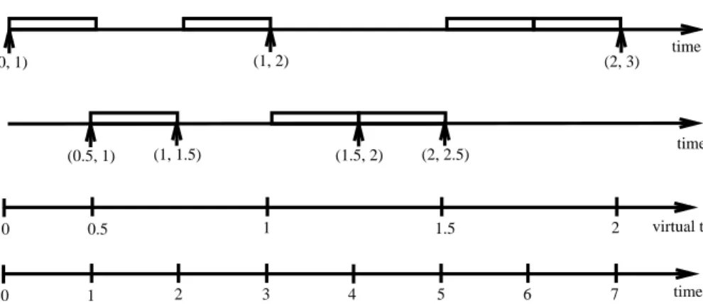
0 1 2 3 4 5 6 7 (0, 1) 0 0.5 1 (0.5, 1) (1, 1.5) (1, 2) (1.5, 2) 1.5 (2, 2.5) 2 time virtual time (2, 3) client 1 client 2 time time
Figure 1: An example of EEVDF scheduling involving two clients with equal weights w1= w2= 2. All
the requests generated by client1have length2, and all of the requests generated by client2are of length
1. Client1becomes active at time0(virtual time0), while client2becomes active at time1(virtual time
0:5). The arrows represent the times when the requests are initiated (the pair associated to each arrow represents the virtual eligible time and the virtual deadline of the corresponding request).
ve(1) = V (ti 0); (9) vd(k) = ve(k)+ r (k) wi ; (10) ve(k+1) = vd(k): (11)
Next, let us consider the more general case in which the client does not use the entire service time it has requested. Since a client never receives more service time than requested, we need to consider only the case when the client uses the resource for less time than requested. Let u(k)denote the service
time that client i actually receives during kth request. Then the only change in Eq. (9){(11), will be in
computing the eligible time of a new request. Specically, Eq. (11) is replaced by ve(k+1)= ve(k)+ u
(k)
wi : (12)
To clarify the ideas, let us take a simple example (see Figure 1). Consider two clients with weights w1 = w2 = 2 that issue requests with lengths r1 = 2, and r2 = 1, respectively. We assume that the
time quantum is of unit size (q = 1) and that client 1 is the rst one which enters competition at time t0 = 0. Thus, according to Eq. (9) and (10) the virtual eligible time for the rst request of client 1
is ve = 0, while its virtual deadline is vd = 1. Being the single client that has an outstanding eligible request, client 1 receives the rst quantum. At time t = 1, client 2 enters the competition. Since the virtual time increases at a constant rate during the interval [0;1) (i.e., 1
w1 = 0:5), its value at time t = 1
is V (1) = R 1 0
1
w1d = 0:5. After the second client enters the competition the slope of the virtual time
function becomes 1
w1 +w
2 = 0:25. Next, let us assume that client 2 makes its rst request before the
second quantum is allocated. Then at t = 1 there are two pending requests: one from client 1 with the virtual deadline 1 (which waits for another time quantum to fulll its request), and one from client 2 which has the same virtual deadline i.e., 1. In this situation we arbitrarily break the tie in the favor of client 2, which therefore receives the second quantum upon termination. Since this quantum fullls the current request of client 2, client 2 issues a new one with the virtual eligible time 1 and the virtual
deadline 1:5. Thus, at time t = 2 the single eligible request is the one of client 1, which therefore receives the next quantum. Further, at t = 3 there are again two eligible requests: the one of client 2 that has just become eligible, and the new request issued by client 1. Since the deadline of the second client's request (1.5) is earlier than the one of the rst client (2), the fourth quantum is allocated to the client 2. Further, Figure 1 shows how the next three quanta are allocated.
4 Fairness in Dynamic Systems
In this section we address the issue offairnessin dynamic systems. Throughout this paper, we assume that a dynamic system provides support for the following three operations: client joining the competi-tion, client leaving the competicompeti-tion, and changing the client's weight. In an idealized uid-ow system, supporting dynamic operations is trivial since at any moment of time the lag of any active client is zero. Unfortunately, in a system in which the service time is allocated in discrete time quanta, this is no longer true. In the remaining of this section we discuss how this aects the fairness in a dynamic system6. We
consider the following two questions:
1. What is the impact of a client with non-zero lag leaving, joining, or changing its weight on the other clients ?
2. When a client with non-zero lag leaves the competition, what should be its lag when it rejoins the competition ?
In answering the rst question, we start with a simple example. Let us assume that a client leaves the competition with a negative lag, i.e., after it has received more service time than it was entitled to. As we will show in Section 6, during any time interval, the total service time allocated to all active clients is equal to the service time that the clients should receive. Therefore, if a client leaves the competition with a negative lag, the remaining clients should have received less service time than they were entitled to. In short, a gain for one client translates into a loss for the other active clients. In this case, the question we need to answer is the following: How should the loss be distributed among the remaining active clients in order to attain fairness ? We answer this question by assuming that whenever a dynamic operation takes place, the eect (i.e., the resulting gain or loss) is proportionallydistributed among all active clients. In other words, each active client will inherit a gain/loss proportional to its weight. Besides its intuitive appeal, as we will show, this policy has another advantage: it can be easily implemented by simply updating the virtual time. We note that although this policy is similar to the one employed by Waldspurger and Weihl in their stride scheduling algorithm [29, 30], the two policies are not equivalent. The dierence consists in the way in which the virtual time is updated when a client leaves or joins the competition: while in stride scheduling only the slope of the virtual time 7is updated, in our algorithm
the value of the virtual time is updated as well (see Eq. 18, 19, 20 in this section).
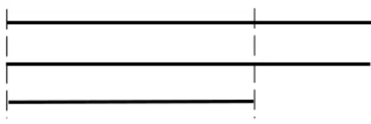
To better understand our reasons in considering the above policy, let us consider the followingexample. Suppose that three clients with zero lags become active at time t0, and at time t client 3 leaves the
competition (see Figure 2). Further, we discuss the impact of client 3 leaving the competition on the other two clients.
6These issues were also addressed by Waldspurger and Weihl in the context of their stride scheduling algorithm [30]. 7Instead virtual time, stride scheduling uses an equivalent concept, called
t0 t client 1
client 2 client 3
Figure 2: The three clients become active at timet0. At timet, client3leaves the competition.
Since the number of active clients and their shares do not change during the interval [t0;t), the slope
of the virtual time during this interval is constant and equal to 1
w1+w2+w
3. Then from Eq. (3) and (6),
the lag of each client at time t is
lagi(t) = wi t?t 0
w1+ w2+ w3 ?si(t
0;t); i = 1;2;3: (13)
Next, we turn our attention to the clients 1 and 2 which remain active after client 3 leaves the competition. Since EEVDF is a work-conserving8algorithm, the total service time received by all active clients during
the interval [t0;t) is equal to t ?t
0. From here, the service time allocated to the rst two clients during
this interval can be expressed as t?t 0
?s
3(t0;t). Let t
+ be the time immediatelyafterclient 3 leaves
the competition, where by neglecting the leaving operation overhead, we have t+ !t.
Now, what is the service time that clients 1 and 2 should have received at time t+ ? A natural
and intuitive approach would be to simply divide the entire service time received by both clients (i.e., t?t
0 ?s
3(t0;t)) proportional to the clients' weights, i.e.,
Si(t0;t + ) = (t?t 0 ?s 3(t0;t)) w i w1+ w2 ; i = 1;2; (14) We note that if lag3(t)
6
= 0, then this result is dierent from the service time each client should have received just before the departure of client 3, i.e., (t?t
0) wi w1 +w 2 +w
3 (i = 1;2;3). This is because once
client 3 leaves, the remaining two clients will proportionally support the eventual loss or gain in the service time. Next, we show that in the EEVDF algorithm this is equivalent to a simple translation of the virtual time. By replacing s3(t0;t) from Eq. (13) into Eq. (14), we obtain
Si(t0;t +) = (t ?t 0) wi w1+ w2+ w3 + wi lag3(t) w1+ w2 (15) = wi(V (t)?V (t 0)) + wi lag3(t) w1+ w2 ; i = 1;2: Finally, from Eq. (6) and (15) it follows that
V (t+) = V (t) + lag 3(t)
w1+ w2
; i = 1;2: (16)
Thus, to maintain the fairness among the remaining clients, the virtual time should be updated according to the lag of the client which leaves the competition (as shown by the above equation). Since t+ is
asymptotically close to t, the service time received by any client at time t+ is equal to the service time
it has received at time t (i.e., si(t0;t) = si(t0;t
+)). From here, the lags of the rst two clients at t+ can
be computed as lagi(t+) = w i(V (t+) ?V (t 0)) ?si(t 0;t +) = lag i(t) + wi lag3(t) w1+ w2 ; i = 1;2: (17)
8A scheduling algorithm is said to be
work-conserving if the resource cannot be idle while there is at least one active client (see Section 6 for details).
Therefore when client 3 leaves, its lag is proportionallydistributed among the remaining clients, which is in accordance with our interpretation of fairness. By generalizing Eq. (16), we derive the following updating rule for the virtual time when a client j leaves the competition at time t
V (t) = V (t) + lagP j(t)
i2A(t +
)wi
: (18)
Correspondingly, when a client j joins the competition at time t, the virtual time is updated as follows V (t) = V (t)? lagj(t) P i2A(t + )wi ; (19) where A(t
+) contains all the active clients immediately after client j joins the competition, and lag
j(t)
represents the lag with which client j joins the competition. Although it might not be clear at this point, by updating the virtual time according to Eq. (18) and (19) we ensure that the sum over the lags of all active clients is always zero. This can be viewed as a conservation property of the service time, i.e., any time a client receives moreservice time than its share, there is at least another client that receives less. We note that if the lag of the client that leaves or joins the competition is zero, then according to Eq. (18) and (19) the virtual time does not change.9
We note that changing the weight of an active client is equivalent to a leave and a rejoin operation that take place at the same time. To be specic, suppose that at time t the weight of client j is changed from wj to w0
j. Then this is equivalent to the following two operations: client j leaves the competition at
time t, and rejoins it immediately (at the same time t) having weight w0
j. By adding Eq. (18) and (19),
we obtain V (t) = V (t) +(P lagj(t) i2A(t)wi) ?wj ? lagj(t) (P i2A(t)wi) ?wj+ w 0 j: (20)
As for join and leave operations, notice that the virtual time does not change when the weight of a client withzerolag is modied. Thus, in a system in which any client is allowed to join, leave, or change its weight only when its lag is zero, the variation of the virtual time is continuous.
Now let us turn our attention to the second question. We need to decide whether a client that becomes passive without using its entire share could use it when it again becomes active next time, and whether a client that leaves the competition after it has used more service time than its share should be penalized when it rejoins the competition. To be specic, consider a client that leaves the competition with a positive lag (i.e., after it has received less service time than it was entitled to). Then the question is whether the client should receive any compensation when it rejoins the competition. Unfortunately, there is no simple answer to this question. If we decide not to compensate, then the lost service time may accumulate over multiple periods of activity, and consequently, over large intervals of time the client may receive signicantly less service time than it is entitled to. On the other hand, if we decide to compensate a client for the lost service when it rejoins the competition, this might hamper other clients. To see why, consider the following example. Suppose that before time t there are two active clients 1 and 2, and at time t client 2 becomes passive with a positive lag, lag2(t) > 0. Next, assume that at a subsequent time
t0client 2 rejoins the competition, while another client 3 is active (we assume that at this time client 1
is no longer active). Then client 2 will have to recover the service time that it has lost to client 1, at the expense of client 3 ! Consequently, client 3 will indirectly lose some service time because client 2 has not used its entire service time while it was previously active, which is not fair.
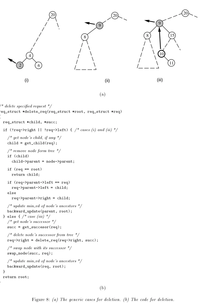
5 Algorithm Implementation
Since, as we have seen in the previous section, there is no clear answer on what isfairto do with the lag of a client when it rejoins the competition, in this section we present three strategies for implementing the EEVDF algorithm. The characteristics of these strategies are dictated by the decision on whether a client could leave, join, or change its weight when its lag is non-zero, and by the decision on whether a client receives compensation or it is penalized when it rejoins the competition.
Strategy 1.
In this strategy a client may leave or join the competition at any time, and depending on its lag it is either penalized or it receives compensation when it rejoins the competition. More precisely, if the client leaves the competition at time t, and rejoins at t0, then lag(t) = lag(t0). Each time an eventoccurs (e.g., a client joining, leaving, or changing the weight of a client), the virtual time is updated according to Eq. (18), (19), and (20) respectively. Finally, we note that this strategy is appropriate for systems where it is desirable to maintain fairness over multiple periods of client activity. In Appendix A we give an example of how this strategy might be actually implemented.
Strategy 2.
This strategy is similar to the previous one with the only dierence being that the lag is not preserved after a client leaves the competition, i.e., any client that (re)joins the competition has zero lag. This strategy is appropriate for those systems in which the events that cause the clients to become active are independent. This is similar to a real-time system in which the processing time required by an event is assumed to be independent of the processing time required by any other event.Strategy 3.
In this strategy a client is allowed to leave, join, or change its weight, only when its lag is zero. Thus, in this case, there is no need to update the virtual time when a dynamic operation takes place. On the other hand, some complexity is added in ensuring that when these events occur the lag is indeed zero. In order to ensure that all events involve only clients with zero lag, we need to update the slope of the virtual time at the corresponding times in the uid-ow system. The main problem in implementing this strategy is to update the slope of the virtual time when a client leaves the competition with a positive lag.10 In this case the time at which the client should leave the competition in theuid-ow system is smallerthan the corresponding time in the real system. A solution would be to \undo" all the modications in the system that occurred between the time when the client should leave the competition in the uid-ow system and the time when it actually leaves. Unfortunately, this solution is very expensive to implement; it requires to store the event history and, in addition, the \undo" operation may involve a high overhead. In solving this problem, we assume that no event occurs during any time quantum. We note that this assumption is not as restrictive as it appears. For example, in the processor case, this is a realistic assumption since, in general, the scheduling algorithm executes only between time quanta. On the other hand, in communication networks we do not need to enforce this assumption since the service time (i.e., transmission time) is assumed to be known, before the request is initiated. The basic mechanisms to implement this strategy, under the assumption that no event can occur during a time quantum is given below.
First, assume that a client wants to leave the competition when its lag is negative. In this case, the idea is simply todelay the client until its lag becomes zero. This is done by issuing a dummy request of
10We note that in a system in which the client always uses the entire service time it has requested, by using Eq. ( 9){(11) we can compute the virtual time when the client should leave in the uid-ow system as the virtual deadline of the client's last request. This is the approach used by Parekh and Gallager in their Packet-by-Packet Generalized Processor Share algorithm [23].
zero length. This approach is motivated by the fact that, in this case, the eligible time is always chosen such that the lag is zero. Since a request cannot be processed before it becomes eligible, and since the virtual eligible time of the dummy request is equal to its deadline (see Eq. (10)), it follows that this request will be processed after its deadline. Thus, by using a request of zero length, we have reduced the case of a client which leaves with a negative lag to the case of a client which leaves with a nonnegative lag and therefore we further consider only the later case. As we will show in Section 6, in a system in which the virtual time varies continuously (such as in our system), a request is guaranteed to be fullled no latter than a time quantum after its deadline. Thus, between the moment when the lag of the client becomes zero, and the moment when the request is fullled, no other time quanta are allocated. Since
noevent occurs during this time quantum, it will not make any dierence whether we update the virtual time after the time quantum expires, instead of exactly when the lag becomes zero.
A second question regarding this strategy is what to do with the remaining service time when the client leaves before its last request has been fullled. Here we take the simplest approach: the extra time quanta that are no longer used by the client are randomly allocated to other active clients without
chargingthem, i.e., their received service times and theirs lags are not updated. Although more complex allocation schemes might be devised, they are not necessary to achieve the goal of this strategy which is to guarantee that as long as a client competes for the resource it will receive atleastits share.
6 Fairness Analysis of the EEVDF Algorithm
In this section we determine bounds for the service time lag. First we show that during any time interval in which there is at least one active client, there is also at least one eligible pending request (Lemma 2). A direct consequence of this result is that the EEVDF algorithm is work-conserving, i.e., as long as there is at least one active client the resource cannot be idle. By using this result, in Theorem 1 we give tight bounds for the lag of any client in a steady system (see Denitions 1 and 2 below). Finally, we show that in the particular case when all the requests have durations no greater than a time quantum q, our algorithm achieves tight bounds which are optimal with respect to any proportional share allocation algorithm (Lemma 5).
Throughout this section we refer to any event that can change the state of the system, i.e., a client joining or leaving the competition, and changing the client's weight, simply asevent. We introduce now some denitions to help us in our analysis.
Denition 1
A system is said to besteady
if all the events occurring in that system involve only clients with zero lag.Thus, in a steady system the lag of any client that joins, leaves, or has its weight changed, is zero. Recall that in a system in which all events involve only clients having zero lags the virtual time is continuous. As we will see, this is the basic property we use to determine tight bounds for the client lag. The following denition restricts the notion of steadiness to an interval.
Denition 2
An interval is said to besteady
if all the events occurring in that interval involve only clients with zero lag.We note that a steady system could be alternatively dened as a system for which any time interval is steady. The next lemma gives the condition for a client request to be eligible.
Lemma 1
Consider an active clientk with a positive lag at timet, i.e.,lagk(t)0; (21)
Then clientk has a pending eligible request at timet.
Proof.
Let r be the length of the pending request of client k at time t (recall that an active client has always a pending request), and let ve and vd denote the virtual eligible time and the virtual deadline of the request. For the sake of contradiction, assume the request is not eligible at time t, i.e.,ve > V (t) (22)
Let t0 be the time when the request was initiated. Then from Eq. (7) we have
ve = V (tk
0) + s
k(tk0;t 0)
wk : (23)
Since between t0and t the request was not eligible, it follows that the client has not received any service
time in the interval [t0;t), and therefore s
k(tk0;t 0) = s k(tk0;t). By substituting sk(t k 0;t 0) to s k(tk0;t) in Eq.
(23) and by using Eq. (3) and (6) we obtain
lagk(t) = wk(V (t)?V (tk 0)) ?sk(tk 0;t) (24) = wk(V (t)?V (tk 0)) ?wk(ve?V (tk 0)) = wk(V (t)?ve):
Finally, from Ineq. (22) it follows that lagk(t) < 0, which contradicts the hypothesis and therefore proves
the lemma.
From Lemma 1 and from the fact that any zero sum has at least a nonnegative term, we have the following corollary.
Corollary 1
Let A(t) be the set of all active clients at timet, such thatX
i2A(t)
lagi(t) = 0: (25)
Then there is at least one eligible request at timet.
The next lemma shows that at any time t the sum of the lags over all active clients is zero. An immediate consequence of this result and the above corollary is that at any time t at which there is at least one active client, there is also at least one pending eligible request in the system. Thus, in the sense of the denition given in [23], the EEVDF algorithm iswork-conserving, i.e., as long as there are active clients the resource is busy.
Lemma 2
At any moment of timet, the sum of the lags of all active clients is zero, i.e,X
i2A(t)
Proof.
The proof goes by induction. First, we assume that at time t = 0 there is no active client and therefore Eq. (26) is trivially true. Next, for the induction step, we show that Eq. (26) remains true after each one of the following events occurs: (i) a client joins the competition, (ii) a client leaves the competition, (iii) a client changes its weight. Finally, we show that (iv) during any interval [t;t0) in whichnone of the above events occurs if Eq. (26) holds at time t, then it also holds at time t0.
Case (i). Assume that client j joins the competition at time t with lag lagj(t). Let t? denote the time
immediately before, and let t+ denote the time immediately after client j joins the competition, where
t+and t?are asymptotically close to t. Next, let W(t) denote the total sum over the weights of all active
clients at time t, i.e., W(t) = P
i2A(t)wi(t), and by convenience let us take lagj(t
?) = lag j(t). Since t? !t +we have s i(ti0;t ?) = s i(ti0;t
+). Then from Eq. (3) we obtain:
lagi(t+) = lag i(t?) + S i(ti0;t +) ?Si(ti 0;t ?)
Further, by using Eq. (6) and (19), the lag of any active client i at time t+ (including client j) is
lagi(t+) = lag i(t?) ?lagj(t) w i W(t+): (27) Since A(t +) = A(t ?)
[fjg, and since from the induction hypothesis we have P
i2A(t ?
)lagi(t
?) = 0, by
using Eq. (27), we obtain
X i2A(t + ) lagi(t+) = X i2A(t + ) (lagi(t?) ?lagj(t) w i W(t+)) (28) = X i2A(t + ) lagi(t?) ?lagj(t) P i2A(t + )wi W(t+) = X i2A(t ? ) lagi(t?) + lag j(t?) ?lagj(t) = 0:
Case (ii). The proof of this case is very similar to the one of the previous case; therefore we omit it here. Case (iii). Changing the weight of a client j from wj to w0
j at time t can be viewed as a sequence of two
events: rst, client j leaves the competition at time t; second, it joins the competition at the same time t, but with weight w0
j. Thus, the proof of this case reduces to the previous two cases.
Case (iv). Consider an interval [t;t0) in which no event occurs, i.e., no client leaves or joins the competition
and no weight is changed during the interval [t;t0). Next, assume that P
i2A(t)lagi(t) = 0. Then we shall
prove thatP
i2A(t 0
)lagi(t
0) = 0. By using Eq. (3) and (6) we obtain X i2A(t 0 ) lagi(t0) = X i2A(t 0 ) (Si(ti0;t 0) ?si(ti 0;t 0)) (29) = X i2A(t) (Si(ti0;t) ?si(ti 0;t)) + X i2A(t) (Si(t;t0) ?si(t;t 0)) = X i2A(t) lagi(t) + X i2A(t) Si(t;t0 )? X i2A(t) si(t;t0 ) = X i2A(t) wi(V (t0) ?V (t))? X i2A(t) si(t;t0) = (t0 ?t)? X i2A(t) si(t;t0):
Next we show that the resource is busy during the entire interval [t;t0). For contradiction assume this is
not true. Let l denote the earliest time in the interval [t;t0) when the resource is idle. Similarly to Eq.
X i2A(l) lagi(l) = (l?t)? X i2A(t) si(t;l):
Since the resource is not idle at any time between t and l, it follows that the total service time allocated to all active clients during the interval [t;t0) (i.e.,
P
i2A(t)si(t;l)) is equal to l
?t. Further, from the
above equation we have P
i2A(l)lagi(l) = 0. But then from Lemma 1 it follows that there is at least one
eligible request at time l, and therefore the resource cannot be idle at time l, which proves our claim. Further, with a similar argument, it is easy to show thatP
i2A(t 0
)lagi(t
0) = 0 which completes the proof
of this case.
Since these are the only cases in which the lags of the active clients may change, the proof of the lemma follows.
The following lemma gives the upper bound for the maximum delay of fullling a request in a steady system. We note that this result is similar to the one obtained by Parekh and Gallager [23] for their Generalized Processor Sharing algorithm, i.e., in a communication network, a packet is guaranteed not to miss its deadline by more than the time required to send a packet of maximum length.
Lemma 3
In a steady system any request of any active client k is fullled no later thand + q, wheredis the request's deadline, and q is the size of a time quantum.
Proof
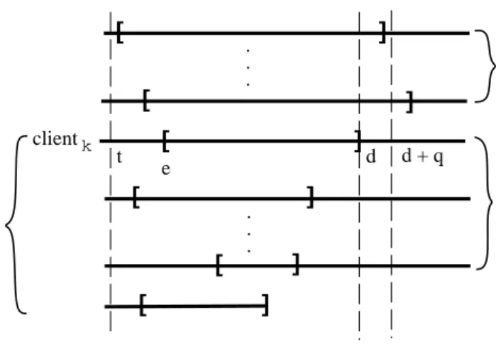
. Let e be the eligible time associated to the request (with deadline d) of client k. Consider the partition of all the active clients at time d, into two sets B and C, where set B contains all the clients that have at least a deadline in the interval [e;d] , and set C contains all the other active clients (see Figure 3). Let t be the latest time no greater than d at which a client in C receives a time quantum, if any. Further we consider two cases whether such a t exists or not.Case 1
(t exists). Here we consider two sub-cases whether t2[e;d), or t < e. First assume that a clientin C receives a time quantum at a time t2[e;d). Since all the deadlines of the pending requests issued
by clients in C are larger than d, this means that at time t the pending request of client k is already fullled. Consequently, in the rst sub-case the request of client k is fullled before time d.
For the second sub-case, let us D denote all the active clients that have at least one eligible request with the deadline in the interval [t;d) (see Figure 3). Further, let D() denote the subset of D containing the active clients at time . Since a time quantum is allocated to a client in C at time t, it follows that no other client with an earlier deadline is eligible at t. For any client j belonging to D(t), let ej be the
eligible time of its pending request at time t. Since the deadlines of these requests are no greater than d (and therefore smaller than any deadline of any client in C), it follows that all these pending requests are not eligible at time t, i.e., t < ej. Notice that besides the clients in D(t), the other clients that belong
to D are those that eventually join the competition after time t. For any client j in D that joins the competition after time t, we take ej to be the eligible time of its rst request.
Next, for any client j belonging to D, let dj denote the largest deadline no greater than d of any of
its requests (notice that the eligible time ej and the deadline dj might not be associated to the same
request). From Eq. (10) it easy to see that after client j receives Sj(ej;dj) time units, all its requests
in the interval [ej;dj) are fullled. Thus, the service time needed to fulll all the requests which have
. . . . . . ] ] ] ] ] client [ [ k t e B C d D(t) d + q [ [ [ ] [
Figure 3: The current pending request of client khas the eligible timee and deadline d. Set B contains all the active clients that have at least one request with the deadline in the interval [e;d], while set C
contains all the other active clients. Timetrepresents the largest time no greater thandat which a client from C receives a time quantum. Finally, setD(t) contains all the active clients at timet that have at least one eligible request with the deadline in the interval[t;d).
X j2D Sj(ej;dj) =X j2D (Z d j ej wj P i2A()wi d): (30)
By decomposing the above sum over a set of disjoint intervals Jl = [al;bl) (1 l m) covering [t;d),
such that no interval contains any eligible time or deadline of any client belonging to D, we can rewrite Eq. (30) as X j2D Sj(ej;dj) =Xm l=1 (Z b l al P i2D(al)wi P i2A(al)wi d) <Xm l=1 (Z b l al d) = m X l=1 (bl?al) = d?t; (31)
The above inequality results from the fact that D() is a proper subset ofA() at least for some
sub-intervals Ji (otherwise, ifA() is identical to D() over the entire interval [t;d), sets C and C
0would be
empty).
Assume that at time d+ q the request of client k (having the deadline d) is not fullled yet. Since no client in C can be served before the request of client k is fullled, it follows that the service time between t+q and d+q is allocated only to the clients in D. Consequently, during the entire interval [t+q;d+q), there are d?t service time units to be allocated to all clients in D. Next, recall that any client j belonging
to D will not receive any other time quantum after its request having deadline djis eventually fullled, as
long as the request of client k is not fullled. This is simply because the next request of client j will have a deadline greater than d. But according to Eq. (31) the service time required to fulllallthe requests having the deadlines in the interval [t;d) is less than d?t, which means that at some point the resource
is idle during the interval [t + q;d + q). But this contradicts the fact that EEVDF is work-conserving, and therefore proves this case.
Case 2.
(t does not exist) In this case we take t to be the time when the rst client joins the competition. From here the proof is similar to the one for the rst case, with the following dierence. Since set C is empty, all the time quanta between t and d are allocated to the clients in D, and therefore, in this case, we show that in fact client k does not miss the deadline d.Following we give a similar result for a steady interval. Mainly, we show that for certain subintervals of a steady interval the same bound holds. This shows that a system which allows clients with non-zero lag to join, leave, or to change their weight, will eventually reach a steady state.
Lemma 4
LetI = [t1;t2)be a steady interval, and letdm be the largest deadline among all the pendingrequests of the clients with negative lags which are active at t1. Then any request of any active client k
is fullled no later than d + q, if d2[dm;t 2).
Proof.
Similarly to the proof of Lemma 3, we consider the partition of all the active clients at time d, into two set B and C, where set B contains all the active clients that have at least a deadline in the interval [e;d] , and set C contains all the other clients. Similarly, we let t denote the latest time in the interval [t1;d) when a client in C receives a time quantum, if any. Further, we consider two cases whethersuch t exists or not.
Case 1.
(t exists) The proof proceeds similarly to the one for Case 1 in Lemma 3.Case 2.
(t does not exist) In this case we consider two sub-sets of C: C? containing all clients in Cthat had negative lags at time t1, and C
+ containing all the other clients in C. Since no client belonging
to C? receives any time quantum before d
m it follows that no pending request of any client in C? is
fullled before its deadline (recall that the deadlines of all the other clients with negative lags at t1 are dm) and therefore all clients in C
? will have nonnegative lags at time d
m. On the other hand, since
all clients in C+ had nonnegative lags at time t
1, and since they do not receive any time quanta between
t1and dm, all of them will have positive lags at dm. Thus, we have X
i2C
lagi(d) > 0 (32)
On the other hand, we note that if the request of client k is not fullled before its deadline, then no other client belonging to B will receive any other time quantum after its last request with the deadline no greater than d is fullled. But then from Eq. (3) it follows that their lags as well as the lag of client k are positive at time d, i.e.,
X
i2B
lagi(d)0 (33)
Further, by adding Eq. (32) and (33), we obtain
X
i2A(d)
lagi(d) > 0 (34)
which contradicts Lemma 2, and therefore completes the proof.
The next theorem gives tight bounds for a client's lag in a steady system.
Theorem 1
The lag of any active client kin a steady system is bounded as follows,?rmax< lagk(d) <max(rmax;q); (35)
where rmax represents the maximum duration of any request issued by clientk. Moreover, these bounds
Proof
. Let e and d be the eligible time and the deadline of a request with duration r issued by client k. Since Sk increases monotonically with a slope no greater than one (see Eq. (4)), from Eq. (3) it followsthat the lag of client k decreases as long as it receives service time, and increases otherwise. Further, since a request is not serviced before it is eligible, it is easy to see that the minimum lag is achieved when the client receives the entirely service time as soon as the request becomes eligible. In other words, the minimum lag occurs at time e + r, if the request is fullled by that time. Further, by using Eq (3) we have lagk(e + r) = Sk(tk0;e + r) ?sk(tk 0;e + r) (36) = Sk(tk0;e) + Sk(e;e + r) ?(sk(tk 0;e) + sk(e;e + r))
= lagk(e) + Sk(e;e + r)?sk(e;e + r)
From the denition of the eligible time (see Section 2) we have lagk(e) 0, and thus from the above
equation we obtain
lagk(e + r)Sk(e;e + r)?sk(e;e + r) >?sk(e;e + r)?r: (37)
Since this is the lower bound for the client's lag during a request with duration r, and since rmaxrepresents
the maximum duration of any request issued by client k, it follows that at a any time t while client k is active we have
lagk(t)?rmax: (38)
Similarly, the maximum lag in the interval [e;d) is obtained when the entire service time is allocated as late as possible. Since according to Lemma 3, the request is fullled no later than d + q, it follows that the latest time when client k should receive the rst quantum is d + q?r. We consider two cases:
rq and r < q. In the rst case d + q?rd, and therefore we obtain Sk(e;d + q?r) < Sk(e;d) = r.
Let t1 be the time at which the request is issued. Further, from the denition of the eligible time, and
from the fact that the client is assumed that it does not receive any time quantum during the interval [t1;d + q
?r), we have for any time t while the request is pending
lagk(t) Sk(tk 0;d + q ?r)?sk(tk 0;d + q ?r) (39) = Sk(tk0;e) + Sk(e;d + q ?r)?sk(tk 0;t 1) ?sk(t 1;d + q ?r) = (Sk(tk0;e) ?sk(tk 0;t 1)) + Sk(e;d + q ?r)?sk(t 1;d + q ?r) = Sk(e;d + q?r) < r:
Since the slope of Sk is always no greater than one, in the second case we have Sk(e;d + q ?r) =
Sk(e;d) + Sk(d;d + q?r) < r + q?r = q, and from here we obtain
lagk(t)Sk(e;d + q?r) < q: (40)
Finally, by combining Eq. (39) and (40) we obtain lagk(t) < max(q;r). Thus, at any time t while the
client is active we have
To show that the bound lagk(t) >?rmaxis asymptotically tight, consider the following example. Let
w1, w2be the weights of two active clients, such that w1
w
2. Next, suppose that both clients become
active at time t0 and their rst requests have the lengths rmax and r 0
max, respectively. We assume that
rmax and r0
max are chosen such that the virtual deadline of the rst client's request is smaller than the
virtual deadline of the second client's request, i.e., t0+
rmaxw
1 < t 0 +
r0
maxw
2 . Then client 1 receives the
entire service time before client 2, and thus from Eq. (3) we have lag1(rmax) = S1(t0;t0+ rmax)
?rmax.
Next, by using Eq. (4) we obtain S1(t0;t0+ rmax) =
w1
w1 +w
2, which approaches zero when
w1
w2
!1, and
consequently lag1(rmax) approaches
?rmax.
To show that the bound lagk(t) < max(rmax;q) is asymptotically tight, we use the same example.
However, in this case we assume that the virtual deadline of the rst request of client 1 is earlier than the virtual deadline of the rst request of client 2, such that client 1 receives its entire service time just prior to its deadline. Since the details of the proof are similar with the previous case we do not show them here.
Notice that the bounds given by Theorem 1 apply independently to each client and depend only on the length of their requests. While shorter requests oer a better allocation accuracy, the longer ones reduce the system overhead since for the same total service time fewer requests need to be generated. It is therefore possible to trade between the accuracy and the system overhead, depending on the client requirements. For example, for an intensive computation task it would be acceptable to take the length of the request to be in the order of seconds. On the other hand, in the case of a multimedia application we need to take the length of a request no greater than several tens of milliseconds, due to the delay constraints. Theorem 1 shows that EEVDF can accommodate clients with dierent requirements, while guaranteeing tight bounds for the lag of each client during a steady interval. The following corollary follows directly from Theorem 1.
Corollary 2
Consider a steady system and a client k such that no request of clientk is larger than a time quantum. Then at any timet, the lag of clientk is bounded as follows:?q < lagk(t) < q: (42)
Next we give a simple lemma which shows that the bounds given in Corollary 3 are optimal, i.e., they hold for any proportional share algorithm.
Lemma 5
Given any steady system with time quanta of sizeqand any proportional share algorithm, the lag of any client is bounded by?q and q.Proof.
Consider n clients with equal weights that become active at time 0. We consider two cases: (i) each client receives exactly one time quantum out of the rst n quanta, and (ii) there is a client k which receives more than a time quanta. From Eq. (3), it is easy to see that, at time q, the lag of the client that receives the rst quantum islag(q) = qn?q: (43)
Similarly, the lag of the client which receives the nthtime quantum is (at time n?1, immediately before
it receives the time quantum)
lag(q(n?1)) = q?
q
For contradiction, assume that there is a proportional share algorithm that achieves an upper bound smaller than q, i.e., q?, where is a positive real. Then by taking n > q, from Eq. (44), it follows that
lag(q(n?1)) > q? which is not possible. Similarly, it can be shown that no algorithm can achieve a
lower bound better than -q.
For the second case (ii), notice that since client j receives more than one time quanta, there must be another client k that does not receive any time quanta in the rst n time units. Then it is easy to see that the lag of client j is smaller than?q after it receives the second time quantum, and the lag of client
k is larger than q after just before receiving its rst time quantum, which completes our proof.
7 Related Work
In this section we present a compressive overview of the related work. We classify the scheduling algo-rithms as follows: time-dependent priority, real-time, fair queueing, and proportional share.
7.1 Time-Dependent Priority
Many of the existing operating systems rely on the concept of priorityto allocate processing time to competing processes [25]. In the static priority schemes, a process with higher priority has absolute precedence over a process with lower priority. Unfortunately, this schemes are inexible and may lead to starvation [25]. In trying to overcome these problems, several solutions were proposed. One of the best-known schemes is decay usage scheduling [13] which tries to ensure fairness by changing the process priorities according to their recent CPU usage. This policy was implemented in many operating systems, such as Unix BSD [16] and System V [1]. The main drawback of this policy is that it oers only a crude control over resource allocation during short periods of time.
Recently, Fong and Squillante have proposed a new scheduling discipline called Time-FunctionSchedul-ing (TFS) [11]. The priority of a client in TFS is dened by a time-dependent function, i.e., the priority increases linearly with time while the client waits to be scheduled, and it is reinitialized to a predened value whenever the client is scheduled. In TFS clients are partitioned in disjoint classes based on their characteristics and scheduling objectives. All clients belonging to the same class have associated the same time-dependent function and are organized in a FCFS queue. By serving them in a round-robin fashion, the scheduler ensures that the client with the highest priority in that class is always at the front of the queue. Thus to select the client with the highest overall priority it is enough to search among the clients which are at the front of their queues. In this way, the dispatch operation can be eciently implemented in O(logc), where c represents the total number of classes. On the other hand, the time-complexity of updating clients' priorities is O(clogc). TFS provides eective and exible control over resource alloca-tion and it can be used to achieve general scheduling objectives such as relative per-class throughputs and low waiting time variance. Although somewhat indirectly, TFS can also archive proportional share allocation by assigning an equal share to each client in the same class. However, the algorithm accuracy depends on the frequency at which the clients' priorities are updated. Since the updating operation is rather expensive this limits the allocation accuracy that can be achieved.
7.2 Real-Time
Real-time systems were specically developed for critical time tasks which require strong deadline guar-antees. These tasks are characterized by a sequence of events that arrive in a certain pattern (usually
periodic). Each event is described by its predicted service time and a deadline before which the event should be processed.
Two of the most popular algorithms for scheduling periodic tasks,rate monotonic(RM) andearliest deadline rst(EDF), were proposed and analyzed by Liu and Layland in [18]. In RM, tasks are assigned priorities in the decreasing order of their periods, i.e., the task with the smallest period has the highest priority. While in RM the priorities are xed, in EDF they change dynamically whenever a task initiates a new request. More precisely, the EDF algorithm assigns priorities to tasks corresponding to the deadlines of their current requests, i.e., the task which has the request with the earliest deadline is assigned the highest priority.
We note here that in a static uid-ow system (in which the weights and the number of active clients do not change) the EEVDF and EDF algorithms are equivalent. To see why, consider how EEVDF behaves when a new request with an earlier deadline than the process that is currently executing is issued. In this case, as soon as the current time quantum expires, the new request is scheduled for execution. Since in an idealized uid-ow model the size of a time quantum is arbitrarily small, this is equivalent to schedule the new request as soon as it arrives, which is identical to the policy employed by EDF.
In order to guarantee that all tasks will meet their deadlines, both RM and EDF impose strict admission policies. Specically, Liu and Layland [18] have shown that under the EDF policy all tasks will meet their deadlines as long as the processor is not over-utilized (i.e., its utilization is 100%).
Similarly, for the RM algorithm, they have given a schedulability test with the worst case processor utilization of 69%. For a specied set of tasks, this bound can be improved by using the exact analysis given by Lehoczky, Sha, and Ding in [17]. Unfortunately, this analysis is more expensive, which makes it less appealing for practical implementations. Besides ensuring a higher processor utilization, another advantage of EDF versus RM is that, for the same set of tasks, it never generates more preemptions than RM, which reduces the context-switching overhead. On the other hand, since it uses xed priorities RM is simpler and slightly more ecient to implement than EDF. Finally, another advantage of RM is that in case of overload the tasks with higher priorities will still meet their deadlines at the expense of tasks with lower priorities, while under the EDF algorithm all tasks could miss their deadlines.
Both RM and EDF were the solutions of choice used to add support for continuous media and real-time applications to the existing operating systems. For example, in designing an application platform for distributed multimedia applications, Coulsonet al[8] use the EDF algorithm for processor scheduling. Mercer, Savage, and Tokuda consider both RM and EDF algorithms in developing a exible higher level abstraction, calledprocessor capacity reserves[20, 21], specically designed for measuring and controlling processor usage in a microkernel system. In their model, each client (thread) has associated a reserve to which its computation time is charged. The scheduler uses the usage measurements for each client to control and enforce its reservation.
Unlike the above approaches which try to add support for real-time applications such as multimediaby extending and/or modifyingthe general purpose CPU schedulers in the existing operating systems, Bollela and Jeay [4] take a more radical approach. Their idea is to partition the processor and other shared system resources into two virtual machines: one machine running a general purpose operating system, and the other one running a real-time kernel support. Specically, the CPU is multiplexed between the two systems, each operating system running alternatively for a predened time slice. While this approach achieves a high level of isolation between general purpose and real-time applications, running two dierent operating systems increases both the overhead and the resource requirements in the system.
In general, real-time based schedulers do not provide an integrated solution for continuous media, interactive, and batch applications. For this reason, general purpose operating systems that use real-time based schedulers for supporting continuous media and interactive applications, also employ more conven-tional schedulers (such as round-robin) for batch activities. Compared to proporconven-tional-share schedulers, real-time schedulers are more restrictive and less exible. As an example, when an application terminates it is dicult to eciently redistribute its share among the applications that are still active. Finally we note that although real-time based schedulers provide stronger timeliness guarantees, the guarantees of-fered by the EEVDF algorithm (i.e., a deadline is never missed by more than a time quantum) are good enough to accommodate a broad range of real-time applications.
Recently, Jeay and Bennette have proposed a new abstraction for multimedia applications, called
rate-based execution (RBE) [13]. In RBE a process is characterized by three parameters: x, y, and d, where x represents the number of events that arrive during a time interval with the duration y, and d represents the desired maximumelapsed time between the delivery of an event and the completion of that event. Like EEVDF, RBE does not make any assumptions about the interarrival times, and about the distribution of the processing time during y time units. We note that specifying parameters x and y is equivalent to specifying the share that the process should receive during a time interval with the duration y. While RBE provides better control over the maximum elapsed time d (in the EEVDF this is implicitly determined from the client share and the request duration), the EEVDF provides more exibility in share allocation over time intervals of arbitrary length. Moreover, although RBE generalizes the traditional real-time models, it does not address the problem of supporting batch and multimedia applications in an integrated environment.
Nieh and Lam have developed a novel integrated processor scheduler that provides support for mul-timedia applications in a general purpose operating system [22]. Similarly to a request in EEVDF, they associate to each client aminimum execution ratewhich is dened as the desired fraction of the processing time that the client should receive in a given interval. For continuous media and interactive applications the minimum execution rates result directly from their time constraints, while for batch applications the minimum execution rates express their minimum acceptable rates of forward progress. These rates are translated into a series of deadlines, which are similar to the deadlines of the clients' requests in EEVDF. The scheduler attempts to meet these deadlines by using an EDF algorithm. In addition, the scheduler assigns to each activity a priority. When the system is overloaded, the scheduler tries to meet the time constraints for the clients with higher priorities at the expense of the clients with lower priorities.
We note t