Value at Risk: A Comparative Analysis

(1)

THE ACADEMY OF ECONOMIC STUDIES, BUCHAREST

DOFIN MASTER PROGRAM

Value at Risk: A Comparative

Analysis

- Dissertation Paper -

Tutor,

Prof. Dr. Moisă ALTĂR

Student,

(2)

Bucharest 2008

Abstract

This study develops a comparative analysis concerning Value at Risk measure for a portfolio consisting of three stocks traded at Bucharest Stock Exchange. The analysis set out from 1-day, 1% VaR and has been extended in two directions: the volatility models and the distributions which are used when computing VaR. Thus, the historical volatility, the EWMA volatility model, GARCH-type models for the volatility of the stocks and of the portfolio and a dynamic conditional correlation (DCC) model were considered while VaR was computed using, apart from the standard normal distribution, different approaches for taking into account the non-normality of the returns (such as the Cornish-Fisher approximation, the modeling of the empirical distribution of the standardized returns and the Extreme Value Theory approach).

The results indicate that using conditional volatility models and distributional tools that account for the non-normality of the returns leads to a better VaR-based risk management. For the considered portfolio VaR computed on the basis of a GARCH (1,1) model for the volatility of the portfolio returns where the standardized returns are modeled using the generalized hyperbolic distribution seems to be the best compromise between precision, capital coverage levels and the required amount of calculations. Moreover, the Expected Shortfall risk measure offers very good precision results in all approaches, but at the cost of rather high capital coverage levels.

1. Introduction

Value at Risk (VaR) is a simple risk measure which tries to represent through a single number the total risk of a portfolio consisting of financial assets. It was introduced by J. P. Morgan in 1994 and now it is largely used not only by financial institutions, but also by companies and investment funds. Moreover, The Basle Committee on Banking Supervision of the Bank for International Settlements uses it in order to determine the capital requirements for banks1.

VaR is the estimated loss of a fixed portfolio over a fixed period of time and it answers the following question: "What loss level is such that it only will be exceeded p% of the time in the next T trading days?". This may be written as follows:

(4)

(

R₁_,_T <−VaR_Tp

)

= p Pr

where R1,T is the total return over the next T trading days, p is the probability level and the minus sign in front of VaR term shows that VaR itself is a positive number corresponding to a loss. The interpretation is thus that the VaR gives a number such that is a p% chance of loosing more than it.

It is not unreasonable to say that VaR has become the benchmark for risk measuring. This is due to the fact that it captures an important aspect of risk: how bad things can get with a certain probability p. Furthermore, it is easily communicated and understood.

However, VaR has certain shortcomings2. Perhaps the most important one is the fact that extreme losses may be ignored. VaR tells only that p% of the time the portfolio return will be below the reported number, but it says nothing about the size of the losses in those p% worst cases. Moreover, VaR assumes that the portfolio is constant across the next T days which is unrealistic in many cases when T is larger than a day or a week. Finally, the parameters T and p are arbitrarily chosen3.

I consider that the VaR subject is very relevant and challenging for certain reasons such as: it raises a great interest from both financial researchers and practitioners, being a risk measure built on financial and statistical theory but with vast applications in real business life; although is a number easily communicated and understood it may include rather complex features from finance and statistics; although it represents the benchmark for risk calculation it is generally considered not to be a satisfactory risk measure due to certain shortcomings, some of them being mentioned in the paragraph above.

Therefore, in this study, I developed a comparative analysis between different approaches to VaR. This analysis does not refer to the process of choosing the two parameters of VaR which were considered to be p = 1% and T = 1 day. The most important reason for setting T to 1 day is that, as I have already mentioned, the assumption that the portfolio will remain constant across the next T days (T > 1) is not realistic. Instead, this study focuses on the volatility models and on the distributions which can be used in order to obtain the VaR number, the comparative analysis being developed on a simple portfolio consisting of three stocks traded at Bucharest Stock Exchange.

Section 2 gives a concise literature review regarding the subject of this study. Section 3 presents a few theoretical aspects regarding the methodology used for computing VaR, section 4

2_{See Christoffersen (2002)}

(5)

offers a presentation of the primary data for the portfolio on which the analysis was developed while sections 5 to 9 show the results obtained for the five volatility approaches to VaR: historical volatility, EWMA model for the volatility of the stocks, GARCH model for the volatility of the portfolio, GARCH models for the volatility of the stocks, this approach being than considered together with a dynamic conditional correlation model. Finally, section 10 presents the conclusions of this study.

2. A Brief Literature Review

The analysis developed in this study is mainly based on Christoffersen (2002). His book on financial risk management presents the great majority of the volatility and distributional approaches to VaR that I used here.

In what concerns the volatility models, Christoffersen discusses the following ones that are used in this study: the EWMA model introduced by JP Morgan's RiskMetrics system in 1996, along with its limitations; the basic GARCH model introduced in Engle (1982) and Bollerslev (1986) with some of its extensions that include the leverage effect, as it is the TARCH model which was developed independently by Zakoian (1990) and Glosten, Jagannathan and Runkle (1993); the Quasi Maximum Likelihood estimation of GARCH models based on Bollerslev and Wooldridge (1998); and the simple dynamic conditional correlation model used in this study based on Engle (2000) and Engle and Sheppard (2001).

Moreover, in Christoffersen is discussed the process of modeling the distribution of the standardized returns with regard to the following results of the previous studies: the empirical properties of asset returns as found in Cont (2001), especially the non-normality of the returns (even when they are standardized using conditional volatility models) and the leverage effect; modeling the conditional distribution of the returns using t-Student is considered in Bollerslev (1987); applications of Extreme Value Theory in financial risk management are discussed in McNeil (2000), while the choice of threshold under the EVT approach is discussed in McNeil and Frey (2000); in what concerns the Expected Shortfall measure Artzner, Delbaen, Eber and Heath (1999) showed that it has nicer theoretical properties than VaR, while Basak and Shapiro (2000) found that portfolio management based on ES leads to lower losses than that based on VaR. Most of the models and approaches that are presented here, and that are also used in my study,, were taken and

(6)

implemented from Christoffersen (2002). However, I included in the references of this study the papers of the originators of these models and approaches.

Also, of great interest are the results of Codirlasu (2007) who performed a comparable analysis developed on a portfolio consisting of four stocks traded at Bucharest Stock Exchange. His analysis takes into account four of the volatility approaches used in my study but computes VaR only under the assumption that the standardized returns follow a standard normal distribution. His results indicate that the EWMA model performed best followed by the GARCH models which also have the advantage of a reduced level of capital coverage.

These are only a few results from the fast growing literature on risk management, the literature review given here being focused especially on the aspects that are considered in my study.

3. The Methodology

I set out from the analytical 1-day, 1% VaR formula

(

Q

)

S VaR₁_% =− ₁_%σ +μ

where μ denotes the mean of the daily returns of the portfolio, σ denotes the volatility of the daily returns of the portfolio, Q1% denotes the 1% quantile of the distribution considered for the daily standardized returns and S denotes the value of the portfolio at the moment when VaR is computed. The analysis developed in this study is focused on two directions: the usage of different volatility models when determining VaR and the modeling of the distribution of the daily standardized returns. So, the architecture of this study is constructed around these two terms from the VaR formula: Q1% and σ.

I will begin by presenting the five volatility approaches to VaR that were considered in my study:

•Historical volatility. This is the simplest volatility approach when computing VaR and represents the first stage of the comparative analysis developed here (see section 5). In this case VaR was determined on the basis of 750 days rolling volatility of the data series of the portfolio returns.

(7)

•EWMA volatility model. In this stage it was considered one of the simplest conditional volatility models, namely the Exponentially Weighted Moving Average (EWMA) model proposed by JP Morgan's RiskMetrics system in 19964. The model is written as

2 2 2 1 t (1 ) t t λσ λ R σ ₊ = + −

where λ < 1, σ denotes the volatility and R the return. The key issue in determining tomorrow's volatility is represented by the value chosen for λ. Here, it was considered that it equals 0.94 which represents the value used by RiskMetrics for daily returns. Using the standard deviation of the first 750 daily returns for each stock as starting value I computed the EWMA volatility series for all the three stocks. Then, on the basis of historical correlation coefficients the volatility series of the portfolio was determined. Therefore, VaR was computed using the EWMA volatility of the portfolio (see section 6).

• GARCH volatility model for the portfolio returns. The analysis was extended by considering more elaborate models such as GARCH5 (Generalized AutoRegressive Conditional Heteroskedasticity) models. In this case a simple GARCH (1,1) model for the volatility of the portfolio returns was considered, the model being written as:

2 2 2 1 t t t ω αR βσ σ ₊ = + +

where α + β < 1, the sum of these two terms denoting the persistence of the model. The parameters

α, β and ω were estimated through MLE in Eviews and based on their estimated values I computed the volatility series of the portfolio returns using as starting value the standard deviation of the first 750 daily returns. Thus, VaR was computed using the GARCH volatility of the portfolio (see section 7).

• GARCH volatility model for the stock returns. During this stage GARCH type volatility models were considered for the returns of the three stocks, namely two GARCH (1,1) models and a TARCH6 (1,1) model. The specification of a TARCH (1,1) model is as follows:

2 2 2 2 1 t t t t t ω αR λR d βσ σ ₊ = + + +

where dt is a binary variable which equals 1 if Rt < 0, and equals 0 if Rt > 0. TARCH is an asymmetric model because a negative return has a different impact on the volatility of the portfolio

4_{See JP Morgan (1996)}

5_{See Engle (1982), Bollerslev (1986), Engle and Patton (2001)} 6_{Threshold ARCH. See Glosten, Jagannathan and Runkle (1993)}

(8)

than the one of a positive return. The usage of asymmetric volatility models is based on the fact that it has been argued that a negative return increases volatility by more than a positive return of the same magnitude7. The parameters of the three conditional volatility models were estimated through MLE in Eviews. On the basis of the estimation results I computed the volatility series for the three stocks considering that the starting values for each stock are the standard deviations of the first 750 daily returns. Then, using the historical correlation coefficients, the volatility series for the portfolio was computed leading to the determination of VaR (see section 8).

•GARCH DCC. The same approach as in the previous stage was considered but now in the context of a dynamic conditional correlation (DCC) model8. The conditional correlations are modeled using GARCH (1,1) type specifications with correlation targeting, the model being written as:

[

it jt

]

(

it jt

[

it jt

]

)

(

ijt

[

it jt

]

)

t ij E z z z z E z z q E z z q _,₊₁ = _, _, +α _, _, − _, _, +β _, − _, _, 1 , 1 , 1 , 1 , + + + + = t jj t ii t ij t ij q q q ρ

where z denotes the standardized returns. The important thing about this model is that the persistence parameters α and β are common across i and j. They were estimated through MLE in Excel using the following log likelihood function:

(

)

∑

_Γ ₊ _Γ− − = t t t t t z z L ln ' 1 2 1

where Γt is the correlation matrix and | Γt| denotes its determinant. On the basis of the estimation results, the dynamic correlations between the three stocks were computed. Then, using the GARCH volatility of the three stocks (already determined in the previous stage), I obtained the volatility series for the portfolio. Finally, VaR was calculated on the basis of the GARCH DCC volatility of the portfolio (see section 9).

This is a brief presentation of the first direction taken into account in my comparative analysis on VaR measure. Now, for each of the five volatility models described above several distributional approaches were considered when modeling the series of the standardized returns of the portfolio9, as follows:

7_{For example, see Cont (2001). This fact is also known as the leverage effect} 8_{See Engle (2000), Engle and Sheppard (2001)}

(9)

•The standard normal distribution. This is probably the most comfortable situation, in which it is considered that the standardized returns of the portfolio are following a N (0,1). However, as the empirical evidence would suggest10, the distributions of daily returns tend to be rather skewed and to have fat tails (they have excess kurtosis), so using the 1% quantile of N (0,1) for computing VaR may result in underestimating the risk of the portfolio. In this study the non-normality of the returns is verified using the Jarque-Bera test in Eviews and it is also visualized using the QQ plot, the probability density function (PDF) graph and the log PDF graph, all against the standard normal distribution. In order to deal with the non-normality of the returns, several other approaches were taken into account.

• The historical quantile. This is a very simple approach used for computing VaR. Instead of modeling the empirical distributions of the standardized returns it is considered that the series of past returns could offer enough information for predicting the future extreme losses. However, the results are very sensible to the length of the considered past period and to the pattern of returns in that specific period. In this analysis, it was used the 1% quantile of the last 750 daily standardized returns.

• The t-Student, Normal Inverse Gaussian (NIG) and Generalized Hyperbolic (GH) distributions. Another way to deal with the non-normality of the data is to model the portfolio returns series using other distributions. One of the first possibilities is to use the t-Student distribution11 which is a relatively simple distribution and has two advantages: it has only one parameter to estimate, namely the degrees of freedom and it allows for fat tails (may have excess kurtosis) which makes it a better choice than the standard normal distribution. However, a shortcoming of this distribution is represented by the fact that it does not allow for asymmetry, having a skewness of 0. In this context I considered also the NIG and GH distributions which allow for both skewness and excess kurtosis. The main reason for choosing these specific distributions (although the number of parameters to be estimated is larger: 4, respectively 5 parameters) is that in a previous study developed by the author they performed well at modeling the distribution of the daily standardized returns12. The parameters for the considered distributions were estimated through MLE using the Rmetrics package of the soft R and the selection between the distributions was

10_{For example, see Cont (2001)} 11_{See Bollerslev (1987)}

(10)

made, in each case, by means of the informational criteria Akaike and Schwarz. Thus, VaR was computed using the 1% quantile of the estimated NIG and GH distributions.

• The Cornish-Fisher (CF) approximation. Another simple way to take into account the non-normality of the standardized returns of the portfolio is the CF approximation. It does allow for skewness and excess kurtosis by constructing an approximation to quantiles from estimates of skewness and kurtosis on the basis of the following formula13:

(

p

)

(

p p

)

(

p p

)

p p Z Z S Z Z K Z S Z CF 2 5 36 3 24 1 6 3 2 3 2 ₋ ₊ ₋ ₋ ₋ + =

where S is the skewness and K the excess kurtosis of the standardized returns, p is the chosen probability level and Zp is the quantile of the standard normal distribution corresponding to p. Thus the 1% CF quantile in this study was computed on the basis of the skewness and excess kurtosis of the series of the daily standardized returns of the portfolio.

•Extreme Value Theory14 (EVT). Because, generally, the biggest risk to a portfolio is the sudden incidence of a single large negative return it may be more appropriate to model the tail of the standardized returns distribution. The central result in EVT is that the extreme tail of a wide range of distributions can approximately be described by the Generalized Pareto distribution (GPD) which allows for the presence of fat tails (the parameter ξ of GPD characterizes the tail of the distribution:

ξ < 0 means thin tails, ξ = 0 means the kurtosis is 3 as for the standard normal distribution while ξ > 0 means fat tails, which is the case of interest in this study). Because almost all results in EVT assume that the returns are iid, the analysis was developed on the standardized returns which, in many cases, could be reasonably assumed to be iid. Using GPD, EVT models only the right tail of the distribution (i.e. the standardized returns in excess of a threshold) and because we are interested in extreme negative returns the EVT analysis is developed on the negative of the returns. However, the choice of the threshold is in some ways arbitrary and in this study it was considered to be the 95 percentile of the data set15. Now, under the EVT approach another risk measure was considered, namely the Expected Shortfall (ES) or the TailVaR as it is sometimes called16. ES tries to answer to the principal shortcoming of VaR: VaR number is only concerned with the number of losses exceeding it, not with the magnitude of these losses. The most complete measure of large losses is

13_{See Christoffersen (2002)} 14_{See McNeil(2000)}

15_{See McNeil and Frey (2000)}

16_{For theoretical and practical properties of ES, see Artzner, Delbaen, Eber and Heath (1999), Basak and Shapiro} (2000)

(11)

the entire shape of the tail of the distribution of losses beyond the VaR. Therefore, ES measure tries to keep the simplicity of the VaR while giving information about the shape of the tail. ES is defined as:

[

p

]

t t t t p t E R R VaR ES₊₁ = ₊₁ ₊₁ <− ₊₁

So, where VaR tells the loss that only 1% of the potential losses will be worse, the ES tells the expected loss given that the portfolio actually incurred a loss from the 1% tail. For fat tailed distributions (ξ > 0) the ES will be larger than the VaR regardless of the probability p that is considered. The parameters of the GPD were estimated through MLE and they were determined along with the quantiles for VaR and ES using Rmetrics. It has to be mentioned that, although this analysis focuses on 1-day, 1% risk measures, under the EVT approach smaller quantiles than 1% were also considered, basically for two reasons: they allow us to see the significantly different risk profiles that may hide under close 1% quantiles (of the EVT distribution and of the normal distribution for example) and in order to see what happens if portfolio holders would choose a smaller probability level.

In conclusion, this study was developed on the two directions that are detailed in this section. The obtained results are presented in the sections 5-9 and the comparative analysis between the computed risk measures was done on the basis of the following criteria: their precision, their level of capital requirements and the amount of calculations required for computing them.

4. The Data

I considered a simple portfolio which has a value of 1 RON and consists of three stocks traded at Bucharest Stock Exchange (BSE): Antibiotice Iasi (ATB), Azomures Tg. Mures (AZO) and Banca Transilvania (TLV). The stocks have equal weights in the portfolio and they were selected according to the following criteria:

- They all belong to the first transaction category of BSE. Moreover, ATB and TLV are included in BET index, meaning they are among the most attractive and liquid stocks in the market;

- The companies represent different industrial areas (ATB – pharmacy, AZO – fertilizers, TLV – banking, insurance and financial services) leading to a better risk diversification in the portfolio.

(12)

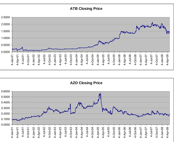
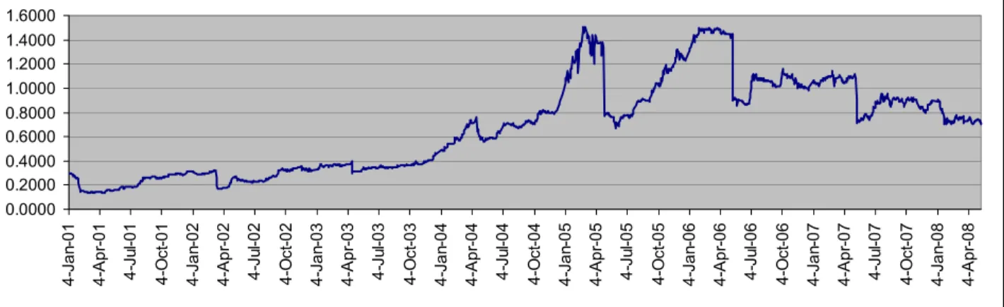
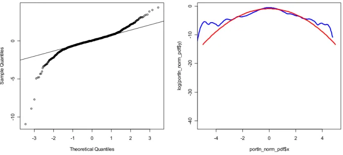
Daily closing prices for the three stocks, covering the period 4 Jan 2001 – 9 May 2008, were obtained from www.ktd.ro (financial information site of KTD Invest SA). The evolution of the closing prices for the stocks is shown in Fig. 1.

Then, logarithmic daily returns were computed for the three stocks and the portfolio, each data series consisting of 1814 observations. The evolution of the daily returns for each stock and for the portfolio during the analyzed period is shown in Fig. 2, while the descriptive statistics of the returns are presented in Table 1.

Fig. 1. The evolution of the closing prices for ATB, AZO and TLV

ATB Closing Price

0.0000 0.5000 1.0000 1.5000 2.0000 2.5000 4-Jan -01 4-A pr -01 4-Ju l-01 4-O ct -01 4-Jan -02 4-A pr -02 4-Ju l-02 4-O ct -02 4-Jan -03 4-A pr -03 4-Ju l-03 4-O ct -03 4-Jan -04 4-A pr -04 4-Ju l-04 4-O ct -04 4-Jan -05 4-A pr -05 4-Ju l-05 4-O ct -05 4-Jan -06 4-A pr -06 4-Ju l-06 4-O ct -06 4-Jan -07 4-A pr -07 4-Ju l-07 4-O ct -07 4-Jan -08 4-A pr -08

AZO Closing Price

0.0000 0.1000 0.2000 0.3000 0.4000 0.5000 0.6000 4-Jan -0 1 4-A p r-0 1 4-Ju l-01 4-O ct -01 4-Jan -0 2 4-A p r-0 2 4-Ju l-02 4-O ct -02 4-Jan -0 3 4-A p r-0 3 4-Ju l-03 4-O ct -03 4-Jan -0 4 4-A p r-0 4 4-Ju l-04 4-O ct -04 4-Jan -0 5 4-A p r-0 5 4-Ju l-05 4-O ct -05 4-Jan -0 6 4-A p r-0 6 4-Ju l-06 4-O ct -06 4-Jan -0 7 4-A p r-0 7 4-Ju l-07 4-O ct -07 4-Jan -0 8 4-A p r-0 8

(13)

TLV Closing Price 0.0000 0.2000 0.4000 0.6000 0.8000 1.0000 1.2000 1.4000 1.6000 4-Ja n-0 1 4-A p r-0 1 4-Ju l-01 4-O ct -0 1 4-Ja n-0 2 4-A p r-0 2 4-Ju l-02 4-O ct -0 2 4-Ja n-0 3 4-A p r-0 3 4-Ju l-03 4-O ct -0 3 4-Ja n-0 4 4-A p r-0 4 4-Ju l-04 4-O ct -0 4 4-Ja n-0 5 4-A p r-0 5 4-Ju l-05 4-O ct -0 5 4-Ja n-0 6 4-A p r-0 6 4-Ju l-06 4-O ct -0 6 4-Ja n-0 7 4-A p r-0 7 4-Ju l-07 4-O ct -0 7 4-Ja n-0 8 4-A p r-0 8

Fig. 2. The evolution of daily returns for ATB, AZO, TLV and the portfolio

Table 1. Descriptive statistics of daily returns

ATB AZO TLV PORTFOLIO

Logarithmic daily returns TLV

-0.7 -0.6 -0.5 -0.4 -0.3 -0.2 -0.1 0 0.1 0.2 0.3

Portfolio logarithmic daily returns

-0.25 -0.2 -0.15 -0.1 -0.05 0 0.05 0.1 0.15

Logarithmic daily returns ATB

-0.7 -0.6 -0.5 -0.4 -0.3 -0.2 -0.1 0 0.1 0.2 0.3

Logarithmic daily returns AZO

-0.7 -0.6 -0.5 -0.4 -0.3 -0.2 -0.1 0 0.1 0.2 0.3

(14)

Mean 0.001288686 0.000482618 0.000485777 0.00075236 Median 0 0 0 0.000692199 Maximum 0.139761942 0.247408173 0.095791065 0.092815783 Minimum -0.162166755 -0.669430654 -0.561469357 -0.230806724 St. Dev. 0.030788687 0.035601895 0.029359217 0.021086889 Skewness -0.496916313 -3.625751852 -7.962136836 -1.551673862 Kurtosis 12.46778119 77.47359745 128.567659 18.4562625

Skewness and kurtosis values of the series suggest that the stocks returns and also the portfolio returns aren't normally distributed (the empirical distributions are asymmetric to the left due to the negative skewness and they have a prominent peak due to the excess kurtosis). In order to verify the non-normality of the empirical distributions of the four returns series I used the Jarque-Bera test performed by Eviews. The test results, along with the histograms of the data series, are shown in Fig. 3 and indicate that the returns of the stocks and of the portfolio aren't normally distributed.

Fig. 3. Jarque-Bera test results and histograms for ATB, AZO, TLV and the portfolio

0 100 200 300 400 500 600 700 -0.15 -0.10 -0.05 0.00 0.05 0.10 Series: ATBLN Sample 1 1814 Observations 1814 Mean 0.001289 Median 0.000000 Maximum 0.139762 Minimum -0.162167 Std. Dev. 0.030789 Skewness -0.496505 Kurtosis 12.43840 Jarque-Bera 6807.749 Probability 0.000000 0 100 200 300 400 500 600 700 800 900 -0.50 -0.25 0.00 0.25 Series: AZOLN Sample 1 1814 Observations 1814 Mean 0.000483 Median 0.000000 Maximum 0.247408 Minimum -0.669431 Std. Dev. 0.035602 Skewness -3.622753 Kurtosis 77.26518 Jarque-Bera 420833.9 Probability 0.000000 0 200 400 600 800 1000 1200 -0.500 -0.375 -0.250 -0.125 0.000 Series: TLVLN Sample 1 1814 Observations 1814 Mean 0.000486 Median 0.000000 Maximum 0.095791 Minimum -0.561469 Std. Dev. 0.029359 Skewness -7.955551 Kurtosis 128.2185 Jarque-Bera 1204257. Probability 0.000000 0 100 200 300 400 500 -0.2 -0.1 0.0 0.1 Series: PORTLN Sample 1 1814 Observations 1814 Mean 0.000752 Median 0.000692 Maximum 0.092816 Minimum -0.230807 Std. Dev. 0.021087 Skewness -1.550390 Kurtosis 18.41039 Jarque-Bera 18676.25 Probability 0.000000

The four data series were also tested for the presence of the unit root using the Augmented Dickey-Fuller (ADF) performed in Eviews. The results are shown in Table 2 and, taking into

(15)

account that ADF test critical value for the 1% level is -3.433757, they lead to the conclusion that none of the data series has the unit root. The full results of the ADF test along with the test equations are given in the Appendix 1. Then, the correlation matrix of the raw returns was computed in Eviews and is shown in Table 3.

Table 2. ADF test results for daily returns of ATB, AZO, TLV and the portfolio Return series Value of t-statistic P value

ATB -24.32559 0 %

AZO -42.60324 0 %

TLV -37.72185 0 %

Portfolio -36.55895 0 %

Table 3. The correlation matrix of the raw returns

ATB AZO TLV ATB 1 0.176804 0.150407 AZO 0.176804 1 0.126762 TLV 0.150407 0.126762 1

The descriptive analysis of the primary data developed in this section leads to the following conclusions:

- The graphs of the returns show the presence of volatility clustering. This fact suggests that it would be better to compute VaR using conditional variance models, such as EWMA and GARCH models;

- The non-normality of the empirical distributions of the raw returns suggests that computing VaR with the quantiles of the standard normal distribution will tend to underestimate risk;

- The results of the ADF test allow us to consider that the mean and the variance of the data series are constant in time;

- The correlation coefficients, although positive, haven't high values so that the diversification effect is strong enough. Moreover, taking into account that former studies17 have documented a high average correlation inside emerging markets and the presence of a strong market factor, we may consider that the correlation coefficients in our case are very advantageous.

5. VaR using the historical volatility

(16)

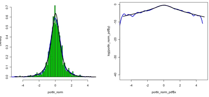
The portfolio returns were standardized using the historical mean and volatility of the sample. Because, generally, VaR is computed using the quantiles of the normal distribution I constructed three graphs (see Fig. 4) in order to visualize the non-normality of the standardized returns: the probability density function (PDF) of the empirical distribution, the QQ plot and the log PDF graph, all plotted against the standard normal distribution. Of course, from the previous section we already know that the portfolio returns aren't normally distributed and the situation doesn't change when they are standardized using their historical mean and volatility. So, the problem of non-normality is still to be dealt with.

Fig. 4. PDF of the empirical distribution, QQ plot and log PDF against the standard normal distribution Histogram of portln_norm portln_norm Den si ty -4 -2 0 2 4 0. 0 0. 1 0. 2 0. 3 0. 4 0. 5 0. 6 0. 7

(17)

-3 -2 -1 0 1 2 3 -1 0 -5 0 Normal Q-Q Plot Theoretical Quantiles S a mp le Q ua nti le s -4 -2 0 2 4 -4 0-30 -2 0-1 0 0 portln_norm_pdf$x log( por tln _n or m _p df $y )

In order to bypass this issue I estimated the parameters for three other distributions: t-Student (which allows for excess kurtosis), NIG and GH (which allow for skewness and excess kurtosis). The parameters were estimated through MLE using the Rmetrics package of the soft R. The results, along with the values for the informational criteria Akaike and Schwarz, are given in Table 4.

Table 4. Estimation results for t-Student, NIG and GH

t-Student Normal Inverse Gaussian Distribution General Hyperbolic Distribution alpha 0.72873077 alpha 0.24382855 beta -0.0394378 beta -0.03873113 degrees of freedom 8.724664 delta 0.67966102 delta 0.96331143 mu 0.03683542 mu 0.03825432 lambda -1.29956291

MLE -2453.487 MLE -2306.181 MLE -2302.68

AIC 2.7066 AIC 2.5471 AIC 2.5443

SIC 2.7092 SIC 2.5592 SIC 2.5595

Because the AIC and SIC values for NIG and GH are very close and the two criteria lead to different conclusions, both distributions were taken into account. Fig. 5 and Fig. 6 show the PDF of

(18)

the empirical distribution and log PDF against the estimated distributions NIG and GH (while the same graphs for the estimated t-Student distribution are given in Appendix 2).

Fig. 5. PDF of the empirical distribution and log PDF against the estimated NIG distribution

Histogram of portln_norm portln_norm De ns ity -4 -2 0 2 4 0. 0 0. 1 0. 2 0. 3 0. 4 0. 5 0. 6 0. 7 -4 -2 0 2 4 -4 0-3 0 -2 0-1 0 0 portln_norm_pdf$x log( por tln _n or m _pdf $y )

Fig. 6. PDF of the empirical distribution and log PDF against the estimated GH distribution

Histogram of portln_norm portln_norm De ns ity -4 -2 0 2 4 0. 0 0. 1 0. 2 0. 3 0. 4 0. 5 0. 6 0. 7 -4 -2 0 2 4 -4 0-3 0 -2 0-1 0 0 portln_norm_pdf$x log( por tln _n or m _pdf $y )

(19)

Analyzing these graphs it is clearly that NIG and GH fit much better the empirical distribution than does the standard normal distribution. Therefore, it would be reasonable to compute VaR using the quantiles of the NIG and GH distributions instead the ones of the standard normal distribution. The 1% quantiles for these distributions are given in Table 5.

Table 5. 1% quantiles for the standard normal distribution and estimated NIG and GH distributions

N Std. -2.326347 NIG -2.858291 GH -2.898633

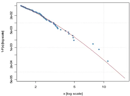
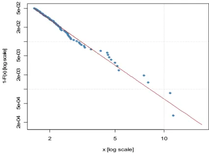
Another way of dealing with the non-normality of the standardized returns is the Extreme Value Theory (EVT). Using the Generalized Pareto Distribution (GPD), EVT models only the right tail of the distribution (the standardized returns in excess of a threshold) and because we are interested in extreme negative returns the EVT analysis is developed on the negative of returns. The threshold was set to be the 95 percentile of the sample of the standardized returns. The parameters of GPD were estimated through MLE and then the quantiles for VaR and Expected Shortfall (ES) were computed using the Rmetrics package of the soft R. The results are given in Table 6, while Fig. 7 shows the tail of the distribution along with the estimated GPD.

Table 6. Estimated parameters for GPD and the quantiles for VaR and ES according to EVT Parameter Estimates for GPD

xi 0.2575924 beta 0.8137205 Quantiles for VaR and ES for different probability levels according to EVT and N Std

Probability VaR EVT ES EVT N Std

1% 3.041225 4.701774 2.326347

0.5% 3.976777 5.961933 2.575831

0.1% 6.916062 9.921058 3.090253

0.05% 8.609074 12.20149 3.290560

0.01% 13.92812 19.36609 3.719090

(20)

2 5 10 5e-05 2e-04 1e-03 5e-03 2e-02

Tail of Underlying Distribution

x [log scale] 1-F( x) [l og sc al e]

The reason I included smaller quantiles than 1% and the standard normal distribution quantiles is that the normal and EVT distribution may lead to close values for 1% VaRs but very different 0.1% VaRs - for example - due to the different tail shapes. In such situations the risk profiles are very different and this is our case too. So, ES could be a better risk measure for our portfolio because it takes into consideration the shape of the tail.

At last, I also considered the Cornish-Fisher approach. It constructs approximation to quantiles using the skewness and excess kurtosis of the standardized returns. The result obtained for our data set is presented in Table 7.

Table 7. Cornish-Fisher approximation

Skewness -1.551673862 Excess Kurtosis 15.4562625 1% Q N Std -2.326347 1% CF -6.17468952

After modeling the distribution of the standardized returns and computing all the necessary quantiles, it was proceeded to the determination of VaR and ES. Using 750 days18 rolling mean and volatility I computed 1-day, 1% VaR for all the approaches considered above (except for the EVT approach where VaR and ES were computed for all of the specified quantiles) for the period 29 Jan

(21)

2004 – 9 May 200819. Also, historical VaR was computed as the 1% quantile of the series of the past 750 daily returns of the portfolio. The results obtained for VaR along with the negative of the returns of the portfolio (because VaR is a positive number) are shown in Fig. 8 and 9.

Fig. 8. 1-day, 1% VaR comparative graph

1-day, 1% VaR Comparative Graph

0 0.02 0.04 0.06 0.08 0.1 0.12 0.14 0.16 0.18 0.2 29/ 1/ 04 29/ 3/ 04 29/ 5/ 04 29/ 7/ 04 29/ 9/ 04 29/ 11/ 04 29/ 1/ 05 29/ 3/ 05 29/ 5/ 05 29/ 7/ 05 29/ 9/ 05 29/ 11/ 05 29/ 1/ 06 29/ 3/ 06 29/ 5/ 06 29/ 7/ 06 29/ 9/ 06 29/ 11/ 06 29/ 1/ 07 29/ 3/ 07 29/ 5/ 07 29/ 7/ 07 29/ 9/ 07 29/ 11/ 07 29/ 1/ 08 29/ 3/ 08 VaR N std VaR NIG VaR GHD Historical VaR -1*Port Return VaR CF approx

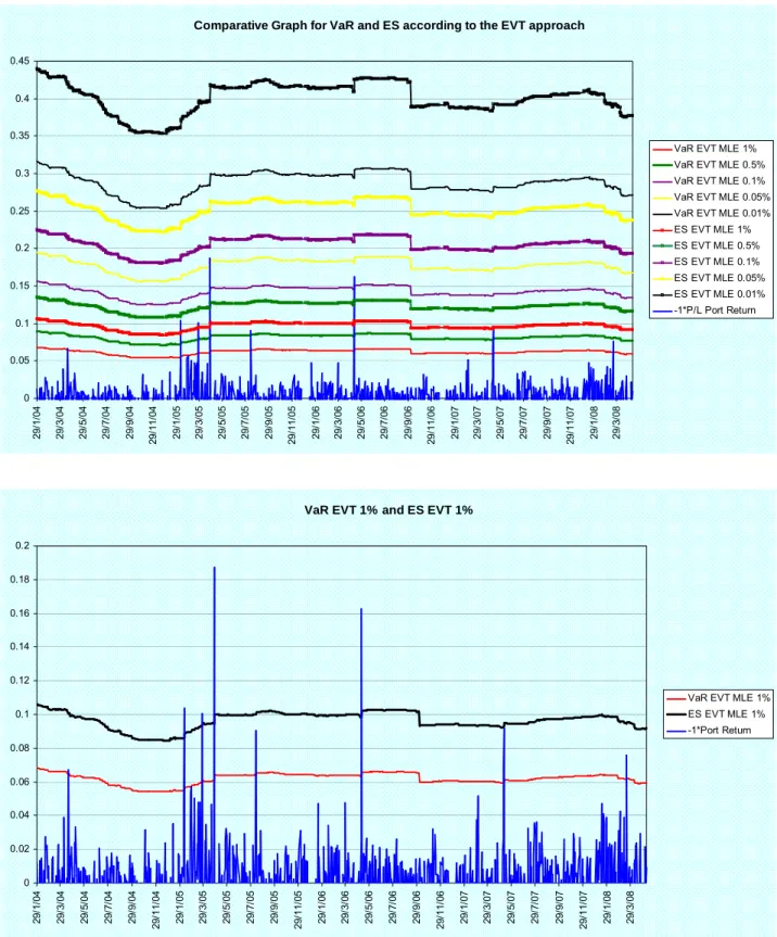
Fig. 9. 1-day VaR and ES for the EVT approach

(22)

Comparative Graph for VaR and ES according to the EVT approach 0 0.05 0.1 0.15 0.2 0.25 0.3 0.35 0.4 0.45 29/ 1/ 04 29/ 3/ 04 29/ 5/ 04 29/ 7/ 04 29/ 9/ 04 29/ 11/ 04 29/ 1/ 05 29/ 3/ 05 29/ 5/ 05 29/ 7/ 05 29/ 9/ 05 29/ 11/ 05 29/ 1/ 06 29/ 3/ 06 29/ 5/ 06 29/ 7/ 06 29/ 9/ 06 29/ 11/ 06 29/ 1/ 07 29/ 3/ 07 29/ 5/ 07 29/ 7/ 07 29/ 9/ 07 29/ 11/ 07 29/ 1/ 08 29/ 3/ 08

VaR EVT MLE 1% VaR EVT MLE 0.5% VaR EVT MLE 0.1% VaR EVT MLE 0.05% VaR EVT MLE 0.01% ES EVT MLE 1% ES EVT MLE 0.5% ES EVT MLE 0.1% ES EVT MLE 0.05% ES EVT MLE 0.01% -1*P/L Port Return

VaR EVT 1% and ES EVT 1%

0 0.02 0.04 0.06 0.08 0.1 0.12 0.14 0.16 0.18 0.2 29/ 1/ 04 29/ 3/ 04 29/ 5/ 04 29/ 7/ 04 29/ 9/ 04 29/ 11/ 04 29/ 1/ 05 29/ 3/ 05 29/ 5/ 05 29/ 7/ 05 29/ 9/ 05 29/ 11/ 05 29/ 1/ 06 29/ 3/ 06 29/ 5/ 06 29/ 7/ 06 29/ 9/ 06 29/ 11/ 06 29/ 1/ 07 29/ 3/ 07 29/ 5/ 07 29/ 7/ 07 29/ 9/ 07 29/ 11/ 07 29/ 1/ 08 29/ 3/ 08

VaR EVT MLE 1% ES EVT MLE 1% -1*Port Return

Table 8 shows if the computed risk measures match their respective critical levels (the term "errors %" denotes the percentage of the cases in which the portfolio loss exceeded VaR or ES) and

(23)

if the average ES indicators were exceeded by the average losses bigger than the corresponding VaR (marked with red if ES was exceeded).

Table 8. The precision of computed VaR and ES indicators

VaR Type VaR N Std VaR NIG VaR GHD VaR CF Historical VaR

Errors (%) 1.60% 1.03% 0.94% 0.19% 1.13%

VaR Type VaR EVT 1% VaR EVT 0.5% VaR EVT 0.1% VaR EVT 0.05% VaR EVT 0.01%

Errors (%) 0.85% 0.56% 0.19% 0.09% 0.00%

ES Type ES EVT 1% ES EVT 0.5% ES EVT 0.1% ES EVT 0.05% ES EVT 0.01%

Errors (%) 0.38% 0.19% 0.00% 0.00% 0.00%

Avg ES 0.096504267 0.122663027 0.204847737 0.252185694 0.400910516

Avg Loss

(> VaR) 0.105368373 0.122588525 0.174782102 0.187156452 0

The results reported here account for the following conclusions:

- VaR N Std, Historical VaR and VaR NIG don't match the critical level of 1% (although VaR NIG is very close) while VaR GHD and VaR CF pass the precision test (VaR CF obtaining a very good score, only 0.19% errors);

- Under the EVT approach only two VaRs, at 1% and 0.01%, match their critical levels, while all ES indicators pass the precision test (although ES 1% has a problem: on average it has a smaller value than the average of the losses exceeding VaR 1%).

Table 9. Capital requirements for VaRs 1% and ES 1% that passed the precision test VaR GHD VaR CF VaR EVT ES EVT Average value 0.059074122 0.127079491 0.06203409 0.096504267 Maximum 0.051504545 0.111509139 0.054116275 0.084531064 Minimum 0.064807013 0.139454722 0.068056092 0.1058931

If we are to choose between the 1% risk measures that passed the precision test VaR GHD would be the most appropriate because it provides the lowest level of capital coverage (see Table 9). The capital requirement is about 5.91% (average level) of the portfolio value (which is 1 RON in our case), while VaR EVT requires about 6.2%. VaR CF, although provides the best protection (only 0.19% errors), has the highest level of capital requirements being more expensive even than ES 1%.

(24)

6. VaR using the EWMA volatility model

In order to enhance the analysis of the risk measures developed in this study I considered time-varying volatility models. In this section it is used one of the simplest volatility models, namely the Exponentially Weighted Moving Average (EWMA) as developed by JP Morgan's RiskMetrics system. The model is written as

2 2 2 1 t (1 ) t t λσ λ R σ ₊ = + −

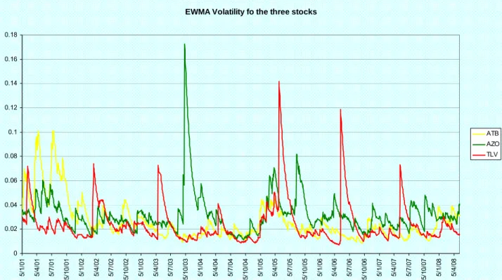
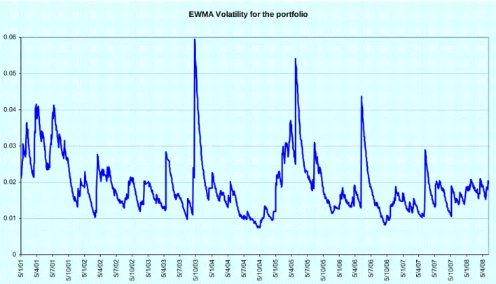
where λ < 1, σ denotes the volatility and R the return. Using this model I computed the volatility series for the three stocks considering that λ = 0.94 (the value set by RiskMetrics) and that the starting values are the historical standard deviations of the data series. Then, using the historical correlation coefficients, I computed the volatility series for the portfolio. The volatility graphs for the three stocks and for the portfolio are shown in Fig. 10.

Fig. 10. The EWMA Volatility of the three stocks and of the portfolio

EWMA Volatility fo the three stocks

0 0.02 0.04 0.06 0.08 0.1 0.12 0.14 0.16 0.18 5/ 1/ 01 5/ 4/ 01 5/ 7/ 01 5/ 10/ 01 5/ 1/ 02 5/ 4/ 02 5/ 7/ 02 5/ 10/ 02 5/ 1/ 03 5/ 4/ 03 5/ 7/ 03 5/ 10/ 03 5/ 1/ 04 5/ 4/ 04 5/ 7/ 04 5/ 10/ 04 5/ 1/ 05 5/ 4/ 05 5/ 7/ 05 5/ 10/ 05 5/ 1/ 06 5/ 4/ 06 5/ 7/ 06 5/ 10/ 06 5/ 1/ 07 5/ 4/ 07 5/ 7/ 07 5/ 10/ 07 5/ 1/ 08 5/ 4/ 08 ATB AZO TLV

(25)

EWMA Volatility for the portfolio 0 0.01 0.02 0.03 0.04 0.05 0.06 5/ 1/ 01 5/ 4/ 01 5/ 7/ 01 5/ 10/ 01 5/ 1/ 02 5/ 4/ 02 5/ 7/ 02 5/ 10/ 02 5/ 1/ 03 5/ 4/ 03 5/ 7/ 03 5/ 10/ 03 5/ 1/ 04 5/ 4/ 04 5/ 7/ 04 5/ 10/ 04 5/ 1/ 05 5/ 4/ 05 5/ 7/ 05 5/ 10/ 05 5/ 1/ 06 5/ 4/ 06 5/ 7/ 06 5/ 10/ 06 5/ 1/ 07 5/ 4/ 07 5/ 7/ 07 5/ 10/ 07 5/ 1/ 08 5/ 4/ 08

The returns of the stocks and of the portfolio were standardized using the historical mean and the computed EWMA volatility. The descriptive statistics for the series of the standardized returns are given in Table 10. The values for skewness and kurtosis indicate that we still have to face non-normality. The Jarque-Bera test applied to the standardized returns of the portfolio has a value of 15225.66 (with an associated p value of 0%) meaning they aren't normally distributed, while the ADF test confirms that the unit root is not present (the two tests are given in Appendix 3).

Table 10. Descriptive statistics of the returns standardized with EWMA volatility

Mean 0.022853282 0.008773423 0.01151103 0.015033927 Median -0.062906618 -0.016700982 -0.023587187 -0.004146442 Maximum 6.66875623 10.1983607 7.288494731 7.380381514 Minimum -5.677694158 -11.92240587 -47.57183779 -11.35463294 Std. Dev. 1.077012211 1.14691887 1.658327606 1.160841498 Skewness 0.570426272 0.223325423 -15.01802686 -1.105297369 Kurtosis 7.912768016 20.12699426 396.8349199 17.0621412

In order to visualize the non-normality of the portfolio standardized returns Fig. 11 shows three graphs: the probability density function (PDF) of the empirical distribution, the QQ plot and the log PDF graph, all plotted against the standard normal distribution.

(26)

Fig. 11. PDF of the empirical distribution, QQ plot and log PDF against the standard normal distribution Histogram of portln_norm portln_norm Den si ty -4 -2 0 2 4 0. 0 0. 1 0. 2 0. 3 0. 4 0. 5 0. 6 -3 -2 -1 0 1 2 3 -1 0 -5 0 5 Normal Q-Q Plot Theoretical Quantiles S a m p le Q ua nt ile s -4 -2 0 2 4 -3 0 -2 0 -1 0 0 portln_norm_pdf$x log( por tln _n or m _pdf $y )

As in the previous section, the first way to deal with the non-normality of the data was to estimate the parameters for t-Student, NIG and GH distributions. The parameters were estimated through MLE using the Rmetrics package of the soft R. The results, along with the values for the informational criteria Akaike and Schwarz, are given in Table 11.

(27)

t-Student Normal Inverse Gaussian Distribution General Hyperbolic Distribution alpha 0.71864289 alpha 0.01319607 beta -0.01048403 beta -0.01318189 degrees of freedom 6.32333 delta 0.89238534 delta 1.38629802 mu 0.0280556 mu 0.03261598 lambda -1.72038174

MLE -2656.422 MLE -2611.03 MLE -2603.462

AIC 2.9299 AIC 2.8832 AIC 2.8759

SIC 2.9329 SIC 2.8953 SIC 2.8911

Because the AIC and SIC values for NIG and GH are very close both distributions were taken into account. Fig. 12 and Fig. 13 show the PDF of the empirical distribution and log PDF against the estimated distributions NIG and GH (while the same graphs for the estimated t-Student distribution are given in Appendix 3). Analyzing these graphs it is clearly that NIG and GH fit much better the empirical distribution than does the standard normal distribution. Therefore, it would be reasonable to compute VaR using the quantiles of the NIG and GH distributions instead the ones of the standard normal distribution. The 1% quantiles for these distributions are given in Table 12.

Histogram of portln_norm portln_norm De ns ity -4 -2 0 2 4 0. 0 0. 1 0. 2 0. 3 0. 4 0. 5 0. 6 -4 -2 0 2 4 -3 0 -2 0 -1 0 0 portln_norm_pdf$x log( por tln _n or m _pdf $y )

(28)

Fig. 13. PDF of the empirical distribution and log PDF against the estimated GH distribution Histogram of portln_norm portln_norm De ns ity -4 -2 0 2 4 0. 0 0. 1 0. 2 0. 3 0. 4 0. 5 0. 6 -4 -2 0 2 4 -3 0 -2 0 -1 0 0 portln_norm_pdf$x log( por tln _n or m _pdf $y )

N Std. -2.326347 NIG -3.134162 GH -3.098957

As in the previous section, I used also the EVT approach in order to deal with the non-normality of the standardized data. Again, the threshold was set to be the 95 percentile of the sample of the standardized returns while the parameters of GPD were estimated through MLE and then the quantiles for VaR and ES were computed using Rmetrics. The results are given in Table 13, while Fig. 14 shows the tail of the distribution along with the estimated GPD.

xi 0.4300091 beta 0.64173

Quantiles for VaR and ES for different probability levels according to EVT and N Std

1% 3.100416 5.352915 2.326347

0.5% 4.137198 7.171859 2.575831

0.1% 8.151101 14.213906 3.090253

0.05% 10.941692 19.109759 3.290560

(29)

Fig. 14. The tail of the distribution along with the estimated GDP 2 5 10 2e -04 5e-04 2e-03 5e-03 2e-02 5e-02

x [log scale] 1-F (x ) [ log sc al e]

We observe the same situation as in the previous section: the quantiles of the normal and EVT distribution are very different for probabilities below 1% due to the different tail shapes. Therefore, the risk profiles are very different and ES could be a better risk measure for our portfolio because it takes into consideration the shape of the tail.

At last, the Cornish-Fisher approach was also considered. The approximation for the 1% quantile, computed using the skewness and excess kurtosis of the returns standardized with the EWMA volatility, is given in Table 14.

Skewness -1.105297369 Excess Kurtosis 14.0621412 1% Q N Std -2.326347 1% CF -5.966873733

After modeling the distribution of the standardized returns and computing all the necessary quantiles, it was proceeded to the determination of VaR and ES. Using the EWMA volatility I computed 1-day, 1% VaR for all the approaches considered above (except for the EVT approach where VaR and ES were computed for all of the specified quantiles) for the period 29 Jan 2004 – 9 May 2008. Also, historical VaR was computed using the 1% quantile of the series of the past 750

(30)

daily standardized returns of the portfolio. The results obtained for VaR along with the negative of the returns of the portfolio (because VaR is a positive number) are shown in Fig. 15 and 16. Table 15 shows if the computed risk measures match their respective critical levels (the term "errors %" denotes the percentage of the cases in which the portfolio loss exceeded VaR or ES) and if the average ES indicators were exceeded by the average losses bigger than the corresponding VaR (marked with red if ES was exceeded).

Errors (%) 2.26% 1.03% 1.13% 0.19% 1.41%

Errors (%) 1.13% 0.75% 0.09% 0.09% 0.00%

Errors (%) 0.19% 0.09% 0.00% 0.00% 0.00%

Avg ES 0.092887278 0.124823403 0.248464206 0.334423189 0.66721369

Avg Loss

(> VaR) 0.085960761 0.106005833 0.162407753 0.162407753 0

Fig. 15. 1-day, 1% VaR EWMA comparative graph

1-day, 1% VaR EWMA Comparative Graph

0 0.05 0.1 0.15 0.2 0.25 0.3 29 /1/ 04 29 /3/ 04 29 /5/ 04 29 /7/ 04 29 /9/ 04 29/ 11/ 04 29 /1/ 05 29 /3/ 05 29 /5/ 05 29 /7/ 05 29 /9/ 05 29/ 11/ 05 29 /1/ 06 29 /3/ 06 29 /5/ 06 29 /7/ 06 29 /9/ 06 29/ 11/ 06 29 /1/ 07 29 /3/ 07 29 /5/ 07 29 /7/ 07 29 /9/ 07 29/ 11/ 07 29 /1/ 08 29 /3/ 08 VaR EWMA N std VaR EWMA NIG VaR EWMA GHD Historical VaR EWMA -1*Port Return VaR EWMA CFapprox

(31)

Fig. 16. 1-day VaR EWMA for the EVT approach

Comparative Graph for VaR EWMA according to the EVT approach

0 0.1 0.2 0.3 0.4 0.5 0.6 29/ 1/ 04 29/ 3/ 04 29/ 5/ 04 29/ 7/ 04 29/ 9/ 04 29/ 11/ 04 29/ 1/ 05 29/ 3/ 05 29/ 5/ 05 29/ 7/ 05 29/ 9/ 05 29/ 11/ 05 29/ 1/ 06 29/ 3/ 06 29/ 5/ 06 29/ 7/ 06 29/ 9/ 06 29/ 11/ 06 29/ 1/ 07 29/ 3/ 07 29/ 5/ 07 29/ 7/ 07 29/ 9/ 07 29/ 11/ 07 29/ 1/ 08 29/ 3/ 08

VaR EWMA EVT MLE 1% VaR EWMA EVT MLE 0.5% VaR EWMA EVT MLE 0.1% VaR EWMA EVT MLE 0.05% -1*Port Return

VaR EWMA EVT 1% and ES EWMA 1%

0 0.05 0.1 0.15 0.2 0.25 0.3 29/ 1/ 04 29/ 3/ 04 29/ 5/ 04 29/ 7/ 04 29/ 9/ 04 29/ 11/ 04 29/ 1/ 05 29/ 3/ 05 29/ 5/ 05 29/ 7/ 05 29/ 9/ 05 29/ 11/ 05 29/ 1/ 06 29/ 3/ 06 29/ 5/ 06 29/ 7/ 06 29/ 9/ 06 29/ 11/ 06 29/ 1/ 07 29/ 3/ 07 29/ 5/ 07 29/ 7/ 07 29/ 9/ 07 29/ 11/ 07 29/ 1/ 08 29/ 3/ 08

VaR EWMA EVT MLE 1% ES EWMA EVT MLE 1% -1*Port Return

(32)

- VaR N Std, Historical VaR, VaR NIG and VaR GHD didn't succeed in matching the critical level of 1% (although VaR NIG is very close), only VaR CF being able to pass the precision test with the same score as in the previous section;

- Under the EVT approach only two VaRs, at 0.1% and 0.01%, match their critical levels, but all ES indicators pass the precision test;

- It seems that the EWMA volatility model tends to underestimate risk for the portfolio and the period analyzed in my study, the results for the 1% risk measures being worse than in the case of using historical volatility (see the previous section).

Table 16. Capital requirements for VaR CF 1% and ES 1%

VaR CF 1% ES EVT 1% Average value 0.103666864 0.092887278 Maximum 0.042467889 0.037951806 Minimum 0.326926586 0.293116434

If we are to choose between VaR CF and ES (these being the only 1% risk measures that passed the precision test), ES 1% would be the most appropriate because it provides the lowest level of capital coverage (see Table 16). The capital requirement is about 9.29% (average level) of the portfolio value, while VaR CF requires about 10.37%. Moreover, the two risk measures offer the same accuracy, namely 0.19% errors.

7. VaR using a GARCH volatility model for portfolio returns

The analysis developed in this study was further improved by considering GARCH volatility models which overrun some of the shortcomings of EWMA model. First, I considered the simplest case: a GARCH (1,1) volatility model for the portfolio returns which has the advantage that few calculations are needed even in the case of large portfolios. The model is written as

2 2 2 1 t t t ω αR βσ σ ₊ = + +

(where α + β < 1, σ denotes the volatility, R the return) and the parameters α, β and ω were estimated through MLE in Eviews. With the estimated values of the parameters I computed the volatility series of the portfolio returns using as starting value the historical standard deviation. The

(33)

results of the estimation are given in Table 17 (for the full results see Appendix 4) while Fig. 17 shows the graph of the GARCH volatility of the portfolio during the analyzed period.

Table 17. GARCH (1,1) volatility model for the portfolio returns

ω

0.00003674

α

0.23330744

β

0.73422658 Fig. 17. The GARCH Volatility of the portfolio

The GARCH volatility of the portfolio

0 0.02 0.04 0.06 0.08 0.1 0.12 5/ 1/ 01 5/ 4/ 01 5/ 7/ 01 5/ 10/ 01 5/ 1/ 02 5/ 4/ 02 5/ 7/ 02 5/ 10/ 02 5/ 1/ 03 5/ 4/ 03 5/ 7/ 03 5/ 10/ 03 5/ 1/ 04 5/ 4/ 04 5/ 7/ 04 5/ 10/ 04 5/ 1/ 05 5/ 4/ 05 5/ 7/ 05 5/ 10/ 05 5/ 1/ 06 5/ 4/ 06 5/ 7/ 06 5/ 10/ 06 5/ 1/ 07 5/ 4/ 07 5/ 7/ 07 5/ 10/ 07 5/ 1/ 08 5/ 4/ 08

The returns of the portfolio were standardized using the historical mean and the computed GARCH volatility. The descriptive statistics for the series of the standardized returns are given in Table 18. The values for skewness and kurtosis indicate that we still have to face non-normality. The Jarque-Bera test applied to the standardized returns of the portfolio has a value of 25590.53 (with an associated p value of 0%) meaning they aren't normally distributed, while the ADF test confirms that the unit root is not present (the two tests are given in Appendix 4).

(34)

Table 18. Descriptive statistics of the portfolio returns standardized with GARCH volatility PORTFOLIO Mean 0.002768796 Median -0.00332796 Maximum 5.807380535 Minimum -10.0040107 Std. Dev. 1.001248131 Skewness -1.513391092 Kurtosis 20.07196361

Similarly to the previous sections, the first way to deal with the non-normality of the data was to estimate the parameters for t-Student, NIG and GH distributions. The parameters were estimated through MLE using the Rmetrics package of the soft R. The results, along with the values for the informational criteria Akaike and Schwarz, are given in Table 19.

Fig. 18. PDF of the empirical distribution, QQ plot and log PDF against the standard normal distribution Histogram of portln_norm portln_norm Den si ty -4 -2 0 2 4 0. 0 0. 1 0. 2 0 .3 0 .4 0. 5 0. 6 0. 7

(35)

-3 -2 -1 0 1 2 3 -1 0 -5 0 5 Normal Q-Q Plot Theoretical Quantiles S a mp le Q ua nti le s -4 -2 0 2 4 -4 0-3 0 -2 0-1 0 0 portln_norm_pdf$x lo g( por tln _n or m _pdf $y )

t-Student Normal Inverse

Gaussian Distribution General Hyperbolic Distribution alpha 0.94278975 alpha 0.05570423 beta -0.05636764 beta -0.05570417 degrees of freedom 9.6544 delta 0.84625444 delta 1.32257003 mu 0.05345637 mu 0.054024 lambda -1.94888169

MLE -2451.553 MLE -2350.707 MLE -2338.908

AIC 2.704 AIC 2.5961 AIC 2.5842

SIC 2.7071 SIC 2.6083 SIC 2.5994

Because the AIC and SIC values for NIG and GH are very close both distributions were taken into account. Fig. 19 and Fig. 20 show the PDF of the empirical distribution and log PDF against the estimated distributions NIG and GH (while the same graphs for the estimated t-Student distribution are given in Appendix 4).

(36)

Fig. 19. PDF of the empirical distribution and log PDF against the estimated NIG distribution Histogram of portln_norm portln_norm De ns ity -4 -2 0 2 4 0. 0 0. 1 0. 2 0. 3 0. 4 0. 5 0. 6 0. 7 -4 -2 0 2 4 -4 0 -3 0 -2 0 -1 0 0 portln_norm_pdf$x log( por tln _n or m _pdf $y )

Fig. 20. PDF of the empirical distribution and log PDF against the estimated GH distribution

Histogram of portln_norm portln_norm De ns ity -4 -2 0 2 4 0. 0 0. 1 0. 2 0. 3 0. 4 0. 5 0. 6 0. 7 -4 -2 0 2 4 -4 0 -3 0 -2 0 -1 0 0 portln_norm_pdf$x log( por tln _n or m _p df $y )

Analyzing these graphs it is clearly that NIG and GH fit much better the empirical distribution than does the standard normal distribution. Therefore, it would be reasonable to compute VaR using the quantiles of the NIG and GH distributions instead the ones of the standard normal distribution. The 1% quantiles for these distributions are given in Table 20.

(37)

N Std. -2.326347 NIG -2.699688 GH -2.658805

As in the previous sections, I used also the EVT approach in order to deal with the non-normality of the standardized data. Again, the threshold was set to be the 95 percentile of the sample of the standardized returns while the parameters of GPD were estimated through MLE and then the quantiles for VaR and ES were computed using Rmetrics. The results are given in Table 21, while Fig. 21 shows the tail of the distribution along with the estimated GPD.

xi 0.4301966 beta 0.5696852 Quantiles for VaR and ES for different probability levels according to EVT and N Std

1% 2.691543 4.692425 2.326347

0.5% 3.61227 6.308292 2.575831

0.1% 7.177687 12.565568 3.090253

0.05% 9.656977 16.9167 3.290560

0.01% 19.257766 33.766002 3.719090

Fig. 21. The tail of the distribution along with the estimated GDP

2 5 10 2e-04 5e -04 2e-03 5e -0 3 2e-02 5e-02

x [log scale] 1-F( x) [l og s ca le ]

(38)

We observe the same situation as in the previous sections: the quantiles of the normal and EVT distribution are very different for probabilities below 1% due to the different tail shapes. Therefore, the risk profiles are significantly different and ES could be a better risk measure for our portfolio because it takes into consideration the shape of the tail.

At last, the Cornish-Fisher approach was also considered. The approximation for the 1% quantile, computed using the skewness and excess kurtosis of the returns standardized with the GARCH volatility, is given in Table 22.

Skewness -1.513391092 Excess Kurtosis 17.07196361 1% Q N Std -2.326347 1% CF _-6.56842902

After modeling the distribution of the standardized returns and computing all the necessary quantiles, it was proceeded to the determination of VaR and ES. Using the GARCH volatility I computed 1-day, 1% VaR for all the approaches considered above (except for the EVT approach where VaR and ES were computed for all of the specified quantiles) for the period 29 Jan 2004 – 9 May 2008. Also, historical VaR was computed using the 1% quantile of the series of the past 750 daily standardized returns of the portfolio. The results obtained for VaR along with the negative of the returns of the portfolio (because VaR is a positive number) are shown in Fig. 22 and 23. Table 23 shows if the computed risk measures match their respective critical levels (the term "errors %" denotes the percentage of the cases in which the portfolio loss exceeded VaR or ES) and if the average ES indicators were exceeded by the average losses bigger than the corresponding VaR (marked with red if ES was exceeded).

Errors (%) 1.79% 0.94% 0.94% 0.19% 1.22%

Errors (%) 0.94% 0.47% 0.19% 0.09% 0.00%

Errors (%) 0.28% 0.19% 0.00% 0.00% 0.00%

Avg ES 0.094189578 0.127001983 0.25406459 0.342420319 0.684568603

Avg Loss

(39)

Fig. 22. 1-day, 1% VaR GARCH comparative graphs

1-day, 1% VaR GARCH Comparative Graph

0 0.1 0.2 0.3 0.4 0.5 0.6 29/ 1/ 04 29/ 3/ 04 29/ 5/ 04 29/ 7/ 04 29/ 9/ 04 29/ 11/ 04 29/ 1/ 05 29/ 3/ 05 29/ 5/ 05 29/ 7/ 05 29/ 9/ 05 29/ 11/ 05 29/ 1/ 06 29/ 3/ 06 29/ 5/ 06 29/ 7/ 06 29/ 9/ 06 29/ 11/ 06 29/ 1/ 07 29/ 3/ 07 29/ 5/ 07 29/ 7/ 07 29/ 9/ 07 29/ 11/ 07 29/ 1/ 08 29/ 3/ 08 VaR GARCH N std VaR GARCH NIG -1*Port Return VaR GARCH CF

1-day, 1% VaR GARCH Comparative Graph

0 0.05 0.1 0.15 0.2 0.25 29/ 1/ 04 29/ 3/ 04 29/ 5/ 04 29/ 7/ 04 29/ 9/ 04 29/ 11/ 04 29/ 1/ 05 29/ 3/ 05 29/ 5/ 05 29/ 7/ 05 29/ 9/ 05 29/ 11/ 05 29/ 1/ 06 29/ 3/ 06 29/ 5/ 06 29/ 7/ 06 29/ 9/ 06 29/ 11/ 06 29/ 1/ 07 29/ 3/ 07 29/ 5/ 07 29/ 7/ 07 29/ 9/ 07 29/ 11/ 07 29/ 1/ 08 29/ 3/ 08 VaR GARCH GHD Historical VaR GARCH -1*Port Return

(40)

Fig. 23. 1-day VaR GARCH for the EVT approach

Comparative graph for VaR GARCH according to EVT approach

0 0.1 0.2 0.3 0.4 0.5 0.6 0.7 29/ 1/ 04 29/ 3/ 04 29/ 5/ 04 29/ 7/ 04 29/ 9/ 04 29/ 11/ 04 29/ 1/ 05 29/ 3/ 05 29/ 5/ 05 29/ 7/ 05 29/ 9/ 05 29/ 11/ 05 29/ 1/ 06 29/ 3/ 06 29/ 5/ 06 29/ 7/ 06 29/ 9/ 06 29/ 11/ 06 29/ 1/ 07 29/ 3/ 07 29/ 5/ 07 29/ 7/ 07 29/ 9/ 07 29/ 11/ 07 29/ 1/ 08 29/ 3/ 08

VaR EVT MLE 1% VaR EVT MLE 0.5% VaR EVT MLE 0.1% -1*Port Return

VaR GARCH EVT 1% and ES EVT 1%

0 0.05 0.1 0.15 0.2 0.25 0.3 0.35 0.4 0.45 29/ 1/ 04 29/ 3/ 04 29/ 5/ 04 29/ 7/ 04 29/ 9/ 04 29/ 11/ 04 29/ 1/ 05 29/ 3/ 05 29/ 5/ 05 29/ 7/ 05 29/ 9/ 05 29/ 11/ 05 29/ 1/ 06 29/ 3/ 06 29/ 5/ 06 29/ 7/ 06 29/ 9/ 06 29/ 11/ 06 29/ 1/ 07 29/ 3/ 07 29/ 5/ 07 29/ 7/ 07 29/ 9/ 07 29/ 11/ 07 29/ 1/ 08 29/ 3/ 08

VaR EVT MLE 1% ES EVT MLE 1% -1*Port Return

(41)

The results reported here account for the following conclusions:

- VaR N Std and Historical VaR didn't succeed in matching the critical level of 1%, while VaR NIG, VaR GHD and VaR CF passed the precision test, VaR CF having the best score as in the previous sections;

- Under the EVT approach three VaRs, at 1%, 0.5% and 0.01%, match their critical levels, while all ES indicators pass the precision test (although ES 1% has a problem: on average it has a smaller value than the average of the losses exceeding VaR EVT 1%);

- It seems that using the GARCH volatility model for the portfolio returns improved the risk measures analyzed in this study, these being the best results so far.

Table 24. Capital requirements for VaRs 1% and ES 1% that passed the precision test VaR NIG 1% VaR GHD 1% VaR CF 1% VaR EVT 1% ES EVT 1% Average value 0.053724308 0.052894123 0.132284423 0.053558913 0.094189578 Maximum 0.031672086 0.031168008 0.079372735 0.03157166 0.056242055 Minimum 0.246993774 0.243228204 0.603328119 0.246243571 0.430536852

If we are to choose between the 1% risk measures that passed the precision test VaR GHD would be the most appropriate because it provides the lowest level of capital coverage (see Table 24). The capital requirement is about 5.29% (average level) of the portfolio value while VaR EVT requires about 5.36% and VaR NIG about 5.37%. VaR CF, as it has been already seen in the previous sections, has the highest level of capital requirement being more expensive even than ES 1%.

8. VaR using GARCH volatility models for the stock returns

In this stage GARCH models were considered for the volatility of each stock returns. Therefore, I estimated GARCH (1,1) models for ATB and AZO, while for TLV a TARCH (1,1) was estimated. The specification of the models was established taking into account the results obtained at the autocorrelation tests of the residuals and of the squared residuals. Also, I verified that the sum of ARCH and GARCH coefficients is below 1. The parameters of the three models were estimated through MLE in Eviews. On the basis of estimation results I computed the volatility series for the three stocks considering that the starting values are the historical standard deviations of the data series. Then, using the historical correlation coefficients, I computed the volatility series

(42)

for the portfolio. The results of the estimation are given in Table 25 (for the full results see Appendix 5) while Fig. 24 shows the volatility graphs for the three stocks and for the portfolio.

Table 25. Estimation results for the volatility of the stock returns

GARCH (1,1) ATB GARCH (1,1) AZO TARCH (1,1) TLV

ω

0.000021415 0.000067782 0.000043996

α

0.124995782 0.097710524 1.869205806

β

0.851955326 0.857306946 0.561647124

λ

- - -1.566882386

The returns of the stocks and of the portfolio were standardized using the historical mean and the computed GARCH volatility. The descriptive statistics for the series of the standardized returns are given in Table 26. The values for skewness and kurtosis indicate that we still have to face non-normality. The Jarque-Bera test applied to the standardized returns of the portfolio has a value of 14846.91 (with an associated p value of 0%) meaning they aren't normally distributed, while the ADF test confirms that the unit root is not present (the two tests are given in Appendix 5).

Fig. 24. The GARCH Volatility of the three stocks and of the portfolio

GARCH volatility for the three stocksi

-0.03 0.02 0.07 0.12 0.17 0.22 0.27 0.32 5/ 1/ 01 5/ 4/ 01 5/ 7/ 01 5/ 10/ 01 5/ 1/ 02 5/ 4/ 02 5/ 7/ 02 5/ 10/ 02 5/ 1/ 03 5/ 4/ 03 5/ 7/ 03 5/ 10/ 03 5/ 1/ 04 5/ 4/ 04 5/ 7/ 04 5/ 10/ 04 5/ 1/ 05 5/ 4/ 05 5/ 7/ 05 5/ 10/ 05 5/ 1/ 06 5/ 4/ 06 5/ 7/ 06 5/ 10/ 06 5/ 1/ 07 5/ 4/ 07 5/ 7/ 07 5/ 10/ 07 5/ 1/ 08 5/ 4/ 08 ATB AZO TLV

(43)

GARCH volatility for the portfolio 0 0.02 0.04 0.06 0.08 0.1 0.12 5/ 1/ 01 5/ 4/ 01 5/ 7/ 01 5/ 10/ 01 5/ 1/ 02 5/ 4/ 02 5/ 7/ 02 5/ 10/ 02 5/ 1/ 03 5/ 4/ 03 5/ 7/ 03 5/ 10/ 03 5/ 1/ 04 5/ 4/ 04 5/ 7/ 04 5/ 10/ 04 5/ 1/ 05 5/ 4/ 05 5/ 7/ 05 5/ 10/ 05 5/ 1/ 06 5/ 4/ 06 5/ 7/ 06 5/ 10/ 06 5/ 1/ 07 5/ 4/ 07 5/ 7/ 07 5/ 10/ 07 5/ 1/ 08 5/ 4/ 08

Table 26. Descriptive statistics of the returns standardized with GARCH volatility

Mean 0.019232517 0.001177774 0.01391282 -0.000723316 Median -0.062499878 -0.015806861 -0.018987492 -0.003431596 Maximum 7.417686382 9.720063979 4.671654838 6.354261631 Minimum -6.730922299 -11.5023275 -15.75192717 -9.728993413 Std. Dev. 1.004357344 0.999613558 0.951366414 0.986031755 Skewness 0.451135773 -0.339593675 -5.088694033 -1.246870005 Kurtosis 8.954522622 22.91252826 72.92644788 16.83352693

(44)

Fig. 25. PDF of the empirical distribution, QQ plot and log PDF against the standard normal distribution Histogram of portln_norm portln_norm De ns ity -4 -2 0 2 4 0 .00 .1 0. 20 .3 0 .40 .5 0. 60 .7 -3 -2 -1 0 1 2 3 -1 0 -5 0 5 Normal Q-Q Plot Theoretical Quantiles S a m p le Q ua nt ile s -4 -2 0 2 4 -4 0 -3 0 -2 0 -1 0 0 portln_norm_pdf$x lo g( por tln _n or m _pdf $y )

Similarly to the previous sections, the first way to deal with the non-normality of the data was to estimate the parameters for t-Student, NIG and GH distributions. The parameters were estimated through MLE using the Rmetrics package of the soft R. The results, along with the values for the informational criteria Akaike and Schwarz, are given in Table 27.

(45)

t-Student Normal Inverse

Gaussian Distribution General Hyperbolic Distribution alpha 0.98043236 alpha 0.06596887 beta -0.06929081 beta -0.06596871 degrees of freedom 10.47379 delta 0.87046629 delta 1.37267037 mu 0.06095307 mu 0.05925987 lambda -2.03883398

MLE -2449.394 MLE -2353.705 MLE -2344.757

AIC 2.7016 AIC 2.5995 AIC 2.5907

SIC 2.7047 SIC 2.6116 SIC 2.6059

Because the AIC and SIC values for NIG and GH are very close both distributions were taken into account. Fig. 26 and Fig. 27 show the PDF of the empirical distribution and log PDF against the estimated distributions NIG and GH (while the same graphs for the estimated t-Student distribution are given in Appendix 5). Analyzing these graphs it is clearly that NIG and GH fit much better the empirical distribution than does the standard normal distribution. Therefore, it would be reasonable to compute VaR using the quantiles of the NIG and GH distributions instead the ones of the standard normal distribution. The 1% quantiles for these distributions are given in Table 28.

Histogram of portln_norm portln_norm De ns ity -4 -2 0 2 4 0 .00 .1 0. 20 .3 0 .40 .5 0 .60 .7 -4 -2 0 2 4 -4 0 -3 0 -2 0 -1 0 0 portln_norm_pdf$x lo g( por tln _n or m _pdf $y )