Camera Localization Using
Trajectories and Maps
Raúl Mohedano, Andrea Cavallaro, and Narciso García
Abstract—We propose a new Bayesian framework for automatically determining the position (location and orientation) of an uncalibrated camera using the observations of moving objects and a schematic map of the passable areas of the environment. Our approach takes advantage of static and dynamic information on the scene structures through prior probability distributions for object dynamics. The proposed approach restricts plausible positions where the sensor can be located while taking into account the inherent ambiguity of the given setting. The proposed framework samples from the posterior probability distribution for the camera position via data driven MCMC, guided by an initial geometric analysis that restricts the search space. A Kullback-Leibler divergence analysis is then used that yields the final camera position estimate, while explicitly isolating ambiguous settings. The proposed approach is evaluated in synthetic and real environments, showing its satisfactory performance in both ambiguous and unambiguous settings.
Index Terms—Vision and scene understanding, camera calibration, Markov processes, tracking
1 INTRODUCTION
V
ISUAL-BASED camera self-positioning is fundamental for automatic vehicle guidance, aerial imaging, photo-grammetry and calibration of previously placed cameras (e.g., CCTV networks). Existing methods use general geo-m e t r i c / d y n a geo-m i c assugeo-mptions without any knowledge of the site being observed, or use specific environmental knowledge (e.g., in the form of a map). Visual observation of invariants that are i n d e p e n d e n t from the specific camera location can be used for camera position estimation [1], [2]: for instance, the observation of stars [3], vertical lines and vanishing points of architectural structures [4] can be used to infer sensor orientation, w i t h o u t providing camera loca-tion estimaloca-tions. Alternatively, trajectory models can also be used for extrinsic parameter calibration of camera net-works [5], [6], [7], [8] and for temporal synchronization [9], [10]. Regular object dynamics such as polynomials of k n o w n degree [11] and probabilistic linear Markov models [12], [13] are generally a s s u m e d to allow the estimation of relative sensor positions from reconstructed trajectories inside and outside the field of view (FoV) of the cameras.Most works that use environmental knowledge assume prior information obtained offline. Only certain Simulta-neous Localization A n d M a p p i n g (SLAM) systems build online 3D descriptions for sequential re-localization [14], [15]. There are however SLAM approaches that use 3D scene models to match the inferred 3D models to improve
the robustness a n d accuracy of the resulting positioning [16], [17]. Direct image registration between the camera's FoV and a n aerial/satellite m a p of the site u n d e r s t u d y [18] is a valid option w i t h planar environments or aerial cam-eras. Matching approximate observations of environmental landmarks of the ground-plane of the scene a n d their actual positions on the street m a p assumes m a n u a l user interac-tion [19], or automatic feature extracinterac-tion from b o t h satellite and camera views [20]. A more versatile approach b u t less accurate and more d e m a n d i n g in terms of m a p size and processing uses geo-referenced street view data sets (such as Google Street View or OpenStreetMap) for absolute cam-era positioning [21], [22].
In this paper, w e present a Bayesian framework for infer-ring, from the observed trajectories of moving objects a n d a schematic m a p of the scene indicating passable areas of the environment, the absolute location a n d orientation (i.e., position) of a fixed camera w h o s e view of the dominant ground-plane of the scene is a s s u m e d metrically rectified. We consider prior probability distributions for object trajec-tories taking into account the dynamics encouraged by the structures defined in the m a p of the specific scene, a n d com-pare them to the 2D tracks to obtain the posterior probabil-ity distribution for the camera position. This posterior is analyzed using Monte Carlo probabilistic sampling and Kullback-Liebler divergence-based clustering to obtain the final estimation for the given setting. It is important to note that, unlike existing visual positioning systems that do not perform any reliability analysis [11], [12], [13], our proposal provides not only an estimation of the absolute camera posi-tion b u t also the inherent uncertainty associated to the set-ting w h e n it is not u n a m b i g u o u s . Moreover, to the best of our knowledge, no existing approaches have explored the use of the moving objects observed by the camera for abso-lute positioning. Indeed, the use of trajectories have only been reported for sequential absolute positioning of moving sensors, and consist in the comparison between the recon-structed motion of the sensor, performed either using visual
Fig. 1. Geometric meaning of the parameters E = (c, <p), and description of the relation between camera FoV (via known local camera-to-ground homography) and local and absolute (map-related) frames of reference.
SLAM [23] or even GPS sensing [24], [25], a n d a simple schematic p l a n containing only the passable areas of the scene. These approaches are thus limited to moving sensors, and operate only using one trajectory.
The r e m a i n d e r of the p a p e r is organized as follows. Section 2 defines the estimation task. Section 3 presents the p r o p o s e d a p p r o a c h , w h i c h is d i v i d e d into preprocess-ing a n d principal m o d u l e , detailed in Sections 4 a n d 5, respectively. The effectiveness of the p r o p o s e d a p p r o a c h is analyzed w i t h traffic d a t a in Section 6, a n d the conclu-sions on the w o r k a n d a n outlook on its potential exten-sions are discussed in Section 7.
2 PROBLEM STATEMENT
Let us assume a metric rectification h o m o g r a p h y providing a virtual bird's-eye-view of the observation of a camera of the ground-plane containing the passable regions of the scene [26], [27]. Let the positions pc € IR2 observed on the camera image plane be referred to a 2D local frame of reference 3&c of the g r o u n d plane, corresponding to the said metric rectification of the camera's FoV (Fig. 1). 3&c can be related point-wise to the absolute ground-plane frame 3&re by means of the orientation-preserving isometry
m(pc;c,(p) = R ( » pc + c: (1) where R(<p) is the rotation matrix of angle (p. The isometry (1) is described by two camera parameters: c = (xc, yc) 6 IR2,
the translation of the camera local coordinate system 3&c with respect to the global frame 3&TO, and <p 6 [0, lit), the angle between both systems (it is actually a parameterization of
SO(2), w h o s e "cyclic" n a t u r e m u s t be taken into account in subsequent considerations). For this reason, w e simply encode the extrinsic parameters of the camera using the pair E = ( c , p ) .
Let Í1 be a set of Nn 2D tracks, Í1 = (0,j)j€j, J =
{ 1 , . . . , NQ}. Each track is a sequence of time-stamped 2D points dj = (<*>])t^Tl(i) (with (°\ £ IR2) d u r i n g the interval T(tlj), referred to the camera local frame of reference 3&c.
Our aim is to infer the most plausible hypothesis for the absolute positional parameters E (2D location a n d I D orien-tation) from the set Í1 of NQ 2D tracks and a n available m a p M encoding the influence of the environment on object dynamics. The m a p affects the characteristics of object routes across the environment, a n d routes determine the observations Clf. this transitive relation is the key to solve this estimation problem.
3 OVERVIEW OF THE PROPOSED APPROACH
3.1 Scene Map M Definition
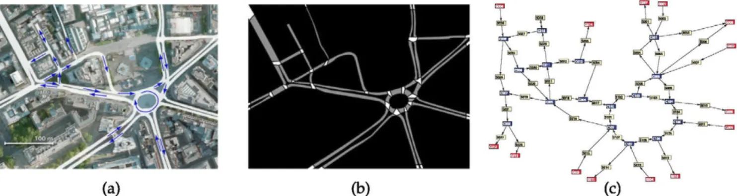
Let the information about the scene be encoded in the input structure M (Fig. 2) reflecting the restrictions imposed by the scene layout on object trajectories. We use a binary mask E>M for the delimitation of passable areas.
The capability to generate plausible p a t h hypotheses requires a mechanism for selecting high-level paths linking two areas of the m a p , namely entry and exit zones. M is therefore defined using a dual representation consisting in the separation of passable regions into different units or nodes. Nodes are of three types: segments (S), crossroads (C), a n d gates (Q). S nodes are portions of the m a p linking two C or Q nodes, C nodes represent regions w h e r e two or more S nodes converge, and Q nodes indicate those regions w h e r e objects can e n t e r / e x i t the scene. Q nodes are distin-guished between entry (appearance) a n d exit (disappear-ance), denoted respectively by QA a n d Qo. We denote by M the whole set of nodes n of the m a p . Using this division of the scene, high-level paths between pairs of regions can be expressed as ordered sequences of nodes.
Additionally, w e consider a connectivity matrix CM indicating the direct vicinity b e t w e e n pairs of nodes in the structure M. This binary matrix expresses implicitly the direction(s) each n o d e of the system can be traversed in. CM is, by construction, sparse: this characteristic allows the use of efficient graph-search algorithms for
(a)
Fig. 2. Description of the map structure M. (a) Environment (Copyright 2012 Google-Map data), (b) Individual binary masks B„ for all the nodes com-posing M (S nodes in grey, C and Q in white), (c) Connectivity graph (S in yellow, C in blue and Q in red).
discovering high-level paths linking two areas of the m a p such as the classical fc-shortest p a t h search algo-rithm by Yen [28] or other equivalents [29].
To include spatial characteristics, each n o d e n has an associated binary mask B„ indicating its extent, a n d such that, ideally, B„ n Bn/ = 0, Vn, rí e M with n ^ n', and BM = UvtieA) ^n- Additionally, each QA n o d e is described as a point b„ 6 IR2 indicating its corresponding expected object entry position.
3.2 Proposed Bayesian Formulation
The inference of E is based on two main sources of informa-tion: the partial locally observed trajectories (Í1,) -ej- a n d the m a p M. Their influence has a considerable associated uncer-tainty, which can be modeled statistically. We analyze the camera positional parameters E and their associated uncer-tainty by expressing the posterior distribution p(E | í l , M) from both sources. However, E a n d the observation i l j of a certain object are not directly related: the observed track il}
will be determined by E a n d by the absolute trajectory R, of the actual underlying object which caused the observation. For this reason, w e introduce explicitly object trajectories R = (Rj)i€j (with Rj as defined in Section 5.1) as auxiliary
variables to indirectly obtain the posterior distribution for E: defining first the posterior joint distribution p(E, R J í l , M), and then marginalizing it over the space of possible object routes to obtain
p ( E | í l , M ) = / " p ( E , R | i l , M ) d R , (2)
where the integral should be considered mere notation. The use of the indirect expression (2) is motivated by the fact that the joint distribution allows a satisfactory decomposi-tion in terms of the two previously discussed sources of information as, via Bayes' rule, w e can write
p(E, R | í l , M) ex p ( i l | E , R , M ) p ( E , R | M ) . (3) The first factor on the right-hand side, the observation or like-lihood model, represents the probability distribution of the 2D tracks Í1 for given E a n d R. The second factor, the prior distribution, encodes the information on the u n k n o w n s before any experimental data have been observed. Their definitions are detailed in Section 5.1.
This indirect definition of the posterior distribution p ( E | í l , M) does not allow an analytic study of its main characteristics. For this reason, w e construct an empirical
=(1A) JJ
distribution from a set of U samples {E }u = 1 d r a w n from it, obtained using Markov chain Monte Carlo (MCMC) methods [30].
Since the observed tracks could be consistent with multi-ple camera positions in the m a p (e.g., straight passable regions that d o not present e n o u g h distinctive features), the estimation of the camera position may present an inherent ambiguity. We detect these ambiguous settings by
=={u) JJ analyzing the sample-based representation {E }u = 1 of p ( E J í l , M). This analysis, performed using an adaptation of the K-adventurers algorithm [31], allows us to infer the set
/¡A
TV-{E }k=i of K < U distinct approximate camera position
hypotheses that best approximates the sampled distribution in terms of the Kullback-Leibler (KL) divergence [32]. This generates an estimate of the relative plausibility of the retained hypotheses that quantifies the ambiguity of the given setting. , .
={u) JJ
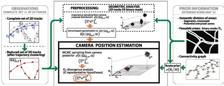
The generation of the samples {E }u = 1 via MCMC requires at each iteration the evaluation of the posterior probability for the p r o p o s e d camera hypothesis. H o w -ever, the marginalization process described in (2) cannot be performed analytically. For this reason w e design a sequential Monte Carlo algorithm b a s e d on importance sampling ( A p p e n d i x A). A l t h o u g h efficient, this process impacts the computational cost of camera hypothesis evaluation. To overcome this p r o b l e m , w e take two addi-tional steps. First, w e simplify the set of available tracks using u n s u p e r v i s e d trajectory clustering [33] that gener-ates a r e d u c e d set of representative tracks. Second, w e define a preprocessing module aimed at g u i d i n g the search within the solution space a n d t h u s compensate for the fact that p(E | í l , M) presents, in general, a considerable n u m b e r of sparsely distributed m o d e s . This m o d u l e esti-mates a p r o p o s a l distribution g(E | í l , M) by checking the purely geometric consistency b e t w e e n observed object positions a n d passable regions of the m a p . The principal mod-ule concerns the MCMC sampling process itself, g u i d e d by this proposal q (E | íl, M), and the Kullback-Leibler diver-gence analysis (Fig. 3).
4 PREPROCESSING: GEOMETRIC ANALYSIS
The aim of the geometric analysis module is the generation of a proposal distribution density g(E | í l , M) (from n o w on, g(E | M)) expressing the plausibility of each camera position according to the purely geometric consistency between the observed 2D tracks a n d the map.
Let us assume a positive function / ( E ; íl, M), evaluable at each E a n d measuring the fit of point-wise observations and binary mask BM, such that g(E | M) ex / ( E ; i l , M ) . We can use a different importance sampling distribution z(E) for extracting samples from to obtain the set {E1-^, w^' }s = 1 of
weighted samples, with &s> ~ z(E) and
These samples are used for approximating the desired den-sity g(E | M) by the kernel-based function
g ( E | M ) = l ^ > ( É M ) f c ( E - É M ): 3=1
w h e r e k (E) is a multidimensional kernel function (integrat-ing one over its whole domain), defined over the continuous space IR2 x SO(2) (therefore, kernel density estimation tech-niques a d a p t e d to this partially cyclic space are used). This approximation is both operational a n d accurate, a n d con-verge as S —* oo to the convolution g(E | M) * &(E) (Appen-dix B). For simplicity, w e use i n d e p e n d e n t kernels for each dimension of E. The kernels of the two spatial dimensions have been chosen Gaussian. The kernel of the angular com-ponent has been considered Gaussian with truncated tails,
OBSERVATIONS COMPLETE SET Q OF2DTRACKS
- Complete set of 2D tracks
- Reduced set of 2D tracks (after trajectory clustering)
PREPROCESSING: GEOMETRIC ANALYSIS (2D tracks VS binary mask) Importance sampling from camera
proposal distribution g(E | ( t l / ^ j , M )
Kernel-based aproximation to q(E | (njLj, M)
? ( E | ( Q ^ , , M )
CAMERA POSITION ESTIMATION MCMC sampling from camera
posterior P( E | ( £ % , , M )
KL-divergence analysis (ÍT representative hypotheses)
({E^C
PRIOR INFORMATION EXTENDED SCENE MAP M Semantic division of areas: ; > - semantic aivision or areas: i ^ ^ " ^ " ™ ^ 'Segments, crossroads i • Potential entry/exit zones
- Passable areas: binary masks!
,
LPS!
Fig. 3. System overview: preprocessing and principal modules, and input and output variables at each stage.
since angular kernel b a n d w i d t h m u s t b e clearly lower than 2JT to avoid affecting excessively the shape of the obtained kernel-based approximation.
We define the importance distribution as
z(E) = z(c,cp) =p(c\M)q((p\c, M) (4)
where p (c | M) represents a certain prior distribution for the camera location aimed at increasing the rate of camera hypotheses generated in the proximity of the passable regions of the m a p (but w i t h n o direct relationship to the cal-culation of the posterior distribution (7)); q(<p | c, M) is expressly chosen so as to coincide w i t h the conditional dis-tribution of (p. The definition of p (c M) is based o n the assumption that cameras are placed in order to monitor moving object behaviors. Thus, assuming that the origin of the camera local coordinate system 3&c is close to the centroid of the transformed FoV onto the g r o u n d plane, locations c that are closer to the passable areas of the m a p should have a higher probability. This is fulfilled b y the distribution
p(c | M) 1 BA c e B M 1 2TZOI !( c
-where B M represents the set of m a p points corresponding to the center positions of the pixels indicated as passable in the binary mask of the scene a n d ac controls the extent a r o u n d BM •
The definition of the importance density (4) simplifies weight calculation into
w(E M g(c r W p(cM | M)
M)
fx/
027r/(£W^;a,M)d^
p(cM | M) (5)
and allows hierarchical sampling for E1-^ b y first extracting cM from p(c | M) a n d using this c ^ to apply integral trans-form sampling [34] o n q(jp c, M). The integral
QO;c
?(*) g ( £ | £W, i l , M ) d £ :jg7(c('),£íi,M)dc;
jf7(ÉM ?;il,M)<
required for transform sampling is obtained using linear interpolation on / ( c ^ , <p; í l , M) (as a function of <p only) by evaluating this function for a relatively low n u m b e r of ori-entations. This approximated integral is also used to set the numerator of (5) for weight calculation.
To illustrate the p r o p o s e d sampling approach, valid for general positive functions / ( E ; í l , M), w e propose the fol-lowing / ( E ; Í1, M) = rY, w h e r e y > l a n d
" ( i l ; E , BM) =
£
j e Jn.
teT(fi,-i_
w h e r e an is the standard deviation of the observation noise (Section 5.1.1) a n d Í¿M(0 is the Euclidean distance to the m a p mask BM- The p r o p o s e d consistency-checking function highlights hypotheses E that are in line w i t h the m a p a n d the observations while avoiding penalizing mismatches d u e to observation noise.
5 CAMERA POSITION ESTIMATION
The camera position estimation m o d u l e analyzes p(E | í l , M), defined as the marginal of the factorized joint distribution. Its main characteristics will b e captured by a set of K weighted camera positions {E , vffl }k = 1
represent-ing hypotheses a n d the inherent ambiguity of the settrepresent-ing.
={u) JJ
For this p u r p o s e , U samples {E }u = 1 are d r a w n from the posterior p(E \ í l , M) by MCMC sampling using the result of the preprocessing m o d u l e as a proposal density. The set
EW
wm\
K{E'
}k=i is estimated b y searching the subset of Ksamples in the generated sample set {E }u = 1 that approxi-mates best the empirical posterior distribution in terms of the Kullback-Leibler divergence.
5.1 Probability Model Definition
Because camera E a n d route parameters R are conditionally i n d e p e n d e n t given the m a p , the joint posterior distribution (3) can b e further factorized:
p(E, R | M) = p(E | M) p(R | M). (6) This factorization allows us to naturally integrate different
sources of information on the absolute camera location, such as GPS, Wi-Fi based analysis [35] or other sensor locali-zation algorithms [12]. W e a s s u m e a non-informative prior for E, discarding from n o w on the term p(E | M) in the expression of the posterior distribution.
We a s s u m e conditional i n d e p e n d e n c e b e t w e e n routes of different objects (Rj)j<£j given M. Additionally,
obser-vations ilj corresponding to different objects can be con-sidered conditionally i n d e p e n d e n t given the true routes Rj that generated t h e m a n d i n d e p e n d e n t from the m a p . This consideration, along w i t h those previously given to (6), allows us to write the joint posterior distribution in (3) in terms of i n d i v i d u a l observation models a n d route priors as
p(E, R | Í1, M) ex Y[{P(il3\E,R,)P(R3\M)}. (7)
The specific definitions proposed for the two individual probability distributions retained in (7) involve the auxiliary variables Rj representing real object trajectories d u r i n g their presence in the scene. Their definition has been chosen to reflect the environmental influence on objects: they "decide" which high-level p a t h to follow across the scene (i.e., entry and exit regions) a n d the sequence of regions followed to link them. Moreover, they move locally so as not to violate the positional a n d dynamical restrictions imposed by its previous high-level choice. These considerations leads to a two-level representation
which explicitly contains the high-level p a t h Tij followed by the object across the m a p as well as the low-level descrip-tion (T(Rj), (r*, v'-)teT/R.N) of the route itself. The usefulness of this definition is clarified in Section 5.1.2.
Tij is defined as a sequence of high-level nodes of the m a p M expressing the areas to be traversed to link an entry and exit node. As for the low-level description of the route, the m o v e m e n t of the objects, of continuous nature, is mod-eled as a discrete process with the same framerate of the observed 2D tracks i l j . T(Rj) indicates the interval of conse-cutive time steps d u r i n g which the considered object is present in the scene (which is, in principle, u n k n o w n ) , and the time-stamped pairs (r*, v') represent the position and velocity of the object at time t expressed with respect to the absolute frame 3&TO. Although neither Tij nor v* are directly observable, they are included in this definition to ease object dynamics modeling.
5.1.1 Observation Model
Our definition for the observation model p ( i l j | E , Rj) of each individual object is inspired by [12] a n d considers only positive observations (i.e., the lack of observation is not modeled). Although w e write p ( i l j | E , Rj) for clarity, the
1. As made clear from the observation model defined in Sec-tion 5.1.1, multiples of this framerate could be used without major modifications.
observation process is the noisy registration of the true posi-tions of the j t h object over time. Thus, it w o u l d be more appropriate to explicitly indicate that neither the high-level p a t h Tij followed by the object nor its velocity are actually involved. So,
p(% | ER,) = p(K-)
teT(ilj)| E ^ R , ) , (rJ)
teT(Rj)).
We a s s u m e that all possible observation time spans T(ilj) such that T(ílj) C T(Rj) are equally probable, a n d that point observations corresponding to time steps out-side the route time s p a n T(Rj) are impossible. The former a s s u m p t i o n h a s no effect on the practical use of piflj | E, Rj), since it is u s e d in practice as a function of E a n d Rj w i t h T(tlj) fixed a n d k n o w n . Both, along w i t h the a s s u m p t i o n that the observations <w* at different time steps are conditionally i n d e p e n d e n t given Rj a n d d e p e n d only on the true position r* of the object at its correspond-ing t, lead to
f J ] K4l
E>
r5)> T(n
3)CT(R
3)
:p(Q,j\E,Rj) oc I teT(fij)
{ 0, T ( % ) g T(R3):
w h e r e the contribution p(&>'|E, r ' ) represents the specific observation process at time t.
As for the observation, w e assume that each point &>' is the true position of the corresponding object route Rj with respect to the local (metrically-rectified) ground-plane coor-dinate system 3&c associated to the camera plus an additive, normal, homogeneous and isotropic noise. In these condi-tions w e can write
p ^ - l E r ^ G ^ ^ S f i ) , (8) which represents the probability density function (pdf) of
the n o r m a l distribution TV'tó; v', Xf»). The covariance matrix Sfi = Ofi E assumed constant a n d isotropic for convenience [36], represents the zero-mean observation noise a d d e d to v', which represents the route position r* expressed in the local coordinate system 3&c as
v\ = m1 (rj; c, <p) = ( R O P ) )- 1 (V) - c),
w h e r e m_ 1(-;c,(p) is the inverse of the linear isometry (1). However, the density p (&>' | E, r ' ) is used in (7) as a function of the absolute object position r ' , with oÁ assumed fixed. Using the isotropy of the considered distribution a n d the isometry m(-; c, <p) w e can rewrite
p ( m E , r J ) ^ G ^ v ^ S n ) ,
w h e r e v* = m(<w';c,<p). We use this equivalent reinterpreta-tion, a n d not (8).
5.1.2 Route Prior Model
The use of specific information on the scene allows a realis-tic modeling of object dynamics. The aim of the route prior model is to interpret the characteristics of the m a p M and translate them into a set of statistical relationships
controlling the m o v e m e n t of objects. O u r p r o p o s e d model is divided into two factors concerning, respectively, high-level and low-level features as
p(R3\M) = P(H3\M)p(T(R3 írÉ vtN| H„M). (9) The first factor, the probability of a certain high-level p a t h Tij, allows probability definitions based on criteria such as distance, sharpness of turns or privileged areas. W e define a prior for Tij that first selects one entry a n d one exit n o d e for the route from, respectively, QA a n d Qo, with uniform prob-ability as in principle n o information on the origin a n d des-tiny of objects will be available, a n d penalizes longer paths between the t w o selected Q nodes. Using the representation Tij = (riA,Ti°,vi£i) with Ti° representing all the intermediate nodes of the path, this can be written as
P(Hj | M) = P(nA | M) P(nD | M) P{H° \ nA, nD, M),
where the two first factors are uniform a n d thus constant for all objects, whereas the latter has been chosen to b e propor-tional to the inverse of a p o w e r of the length l(Tij) of the complete path, penalizing longer p a t h s as:
P(m\nA,nD,M)0c(l(nj)y a > 1.
The latter term of t h e factorization (9) models all the low-level aspects of the route Rj (given Tij), n a m e l y its time s p a n T(Rj) = (t®,..., t?) a n d t h e position r* a n d velocity v* of t h e object at each time step in T(Rj). As for tQ-, representing the time w h e n the object first enters
the scene, w e consider a non-informative (uniform) prior defined o n a time range, equal for all t h e NQ objects in the scene, long e n o u g h to guarantee that all routes con-sistent w i t h the tracks i l j are included.
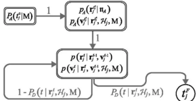
We assume that low-level routes of objects can be mod-eled as a first-order Markov process. This assumption allows the simulation of low-level routes in a simple a n d fast manner, essential for route marginalization (Appendix A). Moreover, it prevents an artificial explicit modeling of the duration of T(Rj) since route length can b e implicitly considered in the p r o p e r Markov model b y including, at each time step, a certain disappearance probability PDU I r'., Tij, M). This probability d e p e n d s on the distance from the position r* of the object at each time step to the spa-tial s u p p o r t Bnp of the exit n o d e tip of the high-level p a t h Tij. This Markov model, depicted graphically in Fig. 4, results in
pin*,,),^) \H„M)
PAWWPA ( r / , v HhM I I [ i1 - po(* I 4 Hi, M))p(r5+\ v5+1 |rj, vj, H3, M) Pi,(if | r / ^ M ) , (10) PAQ°\M)TT
pVAtw)
p(y'\r',vj',7fj,M)f
p,(t\^,»„ti) (if
Fig. 4. Prior low-level route distribution, defined as a Markov process.
w h e r e w e have explicitly indicated that the first time step of the route follows a different model, denoted by PA{) from the rest of T(Rj). The disappearance probability term PD (t | r ' , Tij, M) is a binary function such that objects always continue their w a y whenever r* has n o t reached ~BnD (which
is equivalent to disappearance probability identically zero) and always disappear immediately w h e n they reach Bni3 (disappearance probability identically one).
As for the Markovian term for position a n d velocity time evolution, w e use the decomposition
p^vJIrfSvfST^M)
V r , r ' - S v ^ V v4 3 i V J r - v
.rí-ST^M),
which allows the i n d e p e n d e n t definition of position a n d velocity evolution models (dependencies are explicitly indi-cated). The first term is the distribution of the position r ' and reflects the assumption that the velocity v '_ 1 at time t — 1 w a s chosen so as to cause a reasonable object location at t, a n d that n o major deviations from the resulting linear evolution are experienced. For this reason, w e setptti-r
1.^
1)
G ( r ' . ; i , ' Xr (11)w h e r e Sr = a^ I represents the covariance matrix of the iso-tropic zero-mean normal prediction noise a d d e d to the expected position rf- = r '_ 1 + v'-_1.
As said above, v. is chosen so as to generate a satisfactory position r '+ 1: thus, p(v'-1 r'-, v'~1,r'~1,?i7-,M) is responsible for reflecting the main characteristics of the trajectories of the specific moving objects. For this reason, it should b e defined taking into account the specific environment (indoor/out-door, urban) a n d moving object type (vehicles, pedestrians). To illustrate the creation of p(v* | r ' , v'-_1, r^_1, Tij, M), w e use here an u r b a n traffic model. However, other types of envi-ronments a n d moving objects w o u l d b e equally compatible with the presented framework.
Our definitions for u r b a n traffic dynamics stem from the following assumptions: (i) local behavior of vehicles with respect to t h e local characteristics of their trajectories varies slowly; (ii) vehicles tend to m o v e along the tangen-tial direction of their high-level p a t h Tij a n d to a certain average speed VAVG w h i c h d e p e n d s o n t h e scene itself; a n d (iii) vehicles keep their position w i t h i n the passable regions composing t h e high-level p a t h Tij, t e n d i n g to leave a certain distance W b e t w e e n their expected
position rt+l a n d t h e limit of Tij. W e u s e t w o auxiliary
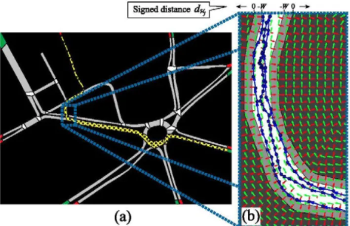
structures to define a practical p(v'-1 r'-, v'~1,r'~1,?i7-,M) fulfilling these properties: the signed Euclidean distance d-H. (r) to t h e limit of the binary mask B-«. of Tij (with neg-ative values inside Tij passable regions, a n d positive out-side) a n d the unitary tangential vector field T-^.(r), orientated t o w a r d s the direction of vehicles along the p a t h Tij. The former is u s e d for influencing or "correcting" vehicle positions near the limits of the u n d e r l y i n g high-level path. The latter allows t h e defini-tion of a " m o v i n g " local coordinate system indicating, at each point, t h e tangent a n d n o r m a l directions of the given p a t h , m a k i n g t h u s possible to p r o p a g a t e t h e local behav-ior of objects along their trajectory. Both d-n,(r) a n d rft.(r), a n d all t h e structures derived from them, will be calculated o n a discrete spatial grid t h r o u g h simple oper-ations performed o n t h e binary m a s k B-« a n d evaluated later o n a n y continuous position using interpolation. Using these structures, w e define
P{
4-
1 ,t-i ,Hj,M)G(v5-;/4£
vwhere Sv = o\ I is the covariance matrix of the isotropic zero-mean n o r m a l prediction noise a d d e d to a n expected velocity defined as the s u m /x* = v + vc( r ' , v ), where v represents the adaptation of the velocity v '_ 1 of the object at r '_ 1 to the local characteristics of its p a t h at r ' , a n d where vc represents a correction function aimed at keeping object position within the path.
As for the a d a p t e d velocity term v , w e assume that the tangent a n d n o r m a l components of v '_ 1 are kept a n d adapted individually as
xn, r L
) K
where n-n (r) represents the n o r m a l vector that forms, along with fft.(r), a positive reference system at r. To encourage routes with tangential speed close to VÁvG/ the function gT(-)
controlling the scalar evolution of the tangential velocity component is defined as
9r(V) = giV + g0, with
0 < g0 < VAVG.
9i = 1 - 9O/VAVG-,
contractive with fixed point at VAVG- Analogously, to encourage objects to move exclusively along tangential tra-jectories, the function gn{) controlling the scalar evolution
of the n o r m a l component is defined contractive a n d anti-symmetric (thus with fixed point at the origin) according to
gn(V) = g2V, 0 < g2 < 1.
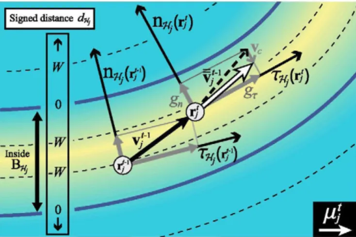
Fig. 5. Schematic description of the velocity evolution of objects: compu-tation of i^.. Background gradual colouring indicates dnj(r), from yellow
(negative) to blue (positive).
than — W for a certain positive W. O u r p r o p o s e d correc-tion factor is of the form vc( r ' , v- ) = wc(r', v- ) Vd-w.(r) for a certain scalar function vc(-), w h o s e definition stems
from t h e a p p r o x i m a t i o n
«M'i + vT+v,
<M
rJ.
= t - i
+ v.
VdHj(v)+vc,w h e r e w e have used that ||Vd-H || = 1 for the Euclidean n o r m in the regions of interest (note that it represents the spatial rate of change of the spatial distance). The scalar cor-rection function vc(d) is then defined as
vc(d) = 0;
-(d + Wexp{-(l + d/W)}):
d<(-W), d>(-W),
which satisfies the above requirements a n d which obviously reduces the distance of all object positions such that —W < dff. < 00. The velocity evolutionary model for vehicles is illustrated in Fig. 5.
The prior distribution for the position and velocity of the vehicles at their initial time step t°- is defined as
PA r / , v / |W,-,M =PAM \nA) PAM \rLUuM
Both initial position a n d velocity are considered isotropic and normally distributed, a n d centered respectively at the expected entry point hnA of the entry n o d e VIA a n d the
t° t° e x p e c t e d t a n g e n t i a l v e l o c i t y ¡i • = VAVG TTÍ, (r/ ) •
Fig. 6 displays different routes simulated using the pro-posed dynamic model for a certain high-level p a t h Tij, showing that our proposal is able to capture the restrictions imposed b y the environment.
The distance correction term vc( r ' , v ) aims to com-pensate the expected position (r* + v ) so as to keep the resulting distance d-u to the b o r d e r of t h e p a t h below zero (i.e., inside its m a s k B-«.), leaving velocity unaltered w h e n t h e expected position h a s signed distance lower
5.2 Numerical Evaluation of the Posterior
The posterior pdf p(E | Í1, M) is defined as the marginaliza-tion of p(E, R J í l , M), factorized as (7), over R. This process can b e divided into t w o steps: first, marginalization of p ( E , R | i l , M ) over the low-level details of all R,- (j e J), which can be written as
Signed distance i/« r-—"" ^ . .
u ..•*,'H
Fig. 6. Example of route simulation with the proposed dynamic model, (a) First, high-level path 7i, sampling (dotted), (b) Low-level route gener-ation using the fields zH.(v) and VdH. (green and red) and partial magni-fication of three simulated routes.
p(E(^),
e,l(^W>
•Vjej- M)
=n
E
p ( i l , - | E , R; /) p ( R , - | M ) d ( r ' v vr(Ri)-'(r*.vpteT(Ri; p j/teT(Rj]E / P^-I^R^P^-IM)
Vr(Ri)-'(r*.vpteT(Ri)P W , ( 4 V ; )
J ' j/teT(Rj]H
3MW^))
p j/teT(Rj]= J ] !
p(
wí I
M) ME, «,-;%)] =
where d(r', v'-)ier(R:, indicates that integration is carried out over all positions a n d velocities in T(Rj) and with
h(E,H
j;Cl
j)= J2 [ P(%|E,R,-)
Vr(Ri)"'(r*.vpteT(Ri)(13)
and second, marginalization of (12) over the discrete sub-space of possible high-level routes across the m a p to isolate completely the camera position E, obtaining
(14)
p(E | (íl,-)
ÍGi7, M) = J2 P(
E- (
w¿ W I (% W >
M)
V{(Wj)jej}
^IIE^^IM)^,^^,)].
The evaluation of p (E | í l , M) is based on the estimation of the s u m / i n t e g r a l unit h(E,TÍJ;Ü,J) for each high-level p a t h Tij of each object. The MCMC sampling process from p (E | í l , M) (Section 5.3) requires the frequent evaluation of (14): for this reason, w e have designed an efficient algorithm for estimat-ing h(E,Tíj;ü,j), based on sequential Monte Carlo methods and importance sampling as detailed in A p p e n d i x A.We also apply high-level p a t h grouping to improve the efficiency of the marginalization process. This simplification is rooted in the fact that the calculation of h(E,Tíj;ü,j)
Fig. 7. High-level path grouping performed at the principal module. Three paths enclosing the true absolute 2D track and thus sharing the same central nodes (depicted as low-level routes). Unlike path 3, paths 1 and 2 belong to the same class (same nodes around the track).
involves only the observations &>', expressed as m(&>';E) with respect to the absolute frame of reference 3R„ (where m(-;E) is the isometry (1)): thus, high-level p a t h s differing only in aspects that do not affect the low-level route distri-bution in the areas a r o u n d m(&>';E) m u s t provide similar h(E,Tíj;ü,j). Low-level dynamics defined in Section 5.1.2 are determined by the fields d-uAv) a n d T-W. (r), calculated using local characteristics of the mask B-« of the high-level p a t h TLf. therefore, all paths Tij having an identical B-« "before" (according to the direction of Tij) and in the area w h e r e the observations m(<w'.;E) lie m u s t yield the same (12) ^(E, Tij; Clj). For this reason, all those Tij w h o s e nodes
coin-cide until the position of the last of the point observations m(<w'-;E) are grouped, a n d h(E,TÍJ;Ü,J) is only evaluated once for them all.
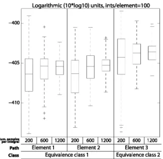
Additionally, although it is not exact, w e can follow a similar reasoning for those nodes composing the high-level p a t h Tij "before" the observations m(&>';E), t € T(flj), and assume that the distribution of route low-level characteris-tics "forgets" its details after a certain distance. We perform thus a previous analysis for grouping high-level paths into a reduced set of classes, characterized by sharing the same preceding A^pre a n d posterior A^post nodes a r o u n d the obser-vations of the corresponding object. Integral calculations are then performed only for one representative of each class. This simplification (Fig. 7) reduces drastically the n u m b e r of integrals and therefore the computational cost associated to the evaluation of p(E | í l , M). Fig. 8 shows that the differ-ences between the integrals of different elements belonging to the same class (A^pre = iVpost = 2) are m u c h lower than the variance of the integration algorithm itself, which justifies the grouping process.
5.3 MCMC Sampling and Move Definition
The proposed sampling process based on the Metropolis-Hastings algorithm [37] considers two moves: m o v e 1 (mi), the modification of a previously accepted camera hypothe-sis; a n d move 2 (m2), the proposal of a n e w camera hypothe-sis from the data-driven proposal g(E | M) estimated in the preprocessing module, n e e d e d to reach distant regions of
-400 -405 -410 Num.umpl« per integral Path Class
Logarithmic (10*loq10) units, ints/element=100
200 600 1200 Element 1 200 600 1200 Element 2 Equivalence class 1 200 600 1200 Element 3 Equivalence class 2 Fig. 8. Evaluation of the integral h(E,Hj-,ilj) for the three paths in Fig. 7 (100 different runs per path and number of samples, probability expressed in logarithmic units). Relevant statistical indicators showed as a box plot.
the solution subspace. The moves will be chosen w i t h proba-bility q(mi) a n d g(m2), respectively, with q(mi)+ 9(7712) =
1-Move 1 uses a proposal kernel g(E | É) normal a n d cen-tered at the previously accepted sample E to d r a w a n e w hypothesis E. Thus, g(É | É) = g(É | É ) , and the resulting acceptance ratio for a n e w hypothesis E is a\ = min{l,cii}, where
» i
7 j ( E | í l , M ) g ( m i ) g ( É | E ) ' p ( É | í l , M )g( m i ) g ( É | É )
n
í Gy [ E v H ; . ^ I M ) M É , «;•;%)
(15)a n d w h e r e h(E, TLf,ííj) represents the low-level route integration unit discussed in A p p e n d i x A. In m o v e 2, w h e r e the generation of n e w hypotheses E is directed by the kernel-based p r o p o s a l g(E|M), acceptance will be driven by the ratio a2 = min{l,ci2}, w h e r e
a2 p ( É | í l , M ) g ( m2) g ( É | M ) 'P(É\Q,,M)q(m2) g ( É | M ) « i
-g(É I M)
g(É I M)
where, unlike (15), proposal densities d o not cancel mutu-ally a n d m u s t thus be explicitly calculated.
Accepted sample rate strongly d e p e n d s on h o w well the seeds generated in the p u r e l y geometric analysis of the preprocessing m o d u l e fit the d y n a m i c s of the scene, since certain observations can geometrically fit certain areas of the m a p b u t h a v e negligible probability once object d y n a m i c s are considered. To p r e v e n t the unneces-sary evaluation of clearly erroneous camera hypotheses, w e eliminate every checked p r o p o s a l seed that has p r o v e d against the d y n a m i c s of the m a p . This simple action eliminates m o s t erroneous seeds d u r i n g
the b u r n - i n p h a s e of M C M C , a n d improves the accep-tance rate of s u b s e q u e n t iterations.
5.4 Hypothesis Selection and Ambiguity Analysis
The marginal posterior p(E | í l , M) is composed of an inde-terminate high n u m b e r of probability modes sparsely dis-tributed over the solution space. W e summarize the main characteristics of this distribution, that is, its main modes and their relative importance, in a reduced set of distinct weighed camera hypotheses {E , w1-^ }k = 1 using anadapta-tion of the K-adventurers algorithm [31] for multiple hypothesis preservation. For the sake of readability, w e will denote p(E | í l , M) by p(E).
Let p(E) be a certain target pdf, and let
p ( E ) = £ « j W G ( E - E ' •WN (16)
be a kernel-based approximation with exactly K modes, w h e r e G(E) represents a kernel profile centered at the origin and with fixed scale (adapted to the expected size of the searched modes). We aim to find the set {E , w ^ }k = 1 of
weighted solutions that best approximates p(E) in terms of the Kullback-Leibler divergence
DKL(P\\P] p(E) In P(E)
p(E) dE -H(p) + H(p,p), w h e r e H(p) a n d H(p,p) are, respectively, the entropy of p(E) and the cross entropy of p(E) a n d p(E). Since H(p) is constant for all possible solution sets, this problem is equiv-alent to the minimization of
H{p,p) = - Ep ( E )< ! l i
£ V * ) G ( E - E
{k)\ k=\w h e r e EP( E ) [ • ] is the expected value w i t h respect to the ref-erence probability density function p(E). H(p,p) can be inferred using the RMSE estimator for the m e a n as
H(p,p)
U
E
1
» E
^ ) G Í I
W- E
( t ) (17)w h e r e E ~ p(E). In our case, the U samples are the result of the MCMC step discussed in Section 5.3.
The best s u m m a r i z i n g set {E ,W'k'}k=1 is searched
amongst the samples {E }u = 1. Subsets of K samples are r a n d o m l y chosen a n d analyzed, a n d the best in terms of H(p,p), along w i t h its corresponding weights {w^'}k=1, is
finally retained. The weights {w^'}k=1 for each test set (k\
TV-{E }k=i are suboptimally estimated using Lagrange
opti-mization on a conveniently simplified version of (17), w h i c h stems from the a s s u m p t i o n that the K m o d e s are separated e n o u g h w i t h respect to the scale of the kernels G(E). In these conditions, the area w h e r e p(E) is signifi-cant can be fragmented into subregions {¿-W}f=1 w h e r e E 6 Z1- ^ a n d the contribution of the corresponding
(k\
Fig. 9. Synthetic database: object routes (blue), fields of view of the cam-eras (red).
(16) for p(E) can be a p p r o x i m a t e d by
p(E) = f > « G ( E - E
(V ^ ) ( E ) L
fc=iwhere Iz(k) (•) is the indicator function. This region-based
approximation allows us to write the logarithm of the s u m as a s u m of region-related logarithms, which transforms (17) into
H(p,p) U = l 1 u K (
J2^G(^
U)-E
(y
z{jE
iu] U u=l k=\5 « G [ E
# ) IZ(K) ( E (18)This last expression is suitable for the method of Lagrange multipliers, applied to find the set {w^}k=1 that minimize
H{p,p) subject to the restriction ^2k=1 w1- •> = 1 (note that the
additional restriction w1- •> > 0 is in principle required, b u t
has no effect in this case as s h o w n by the result). The con-struction of the Lagrange function
A(w,A) = ff(p,p) + A(2>(
f c)-l
and the resolution of its resulting system of equations VA(w, A) = 0 yield the final weights
^
}
4&
zWU<
,Vke{i,...,K}.Although the preceding formulae are totally general, we assume a kernel profile G(E) composed of independent Gaussian (pseudo-Gaussian in the angular component) functions for each dimension of the solution space.
The inference of the n u m b e r K of significantly distinct modes is important itself to u n d e r s t a n d the ambiguity of the given setting. O u r proposal for its automatical inference
W
-Jfev J mlMZZ
I i
b)
Fig. 10. Real vehicle data set, camera 1: a) View, b) Local ground-plane frame of reference, once camera-to-ground homography has been applied. Black lines: 2D tracks for all objects included in the data set. Red lines: the eight representative tracks retained after trajectory clus-tering [33].
iteratively increases in one unit the n u m b e r K of assumed modes, w h o s e corresponding (sub)optimal KL-divergence is estimated a n d compared to the best divergence with K — 1 modes. The algorithm ends w h e n the gain obtained by a d d i n g a n e w m o d e is below a certain percentage of the best divergence hitherto.
6 EXPERIMENTAL VALIDATION
6.1 Experimental Setup
The p r o p o s e d framework a n d the d y n a m i c m o d e l dis-cussed in Section 5.1.2 are tested using b o t h synthetic data a n d a real database. All the results h a v e b e e n gen-erated using go = VAVG/20 a n d g2 = 3/4 in the dynamic
m o d e l definition (values w i t h i n a reasonable range a r o u n d these s h o w n o major deviations), a n d a low n u m b e r of orientations ( « 4 0 ) for integral evaluation in the preprocessing m o d u l e .
The synthetic database consists of a real road scene for m a p definition and semi-automatically generated trajecto-ries. The m a p covers an u r b a n extent of 500 x 400 m, a n d its associated binary masks have a resolution of 0.33 m / p i x e l (Fig. 9). Object average speed w a s 35 k m / h , test routes were generated at a framerate of 5 fps, a n d the FoV covered by the camera is rectangular (equivalent to a vertically-oriented camera) a n d of size 50 x 35 m. Ten different cameras have been randomly generated for testing, each one w i t h a n u m -ber of observed 2D tracks between 4 and 10.
The real vehicle database comprises four traffic cameras (referred to as MIT-1 to MIT-4) imaging entries to a n d exits from parking lots. MIT-1 a n d its associated tracks have been adapted from the MIT Traffic Data Set [38], while MIT-2, 3 and 4 are from the MIT Trajectory Data Set [39]. The camera views are related to the scene g r o u n d plane using a metric rectification h o m o g r a p h y calculated manually using the DLT algorithm [40], a n d the resulting "corrected" views are considered the local frame of reference of each camera (Fig. 10). The m a p covers 1,200 x 850 m, a n d its associated masks have a resolution of 0.4 m / p i x e l . Object average speed is 35 k m / h , a n d the framerate of the observed 2D tracks is 4.83 fps (1/6 of the original framerate of MIT-1, 29 fps). MIT-1 contains 93 real vehicle trajectories, b u t only eight different representative tracks were retained after the trajectory clustering procedure [33] (Fig. 10). MIT-2, 3 and 4
V ' ¿op £¡4'
5
Ro.OjM ko.02 ¡0.01; í^atM^j RÍO-OÍ*, • •i\
b.oi, _ ] &^J
<Tfi = 0 m (0 pixels)
o-n = 0.25 m (0.0825 pixels)
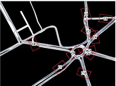
0.5 m (0.165 pixels)
Fig. 11. Camera position hypotheses (green) sampled from the proposal distribution g(E | (il3) e J, M ) estimated at the preprocessing module
for camera C I . Input data contaminated with observational noise of increasing power, and similar obtained results. True camera location (red) and KL-representatives (blue) have been included for clarity.
Sk\\
m.
\ \
^^^gt^M
^ B * A>ai22>
;.#
[
l=_
^ 5
A K B ^o.oeaL_
115
_ /iief ¡CVÍÚI* 5 ^ Ü ^ ^ ^ ^ ^É M
BB^KB
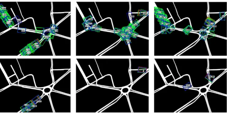
Fig. 12. Preprocessing module proposals (first row) versus principal module results (second row). In green, camera samples generated in each case. True camera location (red) and KL-representatives (blue), with relative weights superimposed, have been included to indicate the estimated uncertainty.
contain, respectively, 4,025, 4,096 and 5,753 tracks, approxi-mately half of them corresponding to pedestrians: after the clustering procedure, 7, 10 and 9 representative vehicle tracks were retained for each camera.
Additional details on the real vehicle databases, espe-cially on the characteristics of the considered camera views and on the u r b a n structures observed from them, can be found in our website.2 The site contains also more detailed descriptions for the synthetic settings, which helps to better u n d e r s t a n d the results discussed in the next section.
6.2 Performance Evaluation
First, w e evaluate the preprocessing m o d u l e a n d the result-ing camera position proposal g ( E | í l , M). Fig. 11 presents results corresponding to the same camera setting b u t with 2D tracks contaminated with different observational noise power. All cases calculate the proposal using 1,000 seeds,
2. http://www.gti.ssr.upm.es/data/CamLocalizationMaps.
and display 100 randomly-generated camera hypotheses showing that the proposals are resilient to noise. Note that the true camera location is included between those that can be p r o p o s e d by q (E | í l , M).
The validity of the integration process used extensively in the principal m o d u l e and based on high-level class grouping a n d iterative MCMC evaluation has been demon-strated in Section 5.3. The K-Adventurer-based analysis has been tested individually, and the corresponding experi-ments have s h o w n that thresholds between 5 and 10 per-cent provide satisfactory estimates for K in most situations. Presented results have been obtained using 5 percent.
As for the overall performance of the principal module, three illustrative results of its effect are included in Fig. 12 showing the difference between the samples proposed before a n d after object dynamics consideration. In all cases, the length of the burn-in phase of the MCMC process have been chosen comparable to the n u m b e r of seeds used by the proposal g(E | í l , M) to eliminate as m a n y w r o n g seeds as possible before the p r o p e r MCMC sampling. We
TABLE 1
Absolute Error of Camera Estimations Performed at the Principal Module versus Baseline Method (*: Straight Zone, Linear Drift, **: Ambiguous Setting)
Cam * C 1 C2 C3 **C4 C5 C6 C7 * C 8 C9 **C10 MTT-1 MTT-2 MTT-3 MIT-4
Proposed approach (principal module) Ambiguity detected YES n o n o YES n o n o n o YES n o YES n o n o n o n o Distance error (m) 58.338 0.731 0.641 134.088 3.214 1.345 1.889 43.606 2.176 182.834 1.129 1.256 0.933 0.786 Angular error (rad) 0.0363 0.0091 0.0107 2.2169 0.0331 0.0120 0.0359 0.0147 0.0091 3.0062 0.0095 0.0163 0.0204 0.0067 Baseline method | Distance error (m) 77.229 297.029 348.045 322.226 304.434 2.119 0.251 87.896 0.219 340.852 1.443 1.615 0.537 1.027 Angular error (rad) 0.0421 0.5608 0.6789 1.2961 0.2474 0.0074 0.0216 0.9149 0.0033 0.1669 0.0225 0.0209 0.0131 0.0114
observe that distributions before a n d after present lower differences w h e n the camera and the observed 2D tracks correspond to an area w i t h especially peculiar geometric characteristics, b u t that the inclusion of object dynamics helps to correctly locate the camera in all cases. The pro-posed K-adventurers analysis has been performed on both estimated g ( E | í l , M) a n d p ( E | í l , M), and its conclusions (representative modes a n d their relative scores) have been included in the figure so as to indicate the ambiguity of each compared distribution.
As for the quantitative performance, Table 1 shows the absolute difference, in terms of b o t h distance a n d ori-entation, b e t w e e n the real camera location a n d the esti-mation performed at the principal m o d u l e , which corresponds to the best m o d e of the K-Adventurers anal-ysis of the data. D u e to the lack of comparable w o r k s in the literature, the table compares the obtained results w i t h a baseline estimation m e t h o d b a s e d on p u r e l y geo-metric point-wise consistency analysis a n d exhaustive search: a grid of 250 x 250 displacements a n d 720 camera orientations (i.e., resolution of 0.5 degrees) is checked, a n d each studied camera position is assigned a score consisting in the s u m of the exponential of the signed Euclidean distances, n o r m a l i z e d by W (Section 5.1.2), of all the corrected 2D points composing the track set Í1.
Table 1 presents results for the cameras of the synthetic and real databases, a n d not only indicates the accuracy reached by our proposal b u t also its ability to distinguish ambiguous settings a n d therefore detecting w h e n the estima-tion should not be considered representative. In the tests, set-tings have been considered " u n a m b i g u o u s " wh e n e v e r the weight associated to the best m o d e is above 0.9. The table shows that our proposal selected a w r o n g m o d e of the poste-rior distribution in two of the 14 tests: this is the case of cam-eras C4 a n d C10, corresponding to settings that fit several zones of the m a p . In other two tests, the correct m o d e was chosen b u t the provided estimate is clearly displaced from the actual location: this is the case of C I and C8, correspond-ing to long straight areas of the m a p resultcorrespond-ing in greatly dis-persed modes. These two inherent ambiguous cases (four tests) are correctly detected by our approach as problematic.
The rest of cameras correspond to less a m b i g u o u s areas that h a v e b e e n correctly identified. In all these cameras, the distance b e t w e e n the estimation a n d the original camera is below 3.3 meters, a n d the orientation divergence is below 2 degrees. O u r a p p r o a c h clearly out-performs the included baseline m e t h o d in terms of reli-ability, p r o v i d i n g satisfactory estimations in all cases. H o w e v e r , the baseline can p r o v i d e slightly m o r e accu-rate estimates in settings such as C7, C9 a n d MIT-3, w h e r e the observed tracks d e t e r m i n e univocally the posi-tion of the camera w i t h o u t considering object dynamics.
7 CONCLUSIONS AND FUTURE W O R K
We p r o p o s e d a framework for automatically estimating the location and orientation of a camera from observed tracks in its field of view. W e use the information of the monitored scene in the form of a m a p that, to the best of our knowl-edge, has not been used before in this type of scenarios, and the adaptation of this information into a probabilistic dynamic model for objects to infer the location a n d orienta-tion of the camera from observed trajectories. Experimental results show the capability of the proposal to analyze differ-ent camera settings, detecting those ambiguous situations w h e r e point estimation is not meaningful, providing satis-factory estimates in rest of cases.
Future w o r k will aim at improving the accuracy of the resulting estimations for the u n a m b i g u o u s settings for example by using low-level details of object routes for opti-mization [41], [42]. Additionally, joint consistency between views could be exploited to disambiguate settings where individual cameras fit multiple m a p areas.
APPENDICES
Appendix A a n d A p p e n d i x B, available as online supple-mental material, can be found on the Computer society Dig-ital Library at http://doi.ieeecomputersociety.org/10.1109/
TPAMI.2013.243.
ACKNOWLEDGMENTS
This w o r k was partially s u p p o r t e d by the Ministerio de Economía y Competitividad of the Spanish Government u n d e r project TEC2010-20412 (Enhanced 3DTV) a n d by the Artemis JU a n d UK Technology Strategy Board as p a r t of the Cognitive & Perceptive Cameras (COPCAMS) project u n d e r GA n u m b e r 332913. Also, Raúl M o h e d a n o wishes to thank the C o m u n i d a d d e Madrid for a personal research grant, which allowed him to do several parts of this work while visiting Queen Mary University of London.
REFERENCES
[1] J. Deutscher, M. Isard, and J. MacCormick, "Automatic Camera Calibration from a Single Manhattan Image," Proc. Seventh Euro-pean Conf. Computer Vision (ECCV), pp. 175-205, 2002. [2] P. Denis, J. Elder, and F. Estrada, "Efficient Edge-Based Methods
for Estimating Manhattan Frames in Urban Imagery," Proc. 10th European Conf. Computer Vision (ECCV), vol. 2, pp. 197-210, 2008. [3] R.B. Fisher, "Self-Organization of Randomly Placed Sensors,"
Proc. Seventh European Conf. Computer Vision (ECCV), pp. 146-160, 2002.
[4] l.N. Junejo, X. Cao, and H. Foroosh, "Autoconfiguration of a Dynamic Nonoverlapping Camera Network," IEEE Trans.
Sys-tems, Man, and Cybernetics, vol. 37, no. 4, pp. 803-816, Aug. 2007.
[5] O. Javed, Z. Rasheed, O. Alatas, and M. Shah, "KNIGHT: A Real Time Surveillance System for Multiple and Non-Overlapping Cameras," Proc. IEEE Int'l Conf. Multimedia and Expo (ICME), vol. 1, pp. 649-652,2003.
[6] N. Krahnstoever and P.R.S. Mendonca, "Autocalibration from Tracks of Walking People," Proc. British Machine Vision Conf., vol. 2, p. 107, 2006.
[7] B. Micusik, "Relative Pose Problem for Non-Overlapping Surveil-lance Cameras with Known Gravity Vector," Proc. IEEE Conf.
Computer Vision and Pattern Recognition (CVPR), p p . 3105-3112,
2011.
[8] M.B. Rudoy and C.E. Rohrs, "Enhanced Simultaneous Camera Calibration and Path Estimation," Proc. 40th Asilomar Conf. Signals,
Systems and Computers (ACSSC), pp. 513-520, 2006.
[9] Y. Caspi and M. Irani, "Aligning Non-Overlapping Sequences,"
Int'l ]. Computer Vision, vol. 48, no. 1, pp. 39-51, 2002.
[10] M. Noguchi and T. Kato, "Geometric and Timing Calibration for Unsynchronized Cameras Using Trajectories of a Moving Marker," Proc. Eighth IEEE Workshop Applications of Computer
Vision, p. 20, 2007.
[11] N. Anjum and A. Cavallaro, "Automated Localization of a Cam-era Network," IEEE Intelligent Systems, vol. 27, no. 5, p p . 10-18, Sept/Oct. 2012.
[12] A. Rahimi, B. Dunagan, and T. Darrell, "Simultaneous Calibration and Tracking with a Network of Non-Overlapping Sensors," Proc.
IEEE Conf. Computer Vision and Pattern Recognition (CVPR), vol. 1,
pp. 187-194, 2004.
[13] V. John, G. Englebienne, and B. Krose, "Relative Camera Localisa-tion in Non-Overlapping Camera Networks Using Multiple Trajectories," Proc. 12th Int'l Conf. Computer Vision (ECCV), vol. 3, pp. 141-150, 2012.
[14] H. Andreasson, T. Duckett, and A.J. Lilienthal, "A Minimalistic Approach to Appearance-Based Visual SLAM," IEEE Trans.
Robot-ics, vol. 24, no. 5, pp. 991-1001, Oct. 2008.
[15] D. Zou and P. Tan, "CoSLAM: Collaborative Visual SLAM in Dynamic Environments," IEEE Trans. Pattern Analysis and Machine
Intelligence, vol. 35, no. 2, pp. 354-366, Feb. 2013.
[16] C.F. Olson, "Probabilistic Self-Localization for Mobile Robots,"
IEEE Trans. Robotics and Automation, vol. 16, no. 1, p p . 55-66, Feb.
2000.
[17] S. Se, D. Lowe, and J. Little, "Global Localization Using Distinctive Visual Features," Proc. IEEE/RS] Int'l Conf. Intelligent Robots and
Systems, vol. 1, pp. 226-231, 2002.
[18] A. Cesetti, E. Frontoni, A. Mancini, A. Ascani, P. Zingaretti, and S. Longhi, "A Visual Global Positioning System for Unmanned Aerial Vehicles Used in Photogrammetric Applications," /.
Intelli-gent and Robotic Systems, vol. 61, no. 1-4, pp. 157-168, 2011.
[19] W.K. Leow, C.-C. Chiang, and Y.-P. Hung, "Localization and Mapping of Surveillance Cameras in City Map," Proc. 16th ACM
Int'l Conf Multimedia, pp. 369-378, 2008.
[20] O. Pink, "Visual Map Matching and Localization Using a Global Feature Map," Proc. IEEE Conf. Computer Vision and Pattern
Recog-nition Workshops (CVPRW), pp. 1-7, 2008.
[21] G. Floros, B. van der Zander, and B. Leibe, "OpenStreetSLAM: Global Vehicle Localization Using OpenStreetMaps," IEEE Int'l
Conf. Robotics and Automation (ICRA), pp. 146-160, 2013.
[22] G. Vaca-Castano, A.R. Zami, and M. Shah, "City Scale Geo-Spatial Trajectory Estimation of a Moving Camera," Proc. IEEE Conf.
Com-puter Vision and Pattern Recognition (CVPR), pp. 1186-1193, 2012.
[23] P. Lothe, S. Bourgeois, E. Royer, M. Dhome, and S. Naudet-Collette, "Real-Time Vehicle Global Localisation with a Single Camera in Dense Urban Areas: Exploitation of Coarse 3D City Models," Proc. IEEE Conf. Computer Vision and Pattern
Recogni-tion (CVPR), p p . 863-870, 2010.
[24] Y. Lou, C. Zhang, Y. Zheng, X. Xie, W. Wang, and Y. Huang, "Map-Matching for Low-Sampling-Rate GPS Trajectories," Proc.
ACM SIGSPATIAL Int'l Conf. Advances in Geographic Information Systems, vol. 2, pp. 352-361, 2009.
[25] N.R. Velaga, M.A. Quddus, and A.L. Bristow, "Developing an Enhanced Weight-Based Topological Map-Matching Algorithm for Intelligent Transport Systems," Transportation Research Part C:
Emerging Technologies, vol. 17, no. 6, pp. 113-140, 2009.
[26] I.N. Junejo, "Using Pedestrians Walking on Uneven Terrains for Camera Calibration," Machine Vision and Applications, vol. 22, no. 1, pp. 137-144, 2009.
[27] F. Lv, T. Zhao, and R. Nevatia, "Camera Calibration from Video of a Walking Human," IEEE Trans. Pattern Analysis and Machine
Intel-ligence, vol. 28, no. 9, pp. 1513-1518, Sept. 2006.
[28] J.Y. Yen, "Finding the k Shortest Loopless Paths in a Network,"
Management Science, vol. 17, pp. 712-716,1971.
[29] J. Hershberger, S. Suri, and A. Bhosle, "On the Difficulty of Some Shortest Path Problems," ACM Trans. Algorithms, vol. 3, no. 1, article 5, 2007.
[30] R. Mohedano and N. Garcia, "Simultaneous 3D Object Tracking and Camera Parameter Estimation by Bayesian Methods and Transdimensional MCMC Sampling," Proc. 18th IEEE Int'l Conf.
Image Processing, pp. 1873-1876, 2011.
[31] Z. Tu and S.-C. Zhu, "Image Segmentation by Data-Driven Markov Chain Monte Carlo," IEEE Trans. Pattern Analysis and
Machine Intelligence, vol. 24, no. 5, pp. 657-673, May 2002.
[32] Y. Rubner, C. Tomasi, and L.J. Guibas, "The Earth Mover's Dis-tance as a Metric for Image Retrieval," Int'l ]. Computer Vision, vol. 40, no. 2, pp. 99-121, 2000.
[33] N. Anjum and A. Cavallaro, "Multifeature Object Trajectory Clus-tering for Video Analysis," IEEE Trans. Circuits and Systems for
Video Technology, vol. 18, no. 11, pp. 1555-1564, Nov. 2008.
[34] L. Devroye, Non-Uniform Random Varíate Generation, first ed., Springer-Verlag, 1986.
[35] S.A. Golden and S.S. Bateman, "Sensor Measurements for Wi-Fi Location with Emphasis on Time-of-Arrival Ranging," IEEE
Trans. Mobile Computing, vol. 6, no. 10, p p . 1185-1198, Oct. 2007.
[36] R. Mohedano and N. Garcia, "Robust Multi-Camera 3D Tracking from Mono-Camera 2D Tracking Using Bayesian Association,"
IEEE Trans. Consumer Electronics, vol. 56, no. 1, pp. 1-8, Feb. 2010.
[37] Z. Khan, T. Balch, and F. Dellaert, "MCMC-Based Particle Filter-ing for TrackFilter-ing a Variable Number of InteractFilter-ing Targets," IEEE
Trans. Pattern Analysis and Machine Intelligence, vol. 27, no. 11,
pp. 1805-1819, Nov. 2005.
[38] X. Wang, X. Ma, and E. Crimson, "Unsupervised Activity Percep-tion in Crowded and Complicated Scenes Using Hierarchical Bayesian Models," IEEE Trans. Pattern Analysis and Machine
Intelli-gence, vol. 31, no. 3, pp. 539-555, Mar. 2009.
[39] X. Wang, K. Tieu, and E. Crimson, "Correspondence-Free Activity Analysis and Scene Modeling in Multiple Camera Views," IEEE
Trans. Pattern Analysis and Machine Intelligence, vol. 32, no. 1,
pp. 56-71, Jan. 2010.
[40] R.I. Hartley and A. Zisserman, Multiple View Geometry in
Com-puter Vision, second ed., Cambridge Univ. Press, 2004.
[41] D.I. Hastie and P.J. Green, "Model Choice Using Reversible Jump Markov Chain Monte Carlo," Statistica Neerlandica, vol. 16, no. 3, pp. 309-338,2012.
[42] M. Hong, M.F. Bugallo, and P.M. Djuric, "Joint Model Selection and Parameter Estimation by Population Monte Carlo Simu-lation," IEEE ]. Selected Topics in Signal Processing, vol. 4, no. 3, pp. 526-539, June 2010.
B Raúl Mohedano received the ingeniero de tele-^ k I comunicación degree (integrated BSc+MSc five
l | years engineering program accredited by ABET) I from the Universidad Politécnica de Madrid
(UPM) and the licenciado en matemáticas í í > degree (integrated BSc+MSc program) from the
Universidad Complutense de Madrid (UCM). Madrid, Spain, in 2006 and 2012, respectively. Since 2007, he has been a member of the Grupo ^ | de Tratamiento de Imágenes (Image Processing Group) of the UPM, where he holds a personal research grant from the Comunidad de Madrid. His research interests are in the area of computer vision and probabilistic modeling.