Nico-Ben de Villiers
Dissertation presented for the degree of Doctor of Philosphy
in the Faculty of Engineering at Stellenbosch University
Supervisor: Dr. G.C. Van Rooyen
Co-supervisor: Dr. A.N. Sinske
Declaration
By submitting this dissertation electronically, I declare that the entirety of the work contained therein is my own, original work, that I am the sole author thereof (save to the extent explicitly otherwise stated), that reproduction and publication thereof by Stellenbosch University will not infringe any third party rights and that I have not previously in its entirety or in part submitted it for obtaining any qualication.
March 2018
Date: . . . .
Copyright © 2018 Stellenbosch University All rights reserved
Abstract
Optimality in Sewer Network Design
N. de Villiers
Department of Civil Engineering, University of Stellenbosch,
Private Bag X1, Matieland 7602, South Africa.
Dissertation: PhD (Civil Engineering Informatics) December 2017
Sewer networks form a vital part of urban infrastructure and represent a capital intensive expense in the public sector. In South Africa, a recent estimation stated that R44.75 billion is required to provide basic sanitation services to those in need, while the budget allocation for sanitation was approximately R3.2 billion nation wide. This state of aairs is not limited to South Africa alone. It is clear that funds allocated to sanitation have to be spent as eectively as possible.
It is within this space that this dissertation makes a contribution, by exploiting modern digital computing power and optimization techniques to nd more cost ef-fective solutions to sewer network design and analysis problems. This investigation proposes and evaluates new solutions that address critical shortcomings in existing sewer network optimization algorithms.
The distinct lack of adequate benchmark problems to test and compare the performance of new sewer network optimization algorithms is addressed and a thorough investigation into the nature of optimal solutions is made by capturing trial solutions of optimization algorithms at regular intervals. The characteristics of the solutions are quantied through proposed network characteristic parame-ters.The evolution of trial solution characteristics allow insight and understanding into how the network changed over the course of the algorithm's life cycle. This information is then exploited to propose heuristic inuence factors which guide the optimization procedures toward decisions favouring characteristics which have
demonstrated good solution tness.
In this way the proposed sewer network optimization algorithms, which are shown to perform better than the algorithms it took inspiration from, are further improved through the use of heuristics. The heuristics, and their formulation, reveal characteristics of optimal sewer network designs which can be used by future researchers as well as design engineers, to improve their solutions.
Uittreksel
Optimaliteit in Rioolnetwerk Ontwerp
(Optimality in Sewer Network Design)N. de Villiers
Departement Siviele Ingenieurswese, Universiteit van Stellenbosch,
Privaatsak X1, Matieland 7602, Suid Afrika.
Proefskrif: PhD(Siviele Ingenieurs Informatika) Desember 2017
Rioolnetwerke vorm 'n belangrike deel van stedelike infrastruktuur en verteenwoor-dig 'n kapitale intensiewe koste in die openbare sektor. In Suid-Afrika, verklaar 'n onlangse beraming dat R44.75 miljard nodig is om basiese sanitasiedienste te verskaf aan diegene in nood, terwyl die begrotingstoewysing vir sanitasie nage-noeg R3.2 miljard landwyd was. Hierdie stand van sake is nie net beperk tot Suid-Afrika nie. Dit is duidelik dat fondse toegewys aan sanitasie so eektief as moontlik bestee moet word.
Dit is binne hierdie spasie dat hierdie proefskrif 'n bydrae lewer, deur die ge-bruik van moderne digitale rekenkrag en optimaliseringstegnieke om meer koste-eektiewe oplossings vir rioolnetwerkontwerp en ontledingsprobleme te vind. Hier-die ondersoek stel en evalueer nuwe oplossings wat kritieke tekortkominge aan-spreek in bestaande rioolnetwerk optimalisering algoritmes.
Die duidelike gebrek aan voldoende maatstafprobleme om die prestasie van nuwe rioolnetwerk optimalisering algoritmes te toets en te vergelyk word aange-spreek. 'n Deeglike ondersoek na die aard van optimale oplossings word gemaak deur proefoplossings van optimaliseringsalgoritmes vas te lê met gereelde tussen-poses. Die eienskappe van die oplossings word gekwantiseer deur die voorgestelde netwerk eienskap parameters. Die evolusie van proefoplossing eienskappe laat in-sig en begrip toe in hoe die netwerk verander in die loop van die algoritme se lewensiklus. Hierdie inligting is dan uitgebuit om heuristiese invloedsfaktore voor te stel wat die optimalisering prosedures dryf na besluite wat gedemonstreerde
eienskappe bevoordeel.
Op hierdie manier word die voorgestelde rioolnetwerk optimalisering algorit-mes, wat getoon word om beter te presteer as die algoritmes wat dit uit inspirasie geneem het, verder verbeter deur die gebruik van heuristiek. Die heuristiek, en hul formulering, onthul eienskappe van optimale rioolnetwerk ontwerpe wat deur toekomstige navorsers, sowel as ontwerp ingenieurs, gebruik kan word om hul op-lossings te verbeter.
Acknowledgements
There are so many people who have contributed in some way toward this disserta-tion. To anyone who has ever leant an ear or said a word of encouragement: My deepest thank you, you have each in some way contributed to the success of the dissertation.
I must express my deepest gratitude and appreciation to my parents, Ben and Carika de Villiers. Human language does not oer adequate vocabulary to ex-press to you how thankful I am for the life and opportunities you have given me. Without you none of this would be possible. Your words of encouragement, shared excitement and pride in me kept me motivated throughout my academic journey and I will forever be grateful to you. To my siblings, Carin, Pierre and Danie. Your words of encouragement, every time you asked how things were progressing, every time you listened to me complain was and is immensely appreciated.
To my academic mentor and thesis supervisor, Dr G.C. Van Rooyen. I can not imagine so much as undertaking this project without your guidance, let alone completing it. You have taught me more about engineering and informatics than I imagined possible. Your pragmatic approach to problem solving has impressed, inspired and at times out right amazed me. Your vast knowledge and collected thoughts are a constant source of inspiration. I am forever grateful to you.
To Prof M. Middendorf for aording me the opportunity to study abroad and for oering your own valuable time to help with my research.
To Dr A.N. Sinske and the people at GLS Consulting. For proposing the dissertation's topic. For the unwavering support you showed me throughout my years of postgraduate studies.
To Prof. P.J. Pahl for the time spent with me discussing optimization and recommending how to approach the problem.
To my business associates, Dr J. Potgieter and L. Theron, for having the pa-tience and understanding when my attention needed to be diverted. For oering advice, words of encouragement and generally picking up my slack when the work-load became too much.
Contents
Declaration i Abstract ii Uittreksel iv Acknowledgements vi Contents vii List of Figures ix List of Tables xi 1 Introduction 11.1 Overall research objective . . . 2
1.2 Document Structure . . . 2
2 Sewer Network Design as an Optimization Problem 6 2.1 Calculating Network Cost . . . 6
2.2 Layout Design . . . 11
2.3 Hydraulic Design . . . 15
2.4 Fitness Warping . . . 23
2.5 Summary and Conclusions . . . 24
3 Hydraulic Optimization 26 3.1 Problem Statement . . . 26
3.2 State of the Art . . . 27
3.3 Optimization by Minimum Slopes . . . 32
3.4 Case Studies . . . 46
3.5 Summary and Conclusions . . . 54
4 Layout Optimization 56
4.1 Problem Statement . . . 56
4.2 State of the Art . . . 58
4.3 Layout optimization by Ant Colonies . . . 62
4.4 Summary and Conclusions . . . 76
5 Sewer Network Optimization 78 5.1 Simultaneous Layout and Hydraulic Optimization . . . 78
5.2 Example Problems and Results . . . 81
5.3 Summary and Conclusion . . . 88
6 Standard Problem Library 89 6.1 Introduction . . . 89
6.2 Network Characteristics . . . 90
6.3 Network Generation Algorithm . . . 91
6.4 Creating a Problem Library . . . 95
6.5 Summary and Conclusions . . . 98
7 Characteristics of Optimal Networks 99 7.1 Network Layout Parameters . . . 100
7.2 Algorithm Performance . . . 107
7.3 Heuristic Inuence Factors . . . 108
7.4 Evaluating the Heuristic Inuence Factors . . . 112
7.5 Summary and Conclusions . . . 121
8 Augmenting Sewer Network Optimality 123 8.1 Heuristic Combinations . . . 123
8.2 Results . . . 124
8.3 Summary and Conclusions . . . 136
9 Conclusion and Recommendations 137 9.1 Conclusions . . . 137
9.2 Recommendations . . . 140
Appendices 147
A Standard Unit Hydrographs 148
B Digital Appendix 150
List of Figures
2.1 Denition of Depth Variables . . . 8
2.2 Layout Design Example . . . 11
2.3 Directional Layout Design Examples . . . 12
2.4 Directional Layout Design Examples With No Cycles . . . 13
2.5 Hydrograph Interpolation Points . . . 21
2.6 Time Shifted Hydrograph . . . 22
3.1 Minimum Required Slopes . . . 34
3.2 Parameters of a Circular Prole . . . 38
3.3 Eect of Diameter Increase on Slope . . . 40
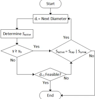
3.4 Diameter Selection Procedure . . . 44
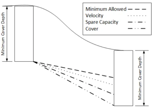
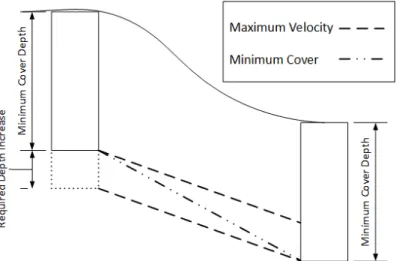
3.5 Cover Slope Exceeds Maximum Velocity Slope . . . 46
3.6 gure . . . 47
3.7 gure . . . 49
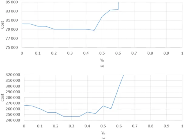
3.8 Sensitivity of γb for (a) Case Study 1 and (b) Case Study 2 . . . 53
4.1 Example network . . . 68
4.2 Example Network Iteration Selections . . . 69
4.3 Node Permutation Restriction Example . . . 75
5.1 Simultaneous Optimization Model . . . 79
5.2 Example Network 1 . . . 82
5.3 Example 1: Fitness progression of the best solution . . . 83
5.4 ACO-TGA Solution of Example 1 . . . 84
5.5 Eect of Fitness Warping . . . 84
5.6 Example Network 2 . . . 84
5.7 Example 2: Fitness progression of the best solution . . . 84
5.8 Direct-Edge Solution of Example 2 . . . 85
5.9 Example Network 3 . . . 86
5.10 Example 3: Fitness progression of the best solution . . . 87
5.11 Perm-Edge Solution of Example 3 . . . 87 ix
6.1 Irregular Manhole Shifting . . . 92
6.2 Example Base Graphs . . . 93
6.3 Shape Functions used for Terrain Generation . . . 93
7.1 Example Network . . . 100
7.2 Elevation Rank . . . 102
7.3 Distance Ranks . . . 103
7.4 Distribution of Slopes . . . 105
7.5 Betweenness Centrality Distribution . . . 106
7.6 Diameter Distribution . . . 107
7.7 Reingold Tilford Tree Layout . . . 109
7.8 Elevation Rank Heuristic Distribution . . . 110
7.9 Progression of Best Solution Cost . . . 112
7.10 Progression of Elevation Rank Prominence . . . 113
7.11 Progression of Elevation Rank Average Dierence . . . 114
7.12 Progression of Elevation Rank Dierence Standard Deviation . . . 115
7.13 Progression of Distance Rank Average . . . 115
7.14 Progression of Distance Rank Standard Deviation . . . 116
7.15 Progression of Maximum Distance Rank . . . 116
7.16 Progression of Average Slope . . . 117
7.17 Progression of Slope Standard Deviation . . . 118
7.18 Progression of Maximum Slope . . . 118
7.19 Progression of Graph Degree Centrality . . . 119
7.20 Progression of Average Betweenness Centrality . . . 119
7.21 Progression of Betweenness Centrality Standard Deviation . . . 120
List of Tables
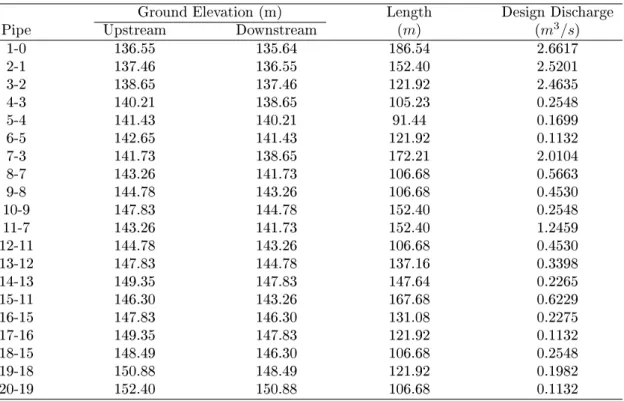
3.1 Data of Case Study 1 . . . 48
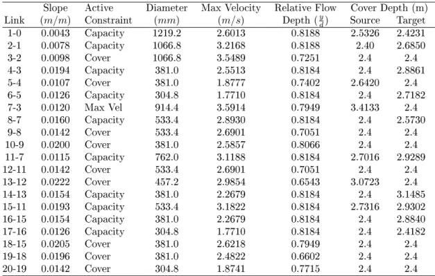
3.2 Results of Case Study 1 . . . 49
3.3 Heuristic Solution of Case Study 1 . . . 50
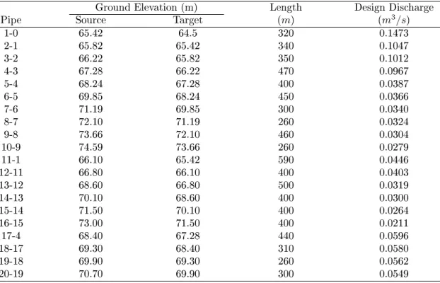
3.4 Data of Case Study 2 . . . 51
3.5 Results of Case Study 2 . . . 52
3.6 Heuristic Solution of Case Study 2 . . . 52
5.1 Example Network 1 Parameters and Results . . . 83
5.2 Example Network 2 Parameters and Results . . . 85
5.3 Example Network 3 Parameters and Results . . . 87
6.1 Base Hydrograph . . . 96
6.2 Flow Rate Scale Factors . . . 97
6.3 Pipe Variations . . . 97
8.1 Results of Bilinear Topography . . . 126
8.2 Results of Hill Topography . . . 128
8.3 Results of Bowl Topography . . . 129
8.4 Results of Concave Topography . . . 130
8.5 Results of Convex Topography . . . 131
8.6 Results of Flat Topography . . . 132
8.7 Results of Simplex Noise Topography . . . 133
8.8 Combined Results of all Topographies . . . 134
8.9 Base Performance by Generation . . . 135
8.10 Best Heuristic Performance by Generation . . . 136
Chapter 1
Introduction
The South African Human Rights Commission, in their report entitled "Water is Life. Sanitation is Dignity: Accountability to people who are Poor" (Ramkissoon, 2014) argues that access to decent sanitation services and infrastructure is a human right. They investigated the nancial and technical requirements of delivering basic sanitation to an estimated 5.2 million people still lacking such services in South Africa alone. It is stated that an estimated R44.75 billion is required to provide basic services, while R31.25 billion is needed to refurbish and upgrade existing infrastructure. In stark contrast to these amounts, the South African budget allocation for sanitation was approximately R3.2 billion nation wide. This state of aairs is not limited to South Africa alone. In an article titled "A Place to Go", National Geographic Magazine (Royte, 2017) reports that an estimated 950 million people currently defecate in the open worldwide.
Towards alleviating this public health hazard, it is clear that money allocated to the provision of sanitation services has to be spent as eectively as possible. This statement is true for all civil engineering endeavours and engineers often pride themselves for being able to rise to this challenge. The collective eorts and experience of past and present engineers have lead to modern design principles and techniques which do, most often, provide very good designs and in some cases even optimal designs. However, some problems in the engineering domain are categorized as NP-Hard (Knuth, 1974; Leeuwen, 1998). NP-Hard problems are decision based and the number of possible solutions grow exponentially relative to the size of the problem. Even the most experienced engineers, relying on a combination of intuition, experience and experimentation, can only consider a trivially small subset of the possible solutions to such problems.
The rapid increase in digital computing power, paired with the development of techniques capable of exploiting that power to address NP-Hard problems, have in the last two decades opened up exciting possibilities in engineering design. It is within this domain that the research described here aims to make a contribution.
1.1 Overall research objective
Many techniques have been developed, both recently and in the past, to optimize the design of sewer networks. Sewer network optimization requires the solution of two problems. The rst is to determine an optimal layout of the network compo-nents, referred to as layout optimization. The second is to determine the optimal hydraulic characteristics of any given layout, referred to as hydraulic optimiza-tion. Most existing optimization algorithms focus exclusively on the hydraulic optimization part, while the layout remains static (Lejano, 2006). Recently, how-ever, promising algorithms have been developed which aim to solve both problems simultaneously, for example Moeini and Afshar (2012).
Given the enormous need for sanitation services, the nancial constraints in-herent to providing it, and inspired by technical advances like Moeini and Afshar (2012), the overall research objective is to develop new techniques to minimise the capital expenditure required for the installation of sewer networks. The aim is not only to improve on existing algorithms. While addressing their shortcomings, new approaches and test cases are developed which enable a thorough investigation into the nature of the optimality of sewer network designs. Changes in network layout parameters during optimization are monitored and their eects on the cost of the solution are determined. This knowledge is then exploited to modify the proposed algorithms in order to further improve their behaviour.
The broad scope of the stated objective is limited and focussed in the overview of the dissertation chapters presented below.
1.2 Document Structure
While it is common for theses and dissertations to present a complete overview of the relevant literature and problem aspects early on, this document does not. The research described here employs a broad set of techniques across many dierent elds of engineering, computer science and mathematics. To present the reader with all the relevant information of each facet, out of context of the ow of the investigation, is deemed detrimental to the readability of the document. The con-clusions reached at each stage of the investigation often to lead to a natural next step in the process, which only becomes obvious at that stage. For example, a discussion of "simplex noise" and its role in the development of a problem library (cf. Chapter 6) does not oer the reader much insight at this stage. Its application only becomes clear once the need to generate specic topographies for sewer net-works has been motivated, which in turn only becomes clear once the results of the simultaneous optimization algorithms (cf. Chapter 5) have been discussed. Con-sequently, comprehensive literature reviews, problem statements and discussions
of relevant techniques are included in each chapter, as described below.
1.2.1 Chapter 2: Sewer Network Design as an
Optimization Problem
The reader is introduced to sewer network design from an optimization perspec-tive. The focus is on presenting a clear understanding of the problem which is to be solved and the key aspects which will be focussed on by proposed solutions. Additionally, the objective function of the optimization is presented. Design con-straints, such as minimum and maximum ow velocities, to which any solution will be subject are presented and their inclusion motivated. Analysis and design equations that incorporate the constraints are presented and their use motivated. Simplifying or limiting assumptions made during the design procedure are intro-duced, discussed and motivated. Signicant shortcomings in existing optimization approaches are highlighted and the methodology to overcome them is described and motivated.
1.2.2 Chapter 3: Hydraulic Optimization
Chapter 3 focusses exclusively on the hydraulic optimization problem, i.e. deter-mining the optimal set of hydraulic parameters for a given layout. A comprehensive overview of existing hydraulic optimization techniques is given and their shortcom-ings are noted and discussed. A new algorithm, which relies on minimum slope information to perform near optimal diameter selections with very little compu-tational eort, is presented. The new algorithm, denoted Heuristic Optimization by Minimum Slopes (HOMS), is applied to two case studies and its results and computational performance are compared to current state of the art solutions.
1.2.3 Chapter 4: Layout Optimization
This chapter focusses exclusively on the layout optimization problem. A com-prehensive review of existing sewer network layout creation strategies and op-timization algorithms is presented. New layout creation strategies, with varied characteristics, are presented and Ant Colony Optimization (ACO) is employed to perform optimization of the layouts they produce. An overview of the basic ACO algorithm is given, and modications made to it are discussed and motivated.
1.2.4 Chapter 5: Sewer Network Optimization
In this chapter the HOMS algorithm of Chapter 3 is combined with the layout optimization algorithms of Chapter 4 to form hybrid algorithms capable of solving
both sub-problems simultaneously. Three example problems are presented. The new algorithms are used to solve each of the example networks and the results are compared to references from literature. Key areas of interest are identied and motivated for further investigation.
1.2.5 Chapter 6: Standard Problem Library
The results of Chapter 5 indicate that a thorough study of algorithm behaviour for problems with specic characteristics will be benecial. This chapter describes the development of software which is capable of generating sewer network instances with controllable characteristics, for example the number of manholes in the net-work, the average length of pipes, etc. Through combinations of network char-acteristics, 153 classes of sewer network problems are dened. The software is then used to generate 20 instances of each class, resulting in a total of 3060 sewer network instances. These instances can be used as a standard library to evaluate the performance of optimization algorithms when exposed to the dierent problem classes.
1.2.6 Chapter 7: Characteristics of Optimal Networks
The question why do particular algorithms perform better for certain problems than others, is investigated. The aim is not simply to determine which algorithm characteristics yielded better solutions, but rather to determine what characteris-tics were displayed by the best solutions.
Based on this, network parameters are proposed which oer insight into the characteristics of a specic layout. The algorithms developed in Chapter 5 are then used to solve each of the 3060 problems generated in Chapter 6 multiple times. During execution of the optimization algorithms the proposed network parameter values are captured at regular intervals. The associated characteristics are compared to the cost of the network at the respective intervals and used to establish correlations between network characteristics and cost.
Using the established correlations, heuristic inuence factors are proposed which guide the ACO algorithms towards decisions which more strongly favour or avoid desired or undesired characteristics respectively. The eect of each heuristic inuence on the network characteristics are carefully monitored to ensure they operate as far as possible on the desired characteristic alone. Due to the interde-pendent nature of sewer network characteristics some side eects are unavoidable.
1.2.7 Chapter 8: Augmenting Sewer Network Optimality
to the algorithms of Chapter 5. The modied algorithms are used to solve each of problems from the standard problem library again. The results are presented compared to the unaltered state of the algorithm. Furthermore, the best perform-ing heuristic inuence factor or combination of factors at varyperform-ing stages of the algorithm's execution are also presented.
1.2.8 Chapter 9: Conclusions and Recommendations
Chapter 9 summarises the important results and conclusions of each chapter. A critical evaluation of contribution of each chapter is included. Recommendations and guidelines for further research are discussed.
Chapter 2
Sewer Network Design as an
Optimization Problem
In this chapter an overview of gravity sewer network design relevant to the op-timization problem is presented. In this investigation the sewer networks under considerations are limited to only gravity sewer networks with no special struc-tures, such as rising mains or pump stations, present and no divergent structures. These restrictions are motivated where relevant to the sewer network design aspect currently under discussion. The mathematical modelling of the two sub-problems of sewer networks as used in this investigation are introduced. The cost function used to determine a unit capital cost associated with a complete design throughout this investigation is introduced.
The design of sewer networks consists of two parts: rstly a suitable layout, taking into account existing or planned infrastructure, such as roads or buildings, has to be determined. Secondly the hydraulic design has to be performed to deter-mine cumulative ow rates, pipe diameters, cover depths and ow velocities. The hydraulic analysis model used to calculate cumulative ow rates is introduced and its use motivated. The reader is introduced to the Fitness Warping phenomenon present in some simultaneous sewer network optimization algorithms.
2.1 Calculating Network Cost
The design is to be optimized, in this investigation, in terms of capital-investment cost. The necessary steps to calculate an accurate estimated construction cost for a complete sewer network is a strenuous and complex task. To calculate an accurate estimate in real currency of the capital-investment cost of a network re-quires an abundance of information, such as cost of excavation rates which take soil conditions into consideration, the cost of network elements such as pipes or
manholes, labour expenses, etc. The list is truly enormous. An accurate estima-tion of capital expenditure is the concern of the contractor once a detailed design has been completed. Furthermore, the cost-rates used for the dierent aspects of construction are often well guarded due to the competitive nature of the tendering process in construction. Consequently, automating an accurate real-currency cost estimation of a complete sewer network is beyond the scope of this investigation.
Instead, functions have been formulated in the literature which allow a unit cost value to be calculated. These functions approximate the expected real-currency cost, based on the most capital intensive variables i.e. soil excavation and pipe diameters. It is important to note that for the purpose of optimization accurate costs are not required. Rather, the calculated costs for a multitude of network de-signs should be correct relative to one another. That is to say, if the real-currency estimated cost of Network A is higher than that of Network B, then the approx-imate unit cost function should deliver the same result if not necessarily by the same ratio. If a cost function has this property it allows an optimization algorithm to select the correct network as the least or less expensive option correctly and consistently. The formulation and testing of such a cost-function is beyond the scope of this investigation. A Cost function, which uses interchangeable unit val-ues, is taken from the literature (Moeini and Afshar, 2012) which allow accurate relative comparison between examples for the purpose of optimization.
2.1.1 Capital-Investment Cost Function
The function used to calculate the capital-investment is as used by Moeini and Afshar (2012): C = N X i=0 LiKi(di, Eiave) + M X j=0 Kj(hj) (2.1) Where:
C = Cost Function of Sewer Network
Li = The length of pipe i, i∈ {1, ... , N}
Ki = Unit cost function of pipe i, dened in terms of its diameter (di) and average cover depth (Eiave)
Kj = Unit cost function of manhole j, dened in terms of its height (hj)
N = The number of pipes in the network
Figure 2.1: Denition of Depth Variables
Figure 2.1 shows the denition of depth variables used in the cost function, as well as throughout the entirety of this investigation.
This function is dependent on unit cost functions which may be modied for a specic problem to more accurately represent the expected cost for the network.
2.1.2 Unit Cost Functions
In this investigation the majority of problems under consideration are theoretical. Consequently, the unit cost functions do not require adjusting based on the prob-lem. The only constraint is that the same unit cost functions be used for networks which require their costs to be compared, assuming the unit cost function produce accurate relative costs. Similarly to the cost function, the derivation of the unit cost functions is beyond the scope of this investigation. Two unit cost functions are used in this investigation. The rst is used for all problems excluding a single benchmark problem where dierent unit cost functions have to be used to allow direct comparison of results from previous investigations. Both sets of unit cost functions are introduced here.
The rst set of unit cost functions are as used by Afshar et al. (2011), as shown below.
Kj = 41.46hj (2.3) Where:
di = The diameter of pipe i [m]
Ei = The average cover depth of pipe i [m]
hj = The height of manholej [m]
These are exponential unit cost functions dependent on the diameter of a pipe, its excavation depth and the excavation depth of a manhole. Intuitively, the expo-nential growth in cost of a pipe as its diameter and excavation depth increases is sensible. Furthermore, the unit cost a pipe has a term which depends on both pa-rameters simultaneously which takes into account the increased excavation width for a larger diameter. The unit cost function for a manhole is a linear function de-pendent only on the excavation depth. These unit cost functions are used through-out the investigation, excluding one benchmark problem in Chapter 3 where it is stated again.
The second set of unit costs functions are proposed by Meredith (1972), as shown below. Ki = 10.98d+ 0.8E−5.98 if d ≤3f tand E≤10f t 5.94d+ 1.166E+ 0.504Ed−9.64 if d≤3f t and E>10f t 30.0d+ 4.9E−105.9 if d>3f t (2.4) Kj = 250 +h2m (2.5) Where:
d =The diameter of pipei [f t]
E =The average cover depth of pipei [f t]
hm =The height of manholem [f t]
The unit costs proposed by Meredith (1972) are calculated using imperial unit val-ues. The unit cost of a pipe presented by Meredith (1972) takes into account the variation in expected cost as excavation depths and diameter increases occur and dene a step-wise bi-linear function rather than an exponential function. Further, the unit cost of a manhole increases exponentially rather than linearly. These unit costs are only used during the evaluation of the proposed hydraulic optimization procedure of Chapter 3 to allow direct comparison of results.
2.1.3 Formulating the Objective Function
All optimization algorithms require an objective function by which to evaluate the tness of a solution. In this investigation, as stated previously, the objective is to minimize capital-investment cost. Consequently, the objective function is:
M inimize C = N X i=0 LiKi(di, Eiave) + M X j=0 Kj(hj)
where all variables are as dened for Equation 2.1. This objective function is subject to a multitude of constraints discussed later in this chapter, which may be violated by a given solution. It is common practice in the use of optimization algorithms to use a penalized version of the objective function to account for the violation of constraints:
M inimize P = C + αX
i
gi (2.6)
Where:
P =The Penalized Objective Function
C =Cost of the Sewer Network, Equation 2.1
gi =Violation value of constraint i, 0 if unviolated
α =A suciently large constant so ensure feasible
solutions have a better tness than infeasible
solutions, i.e. solutions that violate one or more constraints
It is important not to discard infeasible solutions from a meta-heuristic algorithm as, especially early on, the algorithm may struggle to nd the feasible region of the search space and will be required to learn from infeasible regions. Furthermore, an infeasible solution may be right on the edge of the feasible search space which is adjacent to the optimal valley or peak of the search space. If this solution is discarded the algorithm cannot learn from this solution, despite how close to the optimal solution it is. The penalized objective function allow infeasible solutions to contribute to the progression of the meta-heuristic algorithm while ensuring it will never be considered a better solution than a feasible solution ifαis suciently
large. Note the contribution of the second term of Equation 2.6 is0if no constraint
is violated. Equation 2.6 is used throughout this investigation as the objective function.
2.2 Layout Design
Layout design of sewer networks is again a two part problem. The rst is to determine the spatial location of manholes and pipes. The second is to determine the direction of ow of each pipe. Only once both parts of the problem have been solved is a full network layout found.
2.2.1 Spatial Design of the Network
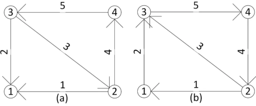
Referring to Figure 2.2. The nodes, representing manholes labelled 1, 2, 3 and 4 respectively, are connected by edges, representing pipes labelled 1, 2, 3, 4 and 5 respectively.
Figure 2.2: Layout Design Example
In this example the spatial position of the manholes and pipes have already been determined, i.e. the rst part of the design is complete. However, it may have been equally feasible to place the manholes at dierent locations and to connect them dierently, for example by placing pipe 3 between manholes 1 and 4 rather than 2 and 3. This part of the design, deciding on the spatial location of manholes and how to connect them with pipes, is most often governed by existing or planned infrastructure, such as roads or buildings, and topographical considerations, such as hills or steep inclines. In this investigation it is assumed that the positioning of manholes and pipes is completed prior to the optimization process aimed at minimizing the installed cost of the sewer network. The positioning of manholes and pipes is referred to as the base layout, or base graph, of the layout. All pipes and manholes included in the base graph must be present in the nal solution. The base layout is modelled mathematically as an undirected graph where the vertices
represent manholes and the edges pipes: Gbase = (V, E)
Where:
Gbase = The base graph
V = The vertex set, whose elements are the vertices of Gbase which represent manholes of the sewer network
E = The edge set, whose elements are the edges of Gbase
which represent pipes of the sewer network. As the graph, Gbase, is undirected the individual edges are undoredered pairs (u , v) where
u and v are vertices in V
2.2.2 Directional Design of the Network
The second part of the layout design is to determine the direction of ow for each pipe. This part of the layout design is deceptively complex and the number of possible permutations grows exponentially as the number of vertices and edges present in the base graph increases. This part of the layout design is the concern of the optimization procedures which are discussed in detail in Chapter 4; A brief overview of the required decisions to complete the directional design is given here. Figure 2.3 shows two directional graphs, directions are indicated by arrows. Figure
Figure 2.3: Directional Layout Design Examples
2.3 shows two feasible nal layouts, of a possible 52 = 25, of the base layout
shown in Figure 2.2. The choice of ow directions can heavily inuence the nal capital investment cost of the completed sewer network, especially when adverse
topographical conditions are present. If, for example, manhole 2 has a much lower elevation than manhole 3 then using sound engineering intuition we can readily observe that the design of Figure 2.3 (a) requires less excavation than that of Figure 2.3 (b). This reduction in required excavation can be expected to lead to a reduction in capital expenditure. However, the problem becomes increasingly dicult as the size of the base graph increases, since the change in ow direction of a single pipe may have signicant eects on the cumulative downstream ow rates within pipes and therefore their required diameters and slopes.
Notice that in both designs of Figure 2.3 cycles are present in the nal layout designs. For Figure Figure 2.3 (a) the cycle 2-4-3 exists and for Figure 2.3 (b) the cycle 2-3-4 exists. As stated before, in this investigation only gravity sewer networks are considered with no special structures present.
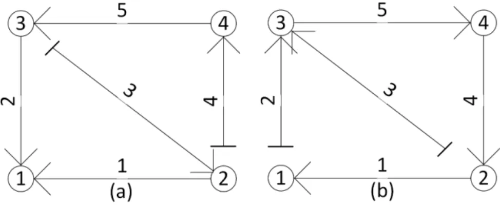
Figure 2.4: Directional Layout Design Examples With No Cycles
Moeini and Afshar (2012) propose disconnecting pipes from their upstream manholes and creating what they term adjacency nodes, which are created arti-cially for purpose of the optimization at the same location as the existing upstream manhole. The practical implication of this is that the pipe has no upstream inow from the manhole, and cycles are removed from the network. Referring to Figure 2.4, the networks shown are similar to those in Figure 2.3. In this case, however, the pipes have been disconnected from their upstream manholes and adjacency nodes created, indicated by perpendicular lines on the upstream end of the pipe.
2.2.3 Layout Constraints on the Optimization Problem
As stated previously the layout optimization procedures in this investigation are only concerned with the directional design of the network, the spatial design is
completed a-priori. It is also assumed that all elements present in the base layout have to be included in the nal layout design, with no cycles present. Cycles are avoided through the use of adjacency nodes. How the adjacency nodes are selected is the concern of the layout construction algorithm and described in Chapter 4 of this document. When constructing a network layout the single out-degree con-straint is introduced. The single out-degree concon-straint limits the network such that all manholes may only have a single outlet pipe. This simultaneously avoids cycles and diversion structures within the network. The resulting layout produces a simple branched gravity sewer network with no special structures. Addition-ally, pumping stations are excluded from all networks. These constraints on the layout drastically simplies the hydraulic analysis of the network. This reduction in hydraulic analysis complexity allows greater focus on the layout design prob-lem, which is a key concern of this investigation. Furthermore the restriction on diversion structures and pumping stations is not considered to be severe. It is pos-tulated that these structures decompose a network into a number of sub-networks, each of which can be designed using the techniques developed here.
2.2.3.1 Branched Network Layout
Only gravity sewer networks are considered and no divergence structures are al-lowed in the network. This implies that all manholes may only have a single outgoing pipe.
To ensure that any proposed layout adheres to these simplications, only branched network layouts are selected from the power set of the base layout, which contains all possible looped and branched layouts. Mathematically the restrictions for a branched layout in a network withM manholes are (Moeini and Afshar, 2012):
Xjl+Xlj = 1 ∀j, l ∈ {1, ..., M} M X l=0 Xjl = 1 ∀j ∈ {1, ..., M} (2.7) Where: Xjl = (
1 if an edge with ow from j tol exists
0 otherwise
j: M X l=0 XljQlji − M X l=0 XjlQjli = 0 ∀j ∈ {1, ..., M} ∧ j 6= s (2.8) Where:
Qlji =ow rate in pipe i between nodes l and j
with either node as source or target
s =the outlet node
All networks are dened with a single outlet in this investigation. The conti-nuity equation is not enforced at the outlet since only the inow is modelled for the outlet node. Note that this restriction does not aect the generality of the proposed layout creation algorithms as the same method may be applied for mul-tiple outlets simultaneously. The exclusion of pumping stations is not modelled mathematically as this constraint is simply enforced by exclusion.
2.3 Hydraulic Design
The hydraulic design of a sewer network can only be completed once a complete spatial and directional layout design has been obtained. Furthermore, the suit-ability of any set of hydraulic parameters for a design is dependent on the layout as the layout inuences the cumulative downstream ow rates which in turn af-fect other design variables such as pipe diameter and slope. The hydraulic design requires many variables to be solved simultaneously, such as cumulative down-stream ow rates, diameters, slopes, excavation depths, manhole depths, and ow velocities. All of these variables are subject to design constraints, such as maxi-mum ow velocities or minimaxi-mum cover depths, which ensure the completed design adheres to sound engineering guidelines and regulation codes. Further, there are hydraulic design variables which have to be determined a-priori. This section is not intended to give a comprehensive overview of sewer network design, rather the relevant constraints to the optimization problem are presented.
2.3.1 A-Priori Design Parameters
There are two variables relevant to the hydraulic design which have to be deter-mined a-priori to the design phase. The variables and some practical considerations are discussed here.
2.3.1.1 Ground Elevations
The ground elevation at manholes has to be determined a-priori by land surveyors or GIS systems. There is no alternative way to calculate elevations if an accurate representation is to be obtained. It is assumed that the slope of ground elevations between manholes is linear. While this is perhaps not strictly correct, it is reason-able to assume that the spatial design would not include a pipe which runs through a hill or other adverse topographic occurrence which would require a signicant increase in excavation from the linear assumption.
2.3.1.2 Inow Rates
The expected inow rates into the sewer network due to service connections or ow contributions from an existing network have to be determined a-priori. Inow rates are assumed to enter a pipe at its upstream manhole, consequently the inow hydrographs are assigned at manholes. The expected inow rate due to service or other connections is specied as 24-hour hydrographs.
2.3.2 Hydraulic Constraints on the Optimization Problem
Sewer network design is subject to a multitude of hydraulic constraints of varying complexity. These constraints ensure the completed design can meet the required design ow rates, protect the network from failure and address some obvious health and safety concerns associated with raw sewage contaminating the soil. The design constraints are motivated and formulated mathematically below as part of the optimization problem.
2.3.2.1 Cover Depth
Both minimum and maximum cover depth constraints are enforced. Minimum cover depths protect pipes from imposed loads, such as vehicle loads where sewer pipes pass under roads. The minimum cover depth also prevents cross contam-ination between water distribution networks by ensuring sewer pipes are placed below water mains. Furthermore the minimum cover depth ensures an adequate drop for house connections.
Similarly, the maximum cover depth prevents pipe failure under excessive soil and imposed loads. Maximum cover depth may also be enforced to avoid excessive excavation, specically where soil conditions are adverse.
Where:
Ei = The cover depth of any pipe i at its source or target node
Emin = The minimum allowable cover depth
Emax = The maximum allowable cover depth 2.3.2.2 Velocity
Both minimum and maximum velocity constraints are enforced at the peak design ow rate. The minimum velocity prevents the deposition of solid particles within pipes and manholes. The maximum ow velocity is enforced to prevent erosion of the pipe material.
vmin ≤vi ≤vmax ∀i∈ {1, ..., N} (2.9) Where:
vi = The velocity in pipe iat the peak design ow rate
vmin = The minimum allowable velocity
vmax = The maximum allowable velocity 2.3.2.3 Slope
A minimum slope is enforced on all pipes. This is to prevent inaccurate placement during construction or adverse slopes resulting from pipe settlement. The mini-mum slope requirement also ensures that during full ow conditions the minimini-mum ow velocity is achieved.
Smin ≤Si ∀i∈ {1, ..., N} Where:
Si = The slope of pipe i
Smin = The minimum allowable slope 2.3.2.4 Required Spare Capacity
A percentage spare capacity is enforced at peak ow conditions to ensure that pressurised ow does not occur. The constraint has the additional benet of pro-viding a margin of safety if storm water ingress is experienced during peak ow
times.
Some investigators (Moeini and Afshar, 2012; Haghighi and Bakhshipour, 2015), use a maximum relative ow depth constraint rather than percentage spare ca-pacity. This is merely a dierent formulation of the same constraint. Moeini and Afshar (2012) enforce a minimum relative ow depth. In this implementation no such constraint, or an equivalent, is enforced. This constraint is not common en-gineering practice, furthermore near the sources of the network it becomes almost impossible to enforce this constraint due to unavoidable low ow rates.
SC = Qf ull−Qpeak
Qf ull Where:
SC = Spare Capacity ratio
Qf ull = The full ow rate [m3/s]
Qpeak = The partially full ow rate at peak conditions [m3/s]
This constraint results in partially full ow conditions in all pipes. To solve for the hydraulic parameters Manning's equation is used to estimate velocities throughout this investigation. Qi = 1 ni A 5 3 i P 2 3 i p Si ∀i∈ {1, ..., N} (2.10) Where:
Qi = The ow rate of pipe i
Ai = The area of ow in pipe i
Pi = The wetted perimeter of pipe i
N = The number of pipes in the network
ni = Manning's roughness coecient 2.3.2.5 Commercially Available Diameters
Diameters may only be selected from a discrete set of commercially manufactured diameters.
di ∈ {D} ∀i∈ {1, ..., N} (2.11) Where:
di = The diameter of pipei
{D} = The set of commercially available
2.3.2.6 Progressive Pipe Diameters
The diameter of a pipe may only be equal to or larger than any of the pipes directly preceding itself. This is to prevent possible blockage, damming of waste water and sudden increase in ow velocities in the network.
di ≥ {D}i ∀i∈ {1, ..., N} (2.12) Where:
{D}i = The set of directly preceding diameters of pipe i
2.3.2.7 Progressive Pipe Depths
The outow pipe of any manhole may not be placed above the deepest inow pipe. This prevents permanent damming of waste water and solid deposition in the manhole.
ECi ≥ {EC}i ∀i∈ {1, ..., N} (2.13) Where:
ECi = The excavation depth of the outgoing pipe
i at the node
{EC}i = The excavation depths of all incoming pipes at the source node of pipe i
If all of the above constraints are met a completed design is considered feasible.
2.3.3 Calculating Cumulative Downstream Flow Rates
Inow rates due to service and other connections are assigned at the upstream manhole of a pipe as a 24 hour hydrograph as stated in Section 2.3.1.2. The ow rates need to be routed downstream to the outlet manhole. There are many tech-niques to calculate the downstream cumulative ow rates. Depending on what is required, dierent techniques of varying complexity can be used to obtained the required level of accuracy. van Heerden (2014) compares three alternative hydraulic analysis models for sanitary sewer systems, namely the (i) contributor hydrograph, (ii) kinematic wave and (iii) fully dynamic wave models. In his inves-tigation van Heerden (2014) found that the suitability of a model is dependent on the phase of the engineering process it is applied to. He refers to three phases of the engineering process: planning, design and evaluation. In this investigation the solutions fall within the planning phase. van Heerden (2014) found that during
the planning phase the level of accuracy required is not such that the shortcom-ings of the contributor hydrograph model severely impact on the relevant design variables obtained, most notably for this investigation the peak cumulative down-stream ow rates. Consequently the contributor hydrograph model is used here as it is the least complex of the three models and has the lowest computational complexity, making it ideal for combination with optimization algorithms where computation time can be a limiting factor. A brief overview of the contributor hydrograph model is presented.
2.3.3.1 Contributor Hydrograph Model
The contributor hydrograph model was rst introduced by Shaw (1963). Later, Stephenson and Hine (1982) found that ordinary time-lag routing, used in contrib-utor hydrographs, is of sucient accuracy for sewer network design purposes. van Heerden (2014) found that it was indeed sucient if the design is in the planning phase, as is the case in this investigation. In the contributor hydrograph model inow rates are dened as 24 hour hydrographs. The inow hydrographs are de-ned by parameters associated with the land use of the service connections and the number of units serviced. In this implementation the local inows are calculated from South African standard unit hydrographs associated with a specic landuse. The unit hydrographs are included in Appendix A. The local inows for each of the landuses is summed to give the total local inow to the pipe, which is assigned at the upstream manhole.
Qt= n X i=0 EELU i×(U HLU it ×PLU i+LLU i) (2.14) Where:
Qt = Local inow at time t
n = Number of considered land uses
EELU i = Number of land parcels with land use i
LLU i = Leakage for land use i
PLU i = Peak for land use i
U HLU i = Unit Hydrograph for land use i
Peaks of hydrographs are shifted and the accumulated ow attenuates as the ow is routed downstream. This is due to the considered time delay of ow to reach downstream manholes. Time delay is calculated using Manning's equation at full ow conditions. Calculating time delay at full ow conditions produces a
conservative estimate of time delays while greatly reducing computational eort as determining the depth of ow in the pipe is not required.
Time Delay = t = L
v
Velocity = v = Qf
Af
Full Flow Rate = Qf =
1 n A5f/3 Pf2/3 √ S (2.15)
Because of time delay eects the accumulated ow rates cannot be directly summed. Once a hydrograph has been shifted due to time delay the ow values are no longer known at the downstream time steps of the hydrograph where ow rates are known. If, for example, after shifting a hydrograph's peak is at hour 4.5, and the inow is required at hours 4 and 5 then the peak will be lost at the downstream summation. A conservative linear interpolation method is used for peak shifting to ensure maximum ows are always simulated. Figure 2.5 shows the hydrograph coordinates during interpolation.
Figure 2.5: Hydrograph Interpolation Points
The procedure to calculate the shifted ow rate at time T is as follows: 1. The rst point (T1, Q1), before time T is found
2. The second point (T2,Q2), following time T is found 3. The third point (T3, Q3), following timeT2 is found
4. if Q2 > Q1 and Q2 > Q3, the peak ow rate, Q2, is shifted to time T. 5. else, the resultant ow at time T is equal toQ1 + t(Q2 − Q1).
Figure 2.6 shows the 24 hour composite hydrograph of a single very high income residential unit, as well as a shifted hydrograph. To calculate the time delay a diameter of 0.16m, slope of 0.013m/m, Manning roughness coecient of 0.012
and a pipe length of 200m was used.
Figure 2.6: Time Shifted Hydrograph
To calculate the time delay the full ow rate is required. Using equations 2.15 the full ow rate may be calculated as Q = 0.0223m3/s, the ow velocity, v, is then 1.1113m/s resulting in a time delay, t, of 180s. Referring to Figure 2.6, the
peak before shifting is at hour 8. Once the time delay of180s is included the peak
falls at hour 8.05, similarly all other known values are moved 0.05forward. If this
hydrograph is to be added to a downstream manhole the values at the original time intervals have to be calculated. The calculation of the shifted ow rate value at hour 7, the time T, is shown below following the method above:
1. Find the rst point (T1, Q1), before time T. Select T1 as hour 6.05 of the attenuated hydrograph, whereQ1 = 1.39l/s.
2. Find the second point (T2, Q2), after time T. Select T2 as hour 7.05 of the attenuated hydrograph, whereQ2 = 1.95l/s.
3. Find the third point (T3, Q3), after time T2. Select T3 as hour 8.05 of the attenuated hydrograph, whereQ3 = 1.73l/s.
4. Q2 = 1.95l/s > Q1 = 1.39l/s and Q2 = 1.95l/s > Q3 = 1.73l/s. The ow rate at time T = Q2 = 1.95l/s.
This procedure is repeated for each time step of the hydrograph and the complete shifted hydrograph obtained which may be summed with the downstream ow rate to determine the cumulative ow rate. Note that the peak is shifted to an earlier rather than later time despite being delayed. van Heerden (2014) noted that the contributor hydrograph model does not accurately determine the expected time of a peak ow rates, though the value of the peak ow rate is determined accurately. For this investigation, the time of the peak ow rate is not relevant, the important factor is that the peak value is correct to allow accurate calculation of the other hydraulic design variables. If, once the algorithms described in this section has completed a preliminary design, more accurate hydraulic calculations are required the proposed design can be transferred to a hydraulic analysis package more suited to the requirements of the design.
2.4 Fitness Warping
As mentioned before sewer network optimization consists of two sub-problems which must be solved simultaneously. To this eect many algorithms have been developed, as will be discussed later in Chapters 3 and 4. Many of the algorithms approach this problem by determining both the layout and element size character-istics simultaneously, i.e. element sizes are selected before a complete layout has been found and hydraulic analysis is possible. While at rst this approach appears to be sound there is a critical phenomenon present that warrants caution: Fitness Warping.
Fitness warping, dened here for the rst time to the best of the author's knowledge, refers to the skewed tness value associated with a good layout when accompanied by poor element sizes. Because the element sizes are far from opti-mal for the layout, the entire tness of the solution will be deemed poor and the algorithm unable to recognize that a good layout has been found. This eect is most severe in the early stages of the optimization where layouts and element sizes are still selected at random as the driving mechanism of the algorithm has not had sucient time to learn from previous solutions.
This phenomenon is not unique to sewer networks, but may be present in any optimization problem where two or more sub-problems are solved simultaneously. Researchers have applied optimization techniques and successfully avoided tness warping to a variety of problems. Giustolisi and Savic (2006) developed a hybrid regression method that combines genetic algorithms with conventional numerical regression techniques. Haghighi and Bakhshipour (2015) use a complex Tabu-Search model combined with a loop-by-loop cutting algorithm (Haghighi, 2013) to
determine sewer network layouts and an adaptive genetic algorithm (Haghighi and Bakhshipour, 2012) to determine element sizes for each layout. However, none of the researchers draw specic attention to the phenomenon or attempt to dene and characterise its eects. Here, the phenomenon is actively avoided and the eects demonstrated in Chapter 5 by means of comparison to an algorithm where the phenomenon is present.
To avoid tness warping the optimal set of element sizes has to be determined for each layout. However, determining element sizes is an optimization problem in its own right. Consequently, this approach can become extremely computa-tionally expensive if, for example, metaheuristic algorithms are employed for both sub-problems. For this reason a computationally ecient hydraulic optimization model is developed (cf. Chapter 3). It is combined with a metaheuristic layout optimization algorithm (cf. Chapter 4), so that each individual layout produced by the metaheuristic can be hydraulically optimized and the entire algorithm com-pleted in reasonable time.
2.5 Summary and Conclusions
In this chapter the aspects of sewer network design relevant to the optimization problem were introduced. It was stated that in this investigation the network is to be optimized in terms of capital investment cost. The function used to calculate the investment cost as well as the unit cost functions associated with it were introduced. The use of a penalty function to avoid infeasible solutions was motivated.
The two parts of the layout design problem, spatial and directional layout design, were introduced. Spatial design of the layout is to be completed a-prior to the optimization procedures which are concerned with the directional design of the network. The concept of a base layout, which includes all required manholes and pipes of the nal solution, was described. The design constraints relevant to the layout creation algorithms, namely that no cycles may be present in the nal layout, was reviewed. The adjacency node implementation used by Moeini and Afshar (2012) to avoid cycles in the layout was described.
Constrains on the hydraulic design parameters relevant to the optimization was reviewed and their inclusion motivated. It was stated that the suitability of a given set of hydraulic parameters for a design is dependent on the network layout. The a-priori design variables, namely ground elevations at manholes and inow rates due to service connections, were introduced and the required data format described. The calculation of the downstream cumulative ow rates using the contributor hydrograph model was determined to be suciently accurate for use in the design techniques described here. The method used to attenuate ow rates
with time delay and a conservative linear interpolation procedure to determine intermediate ow values of the hydrographs was introduced.
The tness warping phenomenon of algorithms which select both layout and hydraulic parameters simultaneously was introduced. To avoid this phenomenon, a computationally ecient hydraulic optimization model (cf. Chapter 3) which can be used to optimize the hydraulic parameters of each layout produced by a metaheuristic layout optimization algorithm (cf. Chapter 4) is proposed by this investigation, thus avoiding tness warping.
This chapter did not go into any detail on how the optimization algorithms incorporate the design constraints or how the layout creation algorithms use the concept of adjacency nodes. Rather, the focus was on formulating the problem of sewer network design as an optimization problem.
The process by which an optimized design can be obtained comprises layout optimization and hydraulic optimization for each candidate layout. In chapter 3 the hydraulic optimization procedure is described, followed by the layout optimiza-tion procedure in chapter 4. It should be noted that the hydraulic optimizaoptimiza-tion procedure is useful for any given layout, i.e. it can be used even if no attempt is made to optimize the network layout.
Chapter 3
Hydraulic Optimization
Hydraulic optimization is the component of the sewer network optimization prob-lem in which eprob-lement sizes, installation depths and slopes are determined for a given layout. Due to the highly constrained nature of hydraulic optimization and complexity of simultaneous solution algorithms this part has seen considerably more work than the layout optimization problem (Lejano, 2006). In this chap-ter an overview of the hydraulic optimization problem is presented. The state of the art solutions to the problem are reviewed and their shortcomings, relevant to this investigation, identied. A computationally ecient heuristic optimization algorithm which relies on required slope information to systematically solve for all hydraulic parameters, is developed and applied to two case studies from the literature. It is shown to obtain near optimal solutions while requiring very little computation time.
3.1 Problem Statement
The hydraulic optimization problem can be seen as an element size selection, or pipe diameter selection, problem. While other approaches may be viable, this is certainly the best option as diameters can only be selected from a discrete set of commercially available diameters. The hydraulic optimization problem is catego-rized as a mixed integer linear programming optimization problem.
Referring to Equation 2.10, Manning's equation for open channel ow, it is clear that ow rate, Q, pipe slope, S and diameter, d are dependent variables.
The ow area,A, and wetted perimeter,P, are dependent on the diameter as well
as the ow depth, y, within a pipe. Full ow conditions are often assumed when
performing hydraulic calculations for sewer networks as this greatly simplies the required calculations. All three variables, namely the ow rate, slope and diameter,
have to be determined, either by some mechanism of the optimization algorithm, or by calculation. Most commonly diameters are selected by a mechanism of the optimization algorithm from the discrete set of available diameters. Cumulative ow rates for pipes are often predened in optimization benchmarking problems, so no hydraulic analysis to determine ow rates is required. This only leaves the slope to be determined. As Manning's equation requires the ow area and wetted perimeter the slope can, at this stage, still not be calculated as the ow depth needs to be determined. However, as stated it is common practice to assume full ow conditions and calculate ow area and wetted perimeter based on this as-sumption. This allows calculation of the required slope at full ow conditions. If the assumption of full ow conditions is not made the ow depth within a pipe has to be determined. Calculating the ow depth requires a highly implicit equation in terms of the ow depth to be solved using some form of numerical analysis.
The problem is further complicated if ow rates are not predened and need to be obtained using hydraulic analysis. In this case values for the slopes are often estimated and adjusted if need be after hydraulic analysis. However, it is possible in the case of a branched network layout to perform the hydraulic analysis without the need to estimate slopes as at the upper ends of the network the inow into a pipe is known at the start of the analysis. The hydraulic analysis procedure can thus start at the upper pipes in the network and proceed downstream.
If the hydraulic optimization procedure is to be successful it must overcome all of these challenges simultaneously, with or without assumptions. In this inves-tigation as few as possible assumptions are made during the analysis procedure. Existing hydraulic models are modied or new procedures developed to allow all variables to be calculated accurately from engineering theory and principles rather than to rely on estimations.
3.2 State of the Art
This section describes the most representative hydraulic optimization procedures in the literature and identies shortcomings, within the context of this investiga-tion, of these procedures. A motivation for the development of an algorithm which overcomes the limiting shortfalls of the existing state of the art optimization pro-cedures is presented.
Many optimization techniques have been applied to the hydraulic optimization problem of sewer networks. In the past, dynamic programming methods or even manually manipulable spreadsheets have been developed which were able to nd
very good solutions to problems subject to very strict conditions or limiting as-sumptions. These algorithms will be referred to as the classic algorithms. It should be noted that the review of the classic algorithms is relevant to this study as a similar approach is followed in this investigation albeit signicantly more modern in its implementation. In more recent times, with the emergence and meteoric rise in popularity of metaheuristic algorithms, the hydraulic optimization problem has seen a resurgence in the literature as researchers develop metaheuristic algorithms to solve the problem.
3.2.1 Classic Algorithms
The classic optimization algorithms more often than not relied upon dynamic pro-gramming (DP) or some variation thereof. Dynamic propro-gramming optimizes each individual sub-problem of a larger problem and assumes that these local optima will result in a good, if not globally optimal, solution for the large scale problem. Furthermore, if sub-problems are prone to repetition within a problem the result of a previous solution is stored and called upon at a later time. In the case of sewer networks a typical sub-problem is to select the optimal diameter for an in-dividual pipe, without taking into account the eect this diameter has on up-or downstream pipes. In sewer networks it is very unlikely that the conditions are replicated exactly for two or more pipes, so storing previous solutions may not oer as much value as for other problems.
Mays and Wenzel (1976) applied Discrete Dierential Dynamic Programming (DDDP) to the design of gravity sewer networks with the assumption that the direction of ow is xed, no cycles exist within the network and it operates solely under the eects of gravity. This is similar to the assumptions made in this inves-tigation, and in fact the majority of investigations which came thereafter. DDDP is an iterative procedure which limits the search space to a discrete set. This has some signicant drawbacks. Reducing the search space to discrete partitions re-duces the likelihood of nding the global optimum, furthermore the discrete set for each variable has to be determined manually, thereby reducing its practicality. The algorithms developed by Mays and Wenzel (1976) divides the network into so-called stages using predened isonodal lines between manholes. These isonodal lines are imaginary lines dened by the user which indicates stages. Each stage is solved individually using a recursive equation to determine the optimal drop in crown elevation of a pipe across the stage. At each stage a cost is determined which is analogous to the cost of installing each pipe and constructing the upstream manholes of the respective pipes for each previously completed stage as well as the current stage. This procedure is repeated until the nal result is obtained. The main drawback of the DDDP method is the required user input in dening the
stages and isonodal lines, as well as limitations on the search space, which makes the likelihood that the global or even a good local optimum has been found very slim.
Robinson and Labadie (1981) used a generalized DP package, referred to as CSUDP, to develop an optimization algorithm. Their algorithm allowed a com-bined maximum of 50 manholes and pipes, severely restricting its practical use for modern day applications. Furthermore, their application limited manholes to a maximum of three incoming pipes and one outgoing pipe. Their algorithm divided the network into stages according to pipes. If, for example, two pipes enters a manhole there are two stages associated with the manhole. The state variables of their algorithm is the pipe crown elevation while the decision variable is the pipe diameter. Their algorithm starts at the upstream end of the network and systematically determines the least cost connection at each stage of the problem to eventually nd the best solution.
Miles and Heany (1988) developed a stormwater drainage design method using a spreadsheet package, requiring manual input and manipulation from the user, which may be applied to static layouts. The shortcomings of this method are ob-vious. While their spreadsheet based algorithm did produce very good results the manual manipulation requirement makes its use extremely impractical if the aim, as is the case with this investigation, is to combine the algorithm with a layout optimization procedure.
Some classic hydraulic optimization algorithms have been developed and suc-cessfully combined with layout optimization algorithms. Walters (1985) used a DP algorithm for simultaneous layout and size optimization. The hydraulic optimiza-tion part of the DP algorithm (Walters, 1985) uses a discrete set of pipe sot levels from which to select the up and downstream levels of pipes. Once the sot levels are known the slope can readily be calculated. The next step is to determine the diameter, Walters (1985) selects the smallest diameter which meets the capacity requirement at the specied slope as the optimal. This process is repeated for all pipes in the completed layout, the construction of which is discussed in Chapter 4, until a nal network cost is obtained. This approach limits the slope variable to a discrete set, severely restricting the likelihood of locating the global optimum.
Li and Matthew (1990) make use of DDDP to generate a network layout, and then to size the sewers and pumps while keeping the layout xed. The hydraulic optimization algorithm of Li and Matthew (1990) is based on a modied version of the DDDP algorithm developed by Mays and Wenzel (1976). The modication
were made by Li (1986) and resulted in a reported 6% improvement in capital investment cost.
Diogo et al. (2000) developed a simultaneous layout and element sizing algo-rithm. DP was employed to solve two hydraulic models, the rst assuming steady uniform ow and the second a one-dimensional, gradually varied, unsteady open channel ow. Their DP algorithm uses constraint information to determine the upper and lower bounding slopes for each diameter. The diameter and slope pair with the smallest feasible slope is selected as the optimal, i.e. the least buried depth solution for the given layout is obtained. Walters (1985) states that the least buried depth solution is between 5% and 15% more expensive than the op-timal solution, making this implementation an unattractive option as it is known that better solutions exists.
The most severe restrictions of the classic algorithms are their required user interaction and limitations on the search space. The results of these techniques do, however, lend weight to the notion that such algorithms are capable of producing very good results if they are seeded with intelligent input. An obvious benet of these algorithms is their relatively low computation requirement by today's standards, especially when compared to the computational requirements associated with metaheuristic algorithms which often require upward of 100 000 full network solutions and evaluations.
3.2.2 Metaheuristic Algorithms
Metaheuristic algorithms began to emerge within the eld of optimization during the early 1990's. Since then, they have gained the reputation of the best opti-mization approach to solve combinatorial optiopti-mization problems. Metaheuristics are higher-level procedures or heuristics aimed at generating, selecting or nd-ing a heuristic which may provide a suciently good solution to an optimization problem, especially when data is incomplete or imperfect (Leonora et al., 2009). Furthermore, metaheuristics make very few assumptions about the optimization problem, enabling widespread application to a variety of optimization problems (Blum and Roli, 2001). The most consistent drawback of applying metaheuristics for hydraulic optimization in this investigation is the computational requirement. As stated previously, the intention in this investigation is to combine a hydraulic optimization procedure which can perform the hydraulic optimization of each trial layout generated by a metaheuristic layout optimization procedure. Consequently, the accompanying hydraulic optimization procedure of this investigation is re-quired to be extremely computationally ecient, a characteristic often lacking in