ISSN 2042-2695
CEP Discussion Paper No 1078
September 2011
Optimal Unemployment Insurance
Over the Business Cycle
Abstract
This paper characterizes optimal unemployment insurance (UI) over the business cycle using a model of equilibrium unemployment in which jobs are rationed in recession. It offers a simple optimal UI formula that can be applied to a broad class of equilibrium unemployment models. In addition to the usual statistics (risk aversion and micro-elasticity of unemployment with respect to UI), a macro-elasticity appears in the formula to capture the macroeconomic impact of UI on unemployment. In a model with job rationing, the formula implies that optimal UI is countercyclical. This result arises because in recession, jobs are lacking irrespective of job search. Therefore (1) a higher aggregate search effort cannot reduce aggregate unemployment much; and (2) individual search effort creates a negative externality by reducing other jobseekers’ probability of finding a job as in a rat race. Hence the social benefits of job search are low. In a calibrated model, optimal UI increases significantly in recession. This quantitative result holds whether the government adjusts the level or duration of benefits; whether it balances its budget each period or uses deficit spending.
Keywords: Unemployment insurance, business cycle, job rationing, matching frictions JEL Classifications: E24; E32; H21; H23
This paper was produced as part of the Centre’s Macro Programme. The Centre for Economic Performance is financed by the Economic and Social Research Council.
Acknowledgements
We thank editor Daron Acemoglu, George Akerlof, Varanya Chaubey, Raj Chetty, Sanjay Chugh, Peter Diamond, Jordi Gali, Yuriy Gorodnichenko, David Gray, Philipp Kircher, Kory Kroft, Guido Lorenzoni, Albert Marcet, Matthew Notowidigdo, Christopher Pissarides, four anonymous referees, and numerous seminar participants for helpful discussions and comments. We thank Attila Lindner for outstanding research assistance. Financial support from the Center for Equitable Growth at UC Berkeley is gratefully acknowledged.
Camille Landais is a Post-Doctoral Fellow at Stanford Institute for Economic Policy Research (SIEPR). Pascal Michaillat is an Associate of the Centre for Economic Performance and Lecturer in Economics, London School of Economics. Emmanuel Saez is E. Morris Cox Professor of Economics and Director, Center for Equitable Growth, University of California at Berkeley.
Published by
Centre for Economic Performance
London School of Economics and Political Science Houghton Street
London WC2A 2AE
All rights reserved. No part of this publication may be reproduced, stored in a retrieval system or transmitted in any form or by any means without the prior permission in writing of the publisher nor be issued to the public or circulated in any form other than that in which it is published.
Requests for permission to reproduce any article or part of the Working Paper should be sent to the editor at the above address.
1
Introduction
This paper studies optimal unemployment insurance (UI) when workers cannot insure themselves against unemployment risk, and unemployed workers’ job search cannot be monitored. The gov-ernment chooses unemployment benefits by trading off their insurance value with their cost in terms of additional unemployment caused by reduced job-search efforts. A large literature stud-ies this trade-off [Baily,1978;Chetty,2006a;Hopenhayn and Nicolini,1997;Shavell and Weiss, 1979]. In these models, unemployment depends solely on job-search effort. But the long queues of unemployed workers at factory gates observed during the Great Depression suggest that jobs are lacking in recessions, however intensively unemployed workers search. Hence, existing models seem inadequate to explain recessionary unemployment and analyze UI in recession.
To study optimal UI in recession, this paper uses the equilibrium unemployment model of Michaillat [forthcoming]. This model combines real wage rigidity and a downward-sloping la-bor demand to capture two critical aspects of recessions. First, unemployment is high and above its socially efficient level in recessions. Second, jobs are rationed in recessions, in the sense that some unemployment would remain even if unemployed workers devoted arbitrarily large efforts to job search. A key property of the model is that, although the labor market always sees vast flows of workers and a great deal of matching activity, recessions are periods of acute job shortage during which job search has little influence on labor market outcomes.
We build on the model of Michaillat [forthcoming] by introducing risk-averse workers who choose their job-search effort when unemployed. Unemployment benefits are financed by a labor tax. Some frictions impede matching on the labor market, hence equilibrium wages are indetermi-nate and labor market tightness acts as a price equilibrating labor supply and labor demand. Our model is quite general. If we make labor demand perfectly elastic, unemployment depends solely on search effort and we obtain the model ofBaily[1978] andChetty[2006a]. At the polar opposite if we make labor demand perfectly inelastic, unemployment is completely independent of search effort and we obtain a rat-race model.
unemployment. Our formula presents two departures from the classical Baily-Chetty formula. First, while the Baily-Chetty formula expresses the optimal replacement rate as a function of risk aversion and micro-elasticity of unemployment with respect to net reward from work, our formula replaces the micro-elasticity by a macro-elasticity. In an equilibrium unemployment model, only the macro-elasticity is able to capture the budgetary costs incurred by the government when in-creasing UI. Micro- and macro-elasticity are different. The micro-elasticity is the elasticity of the probability of unemployment for a worker whose individual unemployment benefits change. The macro-elasticity is the elasticity of aggregate unemployment when the generosity of UI changes for all workers. The macro-elasticity accounts for the equilibrium adjustment in labor market tight-ness that follows a change in UI, whereas the micro-elasticity takes labor market tighttight-ness as given. Second, our formula includes an additional term increasing with the wedge between micro- and macro-elasticity. This wedge captures the first-order welfare effects of the adjustment of aggregate employment that arises from the equilibrium adjustment of labor market tightness after a change in UI.1Last, our formula is robust to changes in the primitives of the model because it is expressed in terms ofsufficient statistics[Chetty, 2006a]. It is easily adapted to a broader class of models: models in which wages respond to UI, such as thePissarides[2000] model with Nash bargaining; or models in which workers can partially insure themselves against unemployment.
Our second contribution is to prove that there exists a positive wedge between micro- and macro-elasticity in our model. When jobs are rationed, searching more to increase one’s probability of finding a job mechanically decreases others’ probability of finding one of the jobs left, thus reducing the macro-elasticity compared to the micro-elasticity. Indeed since unemployed workers choose their effort taking the per-unit job-finding probability as given, they do not internalize their influence on others’ employment probability, thus imposing a negative rat-race externality. We also prove that this wedge is countercyclical and the macro-elasticity is procyclical. Intuitively in recession, jobs are lacking irrespective of job search. Efforts of jobseekers have little influence on aggregate unemployment, and the rat-race externality is exacerbated. Thus the macro-elasticity is small and the wedge between micro- and macro-elasticity is large. Last, the positive wedge 1In contrast, jobs destroyed through reduced search efforts have no first-order welfare effects as the unemployed
between micro- and macro-elasticity is a testable implication of our model that distinguishes it from standard models of equilibrium unemployment. For instance, the wedge is nil in the Hall [2005] model with rigid wages, and negative in thePissarides[2000] model with Nash bargaining. Our third and most important contribution is to prove that the optimal generosity of UI is coun-tercyclical. The first reason is that the macro-elasticity decreases sharply in recession. Hence a more generous UI, while reducing aggregate search effort, has smaller budgetary cost because it only increases unemployment negligibly. The second reason is that the wedge between micro- and macro-elasticity, which measures the welfare cost of the rat-race externality, increases in recession. Accordingly UI, which corrects this externality by discouraging job search, is more desirable. Al-though we model only technology shocks, we conjecture that other shocks affecting labor demand such as credit shocks or aggregate demand shocks would affect optimal UI in the same way.
Finally, we use numerical methods to assess the robustness of our theoretical results in an infinite-horizon, stochastic model under various arrangements for the administration of UI. We calibrate the model with US data. In the baseline case, in which the government balances its bud-get each period and unemployment benefits never expire, we find large variations in the optimal replacement rate: from 67% when unemployment is as low as 4% to 85% when unemployment reaches 9%. Next, we allow the government to borrow and save. After an adverse economic shock the optimal replacement rate responds as in the baseline case, although the government provides higher consumption to both employed and unemployed workers. Lastly, we make the UI system more realistic by allowing the government to adjust the duration of unemployment benefits. In a model calibrated to match an optimal duration of 26 weeks when unemployment is at 5.9%, as in the US, the optimal duration of unemployment benefits is strongly countercyclical: it increases from less than 10 weeks to over 100 weeks when unemployment increases from 4% to 8%.
The paper is organized as follows. Section2presents a one-period model in which we derive optimal UI formulas in terms of estimable sufficient statistics. Section3specializes this model to introduce job rationing, and characterizes optimal UI over the business cycle. Section 4verifies the robustness of our theoretical results in a calibrated infinite-horizon model. Section5discusses empirical evidence. Derivations, proofs, and robustness checks are collected in the Appendix.
2
Optimal Unemployment Insurance Formula
This section derives an optimal UI formula in a generic one-period model of equilibrium unem-ployment. The formula is expressed in terms of sufficient statistics (curvature of the utility func-tion, micro- and macro-elasticity of unemployment with respect to net reward from work) and does not require more structure on the primitives of the model. We extend the formula if workers can partially insure themselves, and if UI influences wages. This static model transparently captures the economic mechanisms at play; it is embedded in a more realistic dynamic setting in Section4.
2.1
Labor market
There is a unit mass of workers. Initially,u∈(0,1)workers are unemployed and search for a job with efforte, while 1−uworkers are employed. Firms postojob openings to recruit unemployed workers. The number of matches h made is given by a constant-returns matching function h=
h(e·u,o) of aggregate search effort e·u and vacancies o, differentiable and increasing in both arguments, with the restriction that h(e·u,o)≤min{u,o}. Conditions on the labor market are summarized by labor market tightnessθ≡o/(e·u). A jobseeker finds a job with probability f(θ)≡
h(e·u,o)/(e·u) =h(1,θ)per unit of search effort; hence a jobseeker searching with effortefinds a job with probabilitye·f(θ). A vacancy is filled with probabilityq(θ)≡h(e·u,o)/o=h(1/θ,1). In a tight market it is easy for jobseekers to find jobs—the per-unit job-finding probability f(θ)is high—and difficult for firms to hire—the job-filling probabilityq(θ)is low.
2.2
Worker
A worker’s utility isv(c)−k(e), wherev(c)is an increasing and concave function of consumption
candk(e)is an increasing and convex function of effort e. Employed workers earn a wagew(a) that is taxed at ratet to finance unemployment benefitsb·w(a). The parameter aproxies for the position in the business cycle, and is fixed throughout Section2. Workers neither borrow nor save, so consumption isce=w(a)·(1−t)when employed and cu=b·w(a) when unemployed.2 We 2We relax the assumptions that wages do not respond to UI and workers cannot self-insure in Sections2.7and2.8.
denote by∆c=ce−cuand∆v=v(ce)−v(cu)the net reward from work in terms of consumption and utility, respectively. Given labor market tightnessθand net reward from work∆v, a jobseeker chooses efforteto maximize expected utility
v(cu) +e· f(θ)·∆v−k(e).
The optimal job-search effort satisfies the following first-order condition:
k0(e) = f(θ)·∆v. (1)
Equation (1) implicitly defines the optimal efforte(θ,∆v), which increases withθ—as the per-unit job-finding probability f(θ)increases withθ—and with the net utility gain from working∆v.
For a given labor market tightness θand average job-search effort e, a fractione·f(θ) of the
uunemployed workers finds a job during matching. These u·e· f(θ)new hires add to the 1−u
workers already employed before matching, to give aggregate employment after matching
ns(e,θ) = (1−u) +u·e·f(θ). (2)
ns(e,θ) increases mechanically with e and θ, so that labor supply ns(e(θ,∆v),θ) increases with θ and∆v. θ affects labor supply through the optimal provision of job-search effort e(θ,∆v), and mechanically, through the per-unit job-finding probability f(θ). ns(e(θ,∆v),θ) is a labor supply because it gives the number of employed workers after matching when jobseekers choose search effort optimally for a given labor market tightnessθ.
2.3
Labor demand and equilibrium
In a model of equilibrium unemployment, labor market tightness θ equalizes labor demand and labor supply:
where∆vis fixed by the UI policy,ais the fixed parameter determining the position in the business cycle,nd(θ;a)is a general function that summarizes firms’ demand for labor, andn(∆v;a)denotes equilibrium employment. We assume that equilibrium labor market tightnessθ(∆v;a)is uniquely defined by equation (3). We put more structure on nd(θ;a) in Section 3 when we characterize optimal UI over the business cycle using a model with job rationing.
Equation (3) is the key departure from the canonical Baily-Chetty model of optimal UI. The Baily-Chetty framework is a partial-equilibrium model of unemployment in the sense that it fixes labor market tightness θ and per-unit job-finding probability f(θ). In contrast, our framework is a general-equilibrium model of unemployment in the sense that labor market tightness θ is determined endogenously in equation (3) to equilibrate supply and demand for labor. While the Baily-Chetty framework studies the partial-equilibrium response ∂ns[e(θ,∆v),θ]/∂∆v|θ of labor supply to a change in unemployment benefits, we focus on the general-equilibrium response of aggregate employmentdn/d∆vto a change in unemployment benefits.
A cut in benefits increases the utility gain from work byd∆v>0, which increases effort byde= [∂e(θ,∆v)/∂∆v|θ]·d∆v>0 and labor supply bydnse= [∂ns/∂e|θ]·de>0 in partial equilibrium with
θconstant. However in general equilibrium,θadjusts so that (3) continues to hold. The response of aggregate employment takes into account the partial-equilibrium response of labor supplydnse
as well as the equilibrium adjustment of labor market tightness dθ, which affects equilibrium employment by dns
θ = [∂n s/
∂θ|e]·dθ. Our framework nests the Baily-Chetty framework as a
special case in which labor demandnd is perfectly elastic and determinesθ independently of UI. But as long as labor demand is not perfectly elastic, the implications of our model differ from those of the Baily-Chetty model because the general-equilibrium response of aggregate employment
dn=dnse+dns
θdiffers from the partial-equilibrium responsedn s
eof labor supply.
2.4
Government
The government chooses consumption levelsceandcuto maximize social welfare
wheree(θ,∆v)is given by the worker’s optimal choice of effort (1);θ(∆v;a)clears the labor market as imposed by (3); and consumptionsce,cusatisfy the government’s budget constraint:
n·ce+ (1−n)·cu=n·w. (5)
2.5
Micro-elasticity and macro-elasticity
To solve the government’s problem, we need to characterize the response of jobseekers (through a change in effort) and of the aggregate labor market (through a change in tightness) to a change in UI. To this end, we define two elasticities.
DEFINITION 1. Themicro-elasticityof unemployment with respect to net reward from work is
εm≡ ∆c 1−n· ∂ns ∂e θ · ∂e ∂∆v θ ·d∆v d∆c. (6)
Themacro-elasticityof unemployment with respect to net reward from work is
εM ≡ ∆ c 1−n· dn d∆c=ε m+ ∆c 1−n· ∂ns ∂θ e +∂n s ∂e θ ·∂e ∂θ ∆v · dθ d∆v· d∆v d∆c. (7)
If labor demand is perfectly elastic,θis determined by firms independently of UI andεM=εm.
Both elasticities are normalized to be positive. The micro-elasticity measures the percentage increase in unemployment 1−nwhen the net reward from work∆cdecreases by 1%, ignoring the equilibrium adjustment of θ on n.3 This elasticity can be estimated by measuring the reduction in the job-finding probability of an individual unemployed worker whose unemployment benefits are increased, keeping the benefits of all other workers constant such that labor market conditions remain unchanged. The macro-elasticity measures the percentage increase in unemployment when the net reward from work decreases by 1%, assuming all variables adjust. This elasticity can be estimated by measuring the increase in aggregate unemployment following a general increase in
3Equations (1) and (2) define labor supply ns(e(
θ,∆v),∆v) as a function of ∆v and θ, so the natural
partial-equilibrium elasticity of labor supply is defined relative to∆v. To obtain an elasticity with respect to∆c, we need to include the termd∆v/d∆cthat specifies the increase in∆vin response to a budget-balanced increase in∆c.
unemployment benefits. Section5proposes empirical strategies to estimate these elasticities. Critically, as long as labor demand is not perfectly elastic, these two elasticities differ in a model of equilibrium unemployment. As an illustration, consider a pure rat-race model in which there areujobseekers, and a fixed numbero<uof job openings. For a given job-finding probability f
per unit of search effort, the unconditional probability to be employed after the matching process for a worker searching with effort eisns(e,f) = (1−u) +u·e· f. At the micro level, searching harder increases employment probability so that micro-elasticityεm>0. But firms only need to fill a fixed number of vacant jobs, so that equilibrium employment is fixed, independent of aggregate search effort: n=1−u+o<1. Hence macro-elasticityεM =0. The discrepancy between εm andεM arises because, as a result of the job shortage, per-unit job-finding probability f falls when aggregate search effort e rises to equilibrate labor supply ns(e,f) with the fixed labor demand 1−u+o. Indeed in equilibrium, f =o/(u·e).
2.6
Formula
Following optimal income tax theory, the government chooses the net consumption gain from work ∆c, which determinescu=n·(w−∆c)andce=cu+∆cthrough the budget constraint.4 Denoting average marginal utility by ¯v0≡ n·v0(ce) + (1−n)·v0(cu), and using the envelope theorem as workers choose efforteoptimally, the first-order condition of the government’s problem (4) with respect to∆cis5 n·v0(ce) +v¯0· dc u d∆c+∆v· ∂ns ∂θ e · dθ d∆c =0. (8)
To gain intuition, consider a small increase d∆c>0 in the net reward from work—equivalent to a cut in unemployment benefits. The first term in (8) captures the utility gain of the n em-ployed workers, whose consumption ce =cu+∆c increases by d∆c: dS1 =n·v0(ce)·d∆c. To satisfy the budget constraint, increasing ∆crequires cutting unemployment benefitscu=n·(w− 4Optimal income tax theory always expresses optimal tax rates as a function of the elasticity of earnings with
respect to one minus the marginal tax rate. The optimal UI problem is isomorphic to an optimal tax problem where (i) the implicit tax rate on work ist∗=t+b, the sum of labor tax and benefits rate, and (ii) there are two earning levels, “working” and “not working”.∆cis directly related tot∗:∆c= (1−t∗)·w.
∆c), which reduces by dcu the consumption of all workers, including the employed as ce =
cu+∆c. The second term in (8) captures this utility loss: dS2 =−v¯0·dcu. Since dcu =−n·
d∆c+ (w−∆c)·dn=−n−(1−n)·[(w−∆c)/∆c]·εM ·d∆c, then we can rewrite dS2=−v¯0·
n−(1−n)·[(w−∆c)/∆c]·εM ·d∆c. The macro-elasticityεM appears in this expression ofdS2
to capture the budgetary cost of the increase in equilibrium unemployment caused by higher UI. In our model, the per-unit job-finding probability f(θ) depends on labor market tightness θ, which is determined in equilibrium by (3) as the intersection of demand and supply for labor. The increase d∆c>0 in net reward from work increases the incentive to search by d∆v>0, which shifts labor supply ns(e(θ,∆v),θ) outwards. Hence, a small increase d∆c>0 leads to a small equilibrium adjustment dθ of labor market tightness. This change dθ in turn leads to a small changednθ in aggregate employment through two channels: (i) a change(∂ns/∂e)·(∂e/∂θ)·dθ in employment through a reduction in search effort—this reduction, however, does not have any welfare effect by the envelope theorem as workers choose effort to maximize expected utility; and (ii) a change (∂ns/∂θ)·dθ in employment through a change in per-unit job-finding probability
f(θ). Each new job created through (ii) generates a first-order utility gain∆v>0 as finding a job discretely increases consumption. The third term in (8) captures the welfare change from this equilibrium adjustmentdθ. As indicated by the definition (7) of the macro-elasticityεM, the employment changednθ can be measured by the wedge between micro-elasticityεm and macro-elasticityεM. In fact, we can even relate the change(∂ns/∂θ)·dθin employment, which is the only relevant change from a welfare perspective, to the wedgeεm−εM, as showed in Lemma1.
LEMMA 1. The partial derivative of equilibrium labor market tightness satisfies:
∆c θ · dθ d∆c =− κ κ+1· 1 1−η· 1−n h · εm−εM, ∆c 1−n· ∂ns ∂θ e · dθ d∆c =− κ κ+1· εm−εM,
where κ =e·k00(e)/k0(e) is the elasticity of the marginal disutility of effort k0(·), 1−η =θ·
f0(θ)/f(θ)is the elasticity of the per-unit job-finding probability f(·), and h=u·e· f(θ) is the number of new hires.
Using this Lemma, we can rewrite dS3=−∆v·[κ/(1+κ)]·[(1−n)/∆c]·[εm−εM]·d∆c. At the optimum the sum of the three effectsdS1+dS2+dS3is zero, yielding first-order condition (8). We rewrite (8) in terms of elasticities in Proposition1.
PROPOSITION 1. The optimal replacement rateτ=cu/cesatisfies
1 n· τ 1−τ = n+ (1−n)·v 0(cu) v0(ce) −1 · n εM · v0(cu) v0(ce)−1 + ∆v v0(ce)·∆c· κ κ+1· εm εM −1 . (9)
If n≈1, and if the third and higher order terms of v(·)are small, the optimal formula simplifies to
τ 1−τ ≈ ρ εM·(1−τ) + εm εM−1 · κ 1+κ· h 1+ρ 2·(1−τ) i , (10)
whereρ=−ce·v00(ce)/v0(ce)is the coefficient of relative risk aversion.
If labor demand is perfectly elastic, εm=εM, the second term in the right-hand side of (9)
and(10)vanishes, and the formulas reduce to those inBaily[1978] andChetty[2006a].
The proposition provides a formula for the optimal replacement rateτ=cu/ce, which measures the generosity of the UI system. Equation (9) provides an exact formula while equation (10) pro-vides a simpler formula using the approximation method of Chetty [2006a]. The approximated formula (10) is expressed in terms of sufficient statistics, which means that the formula is robust to changes in the primitives of the model. Indeed the formula is valid for: any utility over consump-tion with coefficient of relative risk aversion ρ; any marginal disutility of effort with elasticityκ and associated micro-elasticityεm; any labor demand, function only of labor market tightness and an exogenous shock, yielding a macro-elasticityεM; and any constant-returns matching function. Since these four statistics are estimable, the formula can be used to assess the current UI system.6 Admittedly, the statistics are endogenous functions of the replacement rateτ, so we cannot infer directly the optimal replacement rate from current estimates of the statistics. Nevertheless, we can infer that increasing the replacement rate is desirable if the currentτ/(1−τ)is lower than the 6Section5discusses how to estimate micro- and macro-elasticity. In the Appendix, we explain how to estimateκ
from the micro-elasticity of unemployment with respect to benefits. Many studies estimate the coefficient of relative risk aversion [Chetty,2004,2006b].
right-hand side of formula (10) evaluated using current estimates of the four statistics.
The first term in the optimal replacement rate (10) increases with the coefficient of relative risk aversionρ, which measures the value of insurance. Absent any wedge between micro- and macro-elasticity (εm=εM), our formulas reduce to the classical Baily-Chetty formula. For instance, the approximated formula (10) becomes τ/(1−τ)≈(ρ/εm)·(1−τ). In this formula, the trade-off between need for insurance (captured by the coefficient of relative risk aversion ρ) and need for incentives to search (captured by the micro-elasticity εm) appears transparently. In a model of equilibrium unemployment, there is generally a wedge between micro- and macro-elasticity, and our formula presents two departures from the Baily-Chetty formula.
The first term in the right-hand side of formulas (9) and (10) involves the macro-elasticity εM and not the micro-elasticity εm that has been conventionally used to calibrate optimal benefits [Chetty,2008;Gruber,1997]. What matters for the government is the cost of UI in terms of higher aggregate unemployment and hence higher outlays of unemployment benefits. Only the macro-elasticity εM is able to capture this cost of moral hazard in general equilibrium. The optimal replacement rate naturally decreases with the elasticityεM.
A second term, increasing with the ratioεm/εM, also appears in the right-hand side of formu-las (9) and (10) whenεm6=εM. This term is a correction that accounts for the first-order welfare effects of the adjustment of aggregate employment that arises from the equilibrium adjustment of labor market tightness after a change in UI. Even in the absence of any concern for insurance—for instance, if workers are risk neutral—some unemployment insurance should be provided as long as this correction term is positive.
2.7
Workers are able to partially insure themselves
We now extend our model to include partial self-insurance by workers. Chetty [2006a] shows that the Baily formula carries over to models with savings, borrowing constraints, private insur-ance, or leisure benefits of unemployment. Similarly, formulas (9) and (10) carry over with minor modifications. Introducing self-insurance through borrowing and saving would require a fully
dy-namic model. Instead, we consider the simpler case of self-insurance through home production. In addition to unemployment benefitscureceived from the government, unemployed workers who have not been matched to a job consume an amountyof good produced at home at a utility cost
m(y), increasing, convex, and normalized so thatm(0) =0. We denote by ˆcu=cu+y the total consumption when unemployed, and by ˆ∆v=v(ce)−[v(cu+y)−m(y)]the utility gain from work. Jobseekers choose efforteand home productionyto maximize
[1−e·f(θ)]·[v(cu+y)−m(y)] + [e· f(θ)]·v(ce)−k(e).
Home production y is chosen so that v0(cu+y) =m0(y). It provides additional insurance that is partially crowded out by UI, asydecreases withcu. The government chooses∆cto maximize
ns(e,θ)·v(cu+∆c) + [1−ns(e,θ)]·[v(cu+y)−m(y)]−u·k(e),
where botheandyare chosen optimally by individuals, subject to the same constraints as in our original problem. Using the envelope theorem as earlier, we derive an optimal UI formula:
1 n· τ 1−τ= n+ (1−n)·v 0(cˆu) v0(ce) −1 · n εM · v0(cˆu) v0(ce)−1 + ∆ˆv v0(ce)·∆c· κ κ+1· εm εM −1 .
Hence, formula (9) carries over simply by replacingv0(cu)byv0(cˆu), and∆vby ˆ∆v.7 Although the structure of the formula does not change, the benefit from consumption smoothing:v0(cˆu)/v0(ce)−
1 in the first term of the formula is smaller if individuals can partially self-insure using home production, because ˆcu≥cu. The welfare effect of the equilibrium adjustment ofθis also smaller because maxy[v(cu+y)−m(y)]≥v(cu)so ˆ∆v=v(ce)−[v(cu+y)−m(y)]≤∆v=v(ce)−v(cu). Hence, if workers can partially smooth consumption on their own, the optimal replacement rateτ=
ce/cuis lower than in our original model without self-insurance. As already noted byBaily[1978] and Chetty [2006a], a UI program is less desirable in this case. This extended formula can be implemented using estimates of the consumption-smoothing benefit of UI [Gruber,1997]. Finally, 7The Appendix derives an approximated optimal UI formula expressed in terms of sufficient statistics as in (10).
it is conceivable that self-insurance technology is not available in recessions as workers exhaust savings or ability to borrow. This absence would provide an additional rationale for increasing UI in recession, over and above the mechanism described in this paper.8
2.8
UI influences wages
We now extend our model to account for a possible response of wages to UI. Formula (9) carries over with minor modifications. We assume that the wagew(t∗;a)is a function of the total implicit tax on workt∗=t+b. In that case, a changed∆cin the generosity of UI affects the government budget’s constraint not only through a changednin employment, but also through a changedwin wages. Letεw= ([1−t∗]/w)·(dw/dt∗)be minus the elasticity of equilibrium wages with respect to one minus the total implicit tax on work. εwis typically positive if wages are bargained.9 The optimal UI formula (9) becomes
1 n τ 1−τ = n+ (1−n)v 0(cu) v0(ce) −1 n εM v0(cu) v0(ce)−1 + ∆v v0(ce)∆c κ κ+1 εm εM −1 + [n+τ/(1−τ)]ε w (1−n)(1−εw)εM. A new term appears on the right-hand side of the formula because wages respond to UI.10 This term is positive if εw>0, as higher benefits translate into higher wages and hence a bigger tax base. More importantly, the macro-elasticity εM is likely to be much higher than in our basic model because higher benefits now increase wages, depress labor demand, and hence increase unemployment further. Therefore, optimal UI is likely to be lower when wages respond to UI.
8Kroft and Notowidigdo[2011] estimate that the consumption-smoothing benefit of UI is acyclical, suggesting that
this channel may not be quantitatively important.
9Higher unemployment benefits typically strengthen the outside option of workers and raise wages in bargaining. 10This formula also applies to any setting in which the government’s budget constraint is n·ce+ (1−n)·cu= n·x(t∗;a), where x(t∗;a) is taxable output per employed worker, by simply replacing the elasticity εw by εx=
3
Optimal Unemployment Insurance over the Business Cycle
This section applies formula (9) to a model capturing two key properties of recessions: (i) unem-ployment is higher in recessions; and (ii) jobs are rationed in recessions, as some unemunem-ployment remains even if unemployed workers search for jobs intensively. In this model of job rationing, we characterize micro- and macro-elasticity to infer that the optimal UI is countercylical.
3.1
The job-rationing model of
Michaillat
[
forthcoming
]
The representative firm takes prices as given. It takes labor nas input to produce a consumption good according to the production functiona·g(n) =a·nα.
α>0 measures marginal returns to labor. a>0 is the level of technology, which proxies for the position in the business cycle.
ASSUMPTION 1. The production function has diminishing marginal returns to labor:α<1.
This assumption yields a downward-sloping demand for labor in the priceθ-quantityndiagram, which has important macroeconomic implications. This assumption is motivated by the observa-tion that, at business cycle frequency, some producobserva-tion inputs are slow to adjust so that a short-run production function exhibits diminishing marginal returns to labor.
As inPissarides[2000], it costsr·ato open a vacancy, wherer>0 denotes the resources spent on recruiting due to matching frictions. We assume away randomness at the firm level: a worker is hired with certainty by opening 1/q(θ)vacancies and spendingr·a/q(θ). When the labor market is tighter, a firm posts more vacancies to fill a job, and recruiting is more costly.
Wages are set once worker and firm have matched. Since the costs of search are sunk at the time of matching, there are always mutual gains from trade. There is no compelling theory of wage determination in such an environment [Hall, 2005]. Given the indeterminacy of wages, we use a simple wage schedule:w(t∗;a) =ω(t∗)·aγ. As inBlanchard and Gal´ı[2010], the parameterγ
captures the rigidity of wages over the business cycle. Ifγ=0, wages do not respond to technology and are completely fixed over the cycle. Ifγ=1, wages are proportional to technology and are fully flexible over the cycle. The functionω(t∗)captures the response of wages to a change in the
implicit tax on workt∗=t+b.
ASSUMPTION 2. The wage schedule is rigid: ω(t∗) =ω>0 andγ<1.
We assume that wages are rigid, in the sense that (i) they only partially adjust to a change in technology, and (ii) they do not respond to a change in UI. Rigidity (i) generates unemployment fluctuations over the business cycle [Hall, 2005]. Rigidity (ii) makes labor demand independent of UI and allows us to focus on the classical trade-off between insurance and incentive to search. Both assumptions are empirically grounded. Many ethnographic and empirical studies document wage rigidity over the business cycle [Michaillat,forthcoming]. Empirical studies consistently find that re-employment wages of unemployed workers do not respond to changes in unemployment benefits [for example,Card et al.,2007].
The firm starts with 1−uworkers, and decides how many additional workers to hire such that employmentnd maximizes real profit:11
π=a·g(nd)−w(a)·nd− r·a
q(θ)·
h
nd−(1−u)i.
The first-order condition (after dividing bya) defines implicitly labor demandnd(θ;a):
g0(nd) = w(a)
a +
r
q(θ). (11)
Under Assumption1,g0(n)decreases inn. Thus labor demandnd(θ;a)decreases with labor market tightnessθ, since the job-filling probabilityq(θ)decreases inθ. Intuitively, when the labor market is slack, it is easy and cheap for firms to recruit, stimulating labor demand. Under Assumption2,
w(a)/adecreases witha, and hencend(θ;a)increases witha. When technology is low, wages are relatively high, depressing labor demand.
The equilibrium in the labor market is depicted in Figure1in a priceθ-quantityndiagram. This figure plots labor demand curves for high (left panel) and low (right panel) technology; it also plots 11We assume that technologya is high enough such that it is optimal for the firm to choose positive hiring: h=
labor supply for low (dotted line) and high (solid line) incentive to search∆v. Equilibrium employ-ment n(∆v;a) is given by the intersection of the downward-sloping labor demand curve nd(θ;a) with the upward-sloping labor supply curve ns(e(θ,∆v),θ). In this frictional labor market wages are indeterminate so labor market tightnessθacts as a price that equalizes labor supply and labor demand. If labor supply is above labor demand, a reduction in θ: increases labor demandnd by reducing recruiting costs; reduces labor supplyns by reducing the per-unit job-finding probability as well as optimal search effort; until labor supply and labor demand are equalized.
Jobs are rationed in recessions in the sense that the labor market does not clear and some un-employment remains even as the search effort of unemployed workers becomes arbitrarily large. The mechanism creating this job shortage is quite simple, and is depicted in Figure1. After a neg-ative technology shock, the marginal product of labor falls but rigid wages adjust downwards only partially, so that the labor demand shifts inward (from the left to the right panel). If the adverse shock is sufficiently large, the marginal product of the least productive workers falls below the wage. It becomes unprofitable for firms to hire these workers even if recruiting is costless atθ=0: labor demand cut the x-axis atnR<1 on the right panel. Even if workers searched infinitely hard, shifting labor supply outwards and pushing the labor market tightnessθ to 0, firms would never hire more thannR<1 workers: jobs are rationed. This property implies that when the shortage of jobs is acute in recessions, the social returns to search are small because an increase in aggregate search effort leads only to a negligible increase in aggregate employment.
Our model is quite general as it nests as polar opposites: (i) the pure rat-race in which the number of jobs is fixed because labor demand is perfectly inelastic; and (ii) the Baily-Chetty model in which jobs are not rationed because labor demand is perfectly elastic and aggregate employment is solely driven by job-search efforts. To obtain the pure rat-race model, we set the job-filling probability as a constant: q(θ) =q.12 To obtain the Baily-Chetty model, we set constant marginal returns to labor:α=1. In Figure1, labor demandnd(θ;a)is vertical for the pure rat-race model, and horizontal for the Baily-Chetty model.
12With a Cobb-Douglas matching functionh(e·u,o) =ω
0.9 0.95 1 0 0.5 1 1.5 2 Employment n
Labor market tightness
θ
Labor supply (high UI) Labor supply (low UI) Labor demand (boom)
εm εM A C B 0.9 0.95 1 0 0.5 1 1.5 2 Employment n
Labor market tightness
θ
Labor supply (high UI) Labor supply (low UI) Labor demand (recession)
εM
εm
C A
B
Figure 1: Labor market equilibrium in a priceθ–quantityndiagram
3.2
Wedge between micro-elasticity and macro-elasticity
Section2.5 defined micro- and macro-elasticityεm and εM. In the standard Baily-Chetty model, εm=εM. In contrast, εm>εM =0 in the pure rat-race model with a fixed number of jobs. This section shows that a positive wedge between micro- and macro-elasticity arises in our model with endogenous job rationing.
ASSUMPTION 3. The utility functions are isoelastic:v(c) =c1−ρ/(1−ρ),k(e) =ω
k·e1+κ/(1+
κ). The matching function is Cobb-Douglas:h(e·u,o) =ωh·(e·u)η·o1−η.
ρ>0 is the coefficient of relative risk aversion, ωk >0 measures the disutility of searching,
ωh >0 measures the effectiveness of matching, 1−η> 0 is the elasticity of the per-unit
job-finding probability with respect to labor market tightnessθ, and as showed in the Appendix,κ>0 is the elasticity of effort with respect to net reward from work∆v=v(ce)−v(cu). Assumption3 enables us to derive a simple expression for the ratioεm/εM, and simplifies the study of formula (9).
PROPOSITION 2. Under Assumption3, the ratioεm/εM admits a simple expression
εm
εM =1+χ·
q(θ)·h n·n
whereχ=α·(1−α)·[(1−η)/η]·[(1+κ)/κ]·(1/r)is constant. Under Assumption1:εm/εM>1.
This proposition shows that there is a positive wedge between micro- and macro-elasticity when the demand for labor is downward-sloping, as illustrated by Figure 1. To understand where the wedge between these elasticities come from, consider a cut in unemployment benefits d∆c>0. This change creates variations in all variables d∆v, dn, dθ, and de, so that all equilibrium con-ditions continue to be satisfied. The change in effort can be decomposed as de= de∆v+deθ, where de∆v = (∂e/∂∆v)d∆v is a partial-equilibrium variation in response to the change in UI, and deθ is a general-equilibrium adjustment following the change dθ in labor market tightness. Using the labor supply equation (2), we have dn=dne+dnθ where dne = (∂ns/∂e)de∆v and dnθ = [∂ns/∂θ+ (∂ns/∂e)(∂e/∂θ)]dθ. Following a cut in benefits an individual jobseeker in-creases his search effort, increasing his own probability to find a job by dne>0. From the job-seeker’s perspective, labor market tightnessθremains constant. The interval A–C in Figure1 rep-resentsdne. However when the jobseeker finds a job, he reduces the profitability of the marginal jobs left vacant because (1) the productivity of these jobs falls by diminishing returns to labor, but (2) the prevailing wage does not adjust to this drop in marginal productivity . Thus, the firm reduces the number of vacancies posted to fill these less profitable jobs. Labor market tightness falls bydθ<0, reducing the per-unit job-finding probability f(θ)of jobseekers who are still un-employed. This is the exact same mechanism as in the pure rat-race model of Section2.5. dnθ<0 is the corresponding reduction in employment, represented by interval C–B in Figure 1. As a consequence, the general-equilibrium increase in aggregate employmentdnfollowing an increase in aggregate search efforts is smaller than the partial-equilibrium increase dne in the individual probability to find a job following an increase in individual search efforts. The interval A–B in Figure1 representsdn<dne. The difference between the micro-effectdne and the macro-effect
dnisdnθ<0. This difference arises because of job rationing, and is captured by the wedgeεm−εM (as formalized by Lemma1).
Policy implications. Proposition 2 has important implications for the design of UI. It implies that private insurers under-provide UI from a social perspective. Small private insurers would
use the Baily-Chetty formula and solely take into account the micro-elasticity of unemployment when they determine the optimal level of insurance for their client. From the perspective of the private insurer’s budget, it is optimal to have unemployed workers search hard for jobs to increase their individual probability to find a job. When jobs are rationed this additional search effort reduces the probability of other jobseekers to find a job, but private insurers do not internalize this externality. If the government provides UI instead, it would take into account the macro-elasticity of unemployment and offer a more generous UI.13
Testable implication. Proposition2shows that there is a positive wedgeεm>εM in our model with job rationing. This positive wedge is a testable implication of our model that distinguishes it from standard models of equilibrium unemployment. For instance, the wedge is nil in theHall [2005] model with rigid wages, and negative in thePissarides[2000] model with Nash bargaining. Estimating the sign of this wedge empirically would therefore allow us to distinguish between these different models of equilibrium unemployment, which have very different implications for the design of optimal UI. We now briefly discuss the sign of the wedge(εm/εM)−1 in the models ofHall[2005] andPissarides[2000].
To capture the main features of the model with rigid wages fromHall [2005], we modify the model of Section3.1by assuming that the production function is linear: α=1. This model gen-erates large employment fluctuations but does not exhibit job rationing [Michaillat,forthcoming]. In Figure1, the labor demandnd(θ;a)would be horizontal because of constant marginal returns to labor. Hence, points B and C would be superposed: εm=εM.
To capture the main features of the canonical model from Pissarides [2000], we modify the model presented in Section3.1by assuming that (i) the production function is linear:α=1; and (ii) wages are determined by Nash bargaining and, without loss of generality, workers are risk neutral:
v(c) =c. The firm’s surplus from an established relationship is the hiring cost r·a/q(θ) since a firm can replace a worker immediately at that cost during the matching period. The worker’s surplus from work is ∆v=∆c= (1−t∗)·w. As the bargaining solution divides the surplus of
the match between worker and firm with the worker keeping a fraction β∈(0,1) of the surplus, worker’s and firm’s surplus are related by
(1−t∗)·w= β 1−β·
r·a
q(θ). (12)
Using the firm’s first-order condition (11), we infer that the wage schedule satisfies w(t∗;a) = ω(t∗)·awithω(t∗) =β/[β+ (1−β)·(1−t∗)].The equilibrium wage arising from Nash bargaining is fully flexible over the business cycle as it is proportional to technology a. It increases when the implicit tax on workt∗=t+bincreases, because a highert∗ implies a better outside option for workers. Increasing∆c= (1−t∗)·w by reducing t∗ leads workers to search harder but also reduces wages and leads firms to recruit more. In equilibrium, labor market tightness increases. In the diagram of Figure1, the labor supply shifts outwards and the horizontal labor demand shifts upwards. Hence, the macro-elasticity is higher than the micro-elasticity. Formally, the surplus-sharing condition (12) can be rewritten as∆c= [β/(1−β)]·(r·a)/q(θ)and therefore the elasticity ofθwith respect to∆cis simplyε∆cθ =1/η>0. From Lemma1we infer that the macro-elasticity is larger than the micro-elasticity:εM >εm.
3.3
Elasticities and optimal replacement rate over the business cycle
ASSUMPTION 4. Assume thatρ≥1,η≥(1+κ)/(1+2·κ), andγ<γwhere
1−γ γ = (ρ−1)· η 1−η· 1 κ+1·sup∆v,a a·g0[n(∆v;a)] w(a) −1 . (13)
PROPOSITION 3. Under Assumptions1,2,3, and4: ∂(ε
m/ εM) ∂a τ<0and ∂εM ∂a τ>0.
The proposition shows that the wedge εm/εM between micro- and macro-elasticity is small in good times, but large in recessions when unemployment is high. Furthermore, the macro-elasticity εM is high in expansions, but small in recessions. Intuitively, recessions are periods of acute job shortage during which the job-search behavior of unemployed workers has little influence on aggregate unemployment. Hence the macro-elasticity is bound to be small. Furthermore, because
of the acute lack of jobs in recessions, searching more to increase one’s probability of finding a job mechanically decreases other jobseekers’ probability of finding one, as in the pure rat-race model. Hence, the wedge between micro- and macro-elasticity is large.
Assumption4gathers a set of technical conditions used to compute the comparative statics with respect to technologya, taking the replacement rateτas given. These conditions are satisfied by our preferred calibration later presented in Table1, and are satisfied for a broad range of parameter values. For instance, with log-utility (ρ= 1), Assumption 4 boils down to a condition on η. If wages are completely rigid (γ =0), it boils down to the conditions on ρ and η. Finally, if technologyais bounded above, there exists a wage rigidityγ>0 that satisfies equation (13).14
Proposition4infers the cyclicality of the optimal replacement rateτusing formula (9) and the cyclical properties of elasticitiesεmandεM.
PROPOSITION 4. Assume that formula(9)implicitly defines a unique functionτ(a), continuous and differentiable. Then under Assumptions1,2,3, and4, dτ/da<0.
This proposition proves that the optimal UI replace rate τ=cu/ce is more generous in reces-sions than in expanreces-sions. The intuition for this result can be seen using approximated formula (10) and the results from Proposition3. In recessions, εM is smaller as job-search has little effect on aggregate unemployment. Hence a more generous UI, while reducing aggregate search effort be-cause of moral hazard, has smaller budgetary cost since it only increases unemployment negligibly (the first term in formula (10) increases). Furthermore, the wedge εm/εM is larger in recession. Since unemployed workers choose their effort taking the per-unit job-finding probability as given, they do not internalize their influence on others’ employment probability, thus imposing a negative
rat-race externality. The wedge between micro- and macro-elasticity measures the welfare cost of the rat-race externality. Accordingly UI, which corrects the rat-race externality by discouraging job search, is more desirable in recession (the second term in formula (10) increases).
14a·g0(n)/w(a)>1 is the wedge between the marginal product of labor and the wage (the wedge is>1 because of
the existence of positive recruiting costsr/q(θ)). Since employmentn∈(1−u,1], the marginal product of laborg0(n)
is bounded.a/w= (1/ω)·a1−γis bounded above if technologyais bounded above (which is a natural assumption at business cycle frequency). Thus, the right-hand side of (13) is bounded above if technology is bounded above. In that case there exists a wage rigidityγ>0 that satisfies (13).
4
Extension to an Infinite-Horizon Model
This section verifies numerically that our central theoretical result (Proposition 4) holds in an infinite-horizon, stochastic extension of the static model of Section3. In the model calibrated with US data, the increase in the generosity of optimal UI in recession is quantitatively large. This numerical result is robust to various institutional arrangements for the administration of UI that could not be studied in the static model. It holds whether the government adjusts level or duration of benefits; and whether the government balances its budget each period or uses deficit spending.
4.1
The economy
Technology follows a stochastic process {at}+t=∞0. Together with initial employment n−1 in the
representative firm, the history of technology realizations at ≡(a0,a1, . . . ,at)fully describes the
state of the economy in periodt. The time-t element of the worker’s choice, firm’s choice, and government policy must be measurable with respect to(at,n−1).
The labor market is similar to that in the one-period model. The only difference is that at the end of periodt−1, a fractionsof thent−1existing worker-job matches is exogenously destroyed. Workers who lose their job become unemployed, and start searching for a new job at the beginning of periodt. At the beginning of periodt,ut unemployed workers look for a job:
ut =1−(1−s)·nt−1.
In steady state, inflow to unemployment s·n equals outflow from unemployment u·e· f(θ), so labor market tightnessθ, efforte, and employmentnare related through a Beveridge curve
n= e·f(θ)
s+ (1−s)·e·f(θ). (14)
The government chooses{cu t,cte}
+∞
t=0subject to the sequence of budget constraints: for allt,
Given government policy{ce t,cut}
+∞
t=0and labor market tightness{θt}+t=∞0, the representative worker
chooses job-search effort{et}+t=∞0to maximize the expected utility
E0
+∞
∑
t=0
δt·(1−nst)·v(cut) +nst·v(cte)−1−(1−s)·nts−1·k(et) , (16)
subject to the law of motion of the probability to be employed in periodt,
nts= (1−s)·nst−1+1−(1−s)·nst−1·et· f(θt).
E0denotes the mathematical expectation conditioned on time-0 information,δ<1 is the discount
factor. Let 1+κbe the elasticity of the disutility from searchingk(·). The optimal effort satisfies
k0(et) f(θt) −δ·(1−s)·Et k0(et+1) f(θt+1) +κ·δ·(1−s)·Et[k(et+1)] =v(cet)−v(ctu). (17)
The representative firm is owned by risk-neutral entrepreneurs. Given labor market tightness and technology{θt,at}t+=∞0, the firm chooses employmentndt
+∞
t=0to maximize expected profit
E0 +∞
∑
t=0 δt· at·g(ntd)−w(at)·ndt − r·at q(θt) ·hntd−(1−s)·ndt−1 i .As inHall[2005], we require that no worker-firm pair has an unexploited opportunity for mutual improvement. Wages should neither interfere with the formation of an employment match that generates a positive bilateral surplus, nor cause the destruction of such a match.15 In that case, endogenous layoffs and quits never occur, and ndt −(1−s)·ntd−1 ≥0 is the number of hires in periodt. The optimal employment satisfies
at·g0(ntd) =w(at) + r·at q(θt) −δ·(1−s)·Et r·at+1 q(θt+1) , (18)
which implies that the firm hires labor until marginal revenue from hiring equals marginal cost. 15As inMichaillat [forthcoming], we can derive a sufficient condition for the wage process to respect the private
Table 1: Parameter values in simulations (weekly frequency) Interpretation Value Source
s Separation rate 0.94% JOLTS, 2000–2010
δ Discount factor 0.999 Corresponds to 5% annually ωh Efficiency of matching 0.19 JOLTS, 2000–2010
η Effort-elasticity of matching 0.7 Petrongolo and Pissarides[2001] γ Real wage rigidity 0.5 Pissarides[2009],Haefke et al.[2008]
r Recruiting cost 0.21 Barron et al.[1997],Silva and Toledo[2005] ω Steady-state real wage 0.67 Matches unemployment of 5.9%
α Returns to labor 0.67 Matches labor share of 0.66 ρ Relative risk aversion 1 Chetty[2004,2006b] κ Elasticity of marginal disutility
of effort
2.1 Matches micro-elasticity of 0.9 [Meyer,1990]
ωk Disutility of search effort 0.58 Matches effort of 1 fort=7.65%,b=60% Notes:The calibration of these parameters is detailed in the Appendix.
Wages follow an exogenous stochastic process and cannot equalize labor supply and demand. Hence labor market tightness{θt}+t=∞0equalizes labor demand
ndt +∞ t=0to labor supply{n s t} +∞ t=0: nt =ndt =nst. (19)
Anequilibrium with unemployment insuranceis a collection of stochastic processes{ce
t,cut,et,nt,
θt}+t=∞0 that satisfy equations (17), (18), (15), (19). The unemployment insurance program is fully
contingent on the history of realizations of shocks, and is taken as given by firms and workers. Importantly, we assume that the government can fully commit to the policy plan. The government’s problem is to choose a government policy {cu
t,cte}
+∞
t=0 to maximize social welfare (16) over all
equilibria with unemployment insurance. An optimal equilibrium is an equilibrium that attains the maximum of (16). Finally, we calibrate all parameters of the model at a weekly frequency as shown in Table1. The calibration strategy is described in the Appendix.16
16There remains considerable uncertainty about some of the parameters and our model abstracts from a number of
relevant issues. Particularly, there is no consensus about the size of the coefficient of relative risk aversion [Chetty,
4.2
Optimal unemployment insurance over the business cycle
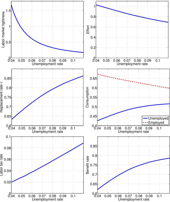
This section considers static equilibria where technologyat =aif fixed (no aggregate shocks) and analyzes how the equilibria vary with technology level a.17 Environments with lower technol-ogy have higher unemployment. Figure2displays in six panels, as a function of unemployment: (a) labor market tightness, (b) job-search effort, (c) optimal replacement rateτ=cu/ce, (d) opti-mal consumptions ce andcu, (e) optimal labor tax ratet =1−ce/w, and (f) optimal benefit rate
b=cu/w. Panels (a) is a Beveridge curve, showing that labor market tightness decreases with unemployment. Panel (b) shows that effort decreases with unemployment. Panel (c) displays the critical result of this section: the optimal replacement rate is strongly countercyclical, for it in-creases from 64% to 86% when unemployment inin-creases from 4% to 11%. The simulation in panel (c) confirms that the theoretical result of Proposition4also holds in our calibrated infinite-horizon model. It implies that consumption of unemployed workers increases relative to that of employed workers in recession. Panel (d) goes one step further: it shows that consumption of un-employed workers even increases in absolute terms. Panels (e) and (f) show that both benefit rate and labor tax rate should be countercyclical. In recession, labor tax should increase substantially, not only to finance benefits to a larger number of unemployed workers, but also to finance benefits that are more generous relative to the prevailing wage.
4.3
Formula in sufficient statistics
Figure2depicts the optimal replacement rateτ(a)as a function of the underlying technology level. To obtain such a scheduleτ(a), one needs to specify and calibrate the entire structure of the model. In this section, we present an alternative approach to determining optimal UI, which only requires estimating a few sufficient statistics that summarize the relevant characteristics of the model.
We assume that disutility of effort is isoelastic:k(e) =ωk·e1+κ/(1+κ). In the infinite-horizon
17In a static environment, the labor market is in steady state: the Beveridge curve (14) holds. In search-and-matching
models, the comparison of static environments delivers the same qualitative predictions as the study of a stochastic environment [Michaillat,forthcoming;Pissarides,2009].
0.040 0.05 0.06 0.07 0.08 0.09 0.1 0.5
1 1.5
Unemployment rate
Labor market tightness
0.040 0.05 0.06 0.07 0.08 0.09 0.1 0.2 0.4 0.6 0.8 1 Unemployment rate Effort 0.04 0.05 0.06 0.07 0.08 0.09 0.1 0.6 0.65 0.7 0.75 0.8 0.85 Unemployment rate Replacement rate τ 0.04 0.05 0.06 0.07 0.08 0.09 0.1 0.4 0.45 0.5 0.55 0.6 0.65 Unemployment rate Consumption Unemployed Employed 0.04 0.050 0.06 0.07 0.08 0.09 0.1 0.02 0.04 0.06 0.08 0.1 Unemployment rate
Labor tax rate
0.04 0.05 0.06 0.07 0.08 0.09 0.1 0.6 0.65 0.7 0.75 0.8 0.85 Unemployment rate Benefit rate
Figure 2: Optimal unemployment insurance over the business cycle
Notes:All computations are based on the infinite-horizon model calibrated in Table1. Each panel plots a collection of optimal equilibria in static environments characterized by different underlying technology levels: the unemployment rate uspans [0.04,0.11]for technologya∈[0.96,1.04]. The Appendix characterizes these optimal equilibria, and presents the numerical computations in detail.
0.040 0.05 0.06 0.07 0.08 0.09 0.1 0.1 0.2 0.3 0.4 0.5 Unemployment rate Elasticity of (1−n) wrt ∆ C Macro Micro 0.04 0.05 0.06 0.07 0.08 0.09 0.1 0.4 0.5 0.6 0.7 0.8 0.9 1 Unemployment rate Replacement rate τ Optimum Approximated formula Baily with macro−elasticity Baily with micro−elasticity
Figure 3: Micro-elasticity, macro-elasticity, and replacement rates
Notes: Both panels are based on the infinite-horizon model calibrated in Table1. The left panel plots, as a function of unemployment, the elasticities of unemployment 1−nwith respect to reward from work∆c=ce−cu, obtained for τ=65%. Macro-elasticityεM (blue, solid line) and micro-elasticityεm(red, dashed line) are defined and computed
in the Appendix. The right panel plots replacement rates as a function of unemployment. The red, dashed line is the replacement rate obtained with the Baily-Chetty formula using micro-elasticityεm: τ/(1−τ) = (ρ/εm)·(1−τ).
The magenta, dotted with circles, line is the replacement rate obtained with the Baily-Chetty formula using macro-elasticityεM: τ/(1−τ) = (ρ/εM)·(1−τ). The blue, solid line is the replacement rate obtained with formula (20).
For comparison, the green, dashed with circles, line is the exact optimal replacement rate plotted in Figure2. Each point corresponds to a different underlying technology levela:u∈[0.04,0.11]fora∈[0.96,1.04].
setting formula (10), obtained in the one-period model of Section2, becomes:18
τ 1−τ ≈ ρ εM·[1−τ] + 1+κ κ · εm εM −1 ·h1+ρ 2·(1−τ) i . (20)
This approximated formula is valid in a static environment ifn≈1,uκ,δ≈1, and the third and higher order terms ofv(·)are small. The termκ/(1+κ)in (10) is replaced by(1+κ)/κin (20), capturing an increase in the welfare cost of the rat-race externality in the infinite-horizon model, relative to the one-period model.19
The left panel in Figure 3 displays micro-elasticity εm and macro-elasticity εM of unemploy-ment with respect to net reward from work as a function of the unemployunemploy-ment rate for a constant replacement rate τ=65% (the average replacement rate in the US). The panel confirms that the 18The optimal UI formula (10) in the one-period environment is obtained without making any functional-form
assumption. The optimal search decision (17) is more complex in the infinite-horizon environment as it involves not onlyk0(e)as in the static model but also the levelk(e). Relatingk(e)tok0(e)requires the isoelasticity assumption.
results from Propositions2and3extend to this infinite-horizon environment: (1) macro-elasticity is always smaller than micro-elasticity and the wedge between the two elasticities increases in recessions; and (2) the macro-elasticity decreases in recessions. Furthermore, these cyclical fluc-tuations are quantitatively large: the ratioεm/εM increases from 5/4 when unemployment is 4% to 8 when unemployment is 11%; the macro-elasticity decreases from 0.40 when unemployment is 4% to 0.05 when unemployment is 11%. At the same time, the micro-elasticity remains broadly constant. It stays in the narrow 0.4–0.5 range when unemployment varies between 4% and 11%.
The right panel in Figure 3displays the replacement rate obtained from three alternative for-mulas, as a function of unemployment. This panel illustrates the discussion of the optimal UI formula presented in Section 2.6. The green dotted line plots the exact optimal replacement rate of Figure2. The blue solid curve is the replacement rate obtained with the approximated optimal UI formula (20). Those two curves are almost identical showing that formula (20) delivers an excellent approximation to the exact optimum. Next, the magenta dotted line is the replacement rate obtained from a Baily-Chetty formula, similar to (20) but excluding the term correcting for the rate-race externality. This replacement rate is lower than the full optimum because the correction term is positive as there is a positive wedge between micro- and macro-elasticity. Finally, the red dashed line is the replacement rate obtained from a standard Baily-Chetty formula, similar to (20) but excluding the correction term and replacing macro-elasticity εM by micro-elasticityεm in the first term. As micro-elasticity is almost acyclical, this replacement rate is almost acyclical as well: it varies within the narrow 48%–52% range. While this replacement rate, used in the public eco-nomics literature [for example,Gruber,1997], is close to the optimum when unemployment is low, it departs significantly from it in recession.20
4.4
The government can borrow and save
So far, we constrained the government to balance its budget each period. The government could not use deficit spending to shift resources intertemporally from expansions to recessions and smooth 20The micro-elasticity would be slightly more cyclical with higher risk aversion. A higher risk aversion would also
increase significantly the optimal replacement rate and would quantitatively reduce the difference in replacement rates between our formula and the standard Baily-Chetty formula.
−1% −0.5% 0% Technology No deficit spending Deficit spending 0% 2% 4% 6% Unemployment 0% 0.5% 1% Replacement rate τ 0% 0.5% 1% Deficit 0 50 100 150 200 250 300 −1% −0.5% 0% 0.5% 1% Consumption (employed)
Weeks after shock
0 50 100 150 200 250 300 −1% −0.5% 0% 0.5% 1% Consumption (unemployed)
Weeks after shock
Figure 4: Impulse response of optimal unemployment insurance to a negative technology shock
Notes:This figure displays impulse response functions (IRFs), which represent the percentage-deviation from steady state for each variable. We assume that the log-deviation of technology ˇat ≡dln(at) follows an AR(1) process:
ˇ
at+1=ν·aˇt+zt+1wherezt ∼N(0,σ2)is an innovation to technology. As inMichaillat[forthcoming], we estimate
this AR(1) process using BLS data for 1964:Q1–2010:Q2 and findν=0.991 andσ=0.0026 at weekly frequency. IRFs are obtained by imposing an unexpected negative technology shockz1=−0.01 to the log-linear infinite-horizon
model. The time period displayed on the x-axis is 300 weeks. The blue solid IRFs are responses of the optimal equilibrium when the government is constrained by (15) to balance its budget each period. The red dashed IRFs are responses of the optimal equilibrium when the government is subject to a single intertemporal budget constraint (21). Both log-linear systems and the IRFs computations are described in the Appendix.
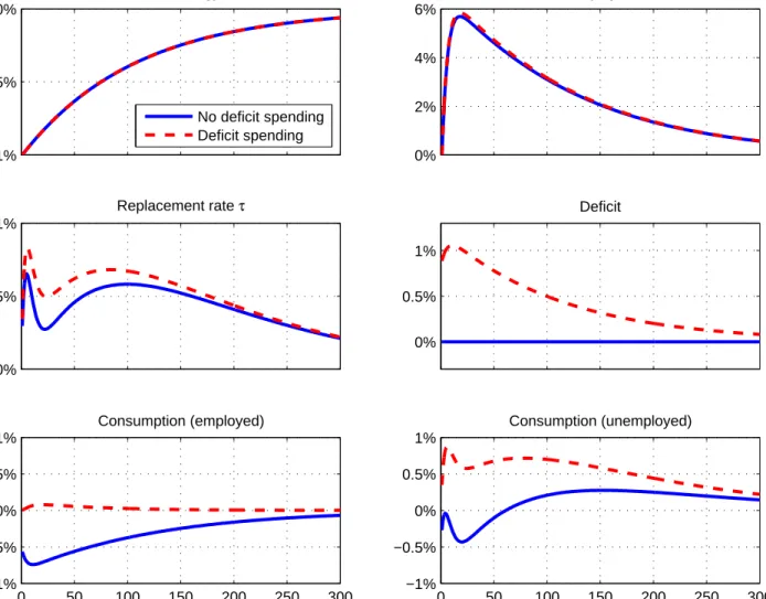
workers’ consumption. This modelling choice allowed us to focus on the trade-off between insur-ance and incentive to search within each period. However, it is important to understand how our results change when the government is able to borrow and save as is the case in practice.
In this section, we show that our results are robust to assuming that the government has access to a complete market for Arrow-Debreu securities. We assume that the government faces risk-neutral investors with discount factor δon the security market. An Arrow-Debreu security pays one unit of consumption good after history at. The price of this security is δt·p(at), where p(at) is the probability of historyat based on time-0 information. The government trades securities at time 0 to finance UI in all histories, and faces a unique intertemporal budget constraint:
0=E0
+∞
∑
t=0
δt·[nt·w(at)−nt·cet −(1−nt)·ctu]. (21)
We solve the government’s problem by log-linearization as described in the Appendix. To con-firm the comovements of technology with optimal UI in a stochastic environment, we compute impulse response functions. Figure4depicts the response of optimal UI to a negative technology shock in two cases: (1) the blue solid lines are responses in the baseline case in which the gov-ernment is constrained by (15) to balance his budget each period; and (2) the red dashed lines are responses when the government is subject to a single intertemporal budget constraint (21). The response of the optimal replacement rate to an adverse economic shock is almost identical whether the government uses deficit spending or not. On impact, the replacement rate increases by 0.5%; it then falls slightly, before building again for 100 weeks; at its peak, it increases by about 0.7% in both cases. While the generosity of UI is similar in both cases, consumption ofbothemployed and unemployed workers is higher when the government can borrow. In that case, the government smoothes consumption of employed workers almost perfectly. In contrast, the consumption of employed workers falls by about 0.7% on impact when the government must balance its budget each period. Indeed when the government is able to borrow, its budget deficit—defined as bene-fit outlays minus tax revenue in the period—increases by about 1% on impact, a consequence of the additional consumption smoothing provided to workers in recessions. Finally, unemployment
responds similarly in both cases: it builds slowly and peaks after about 20 weeks.
4.5
Unemployment benefits have finite duration
For simplicity, we assumed that unemployment benefits were available to all unemployed workers, independently of the length of their unemployment spell, and that the government adjusted the level of unemployment benefits over the business cycle. In practice, unemployment benefits have finite duration and governments often modulate the generosity of UI over the business cycle by adjusting the duration rather than the level of benefits.21 While we could not account for the duration of UI in a one-period model, we build on our infinite-horizon model to analyze quantitatively this option. In this section, we assume that the replacement rate of UI is fixed, that unemployment bene-fits have finite duration, and that the government can adjust the duration of UI over the business cycle. We confirm that the optimal duration of UI is countercyclical. For tractability, we follow Fredriksson and Holmlund[2001] and assume that workers exhaust their unemployment benefits with probabilityλt at the end of each periodt. Eligible unemployed workers receive consumption cut from unemployment benefits, and ineligible unemployed workers receive consumptioncat <ctu
from social assistance until they find a job. At the beginning of period t, there are xtu jobseek-ers exerting job-search effort etu, and xat ineligible jobseekers exerting job-search effort eta. The matching process is the same as in the baseline model of Section4.1, except that we redefine labor market tightnessθt ≡ot/(eta·xat +eut ·xtu). After the matching,zut eligible jobseekers andzat
ineli-gible jobseekers are still unemployed. The stocks of workers are linked by the following relations:
zut =xtu·(1−eut ·f(θt)),zat =xta·(1−eat ·f(θt)),nt =1−(zat +ztu),xtu=ztu−1·(1−λt−1) +s·nt−1,
xat =zta−1+λt−1·zut−1. Worker’s and firm’s problems are very similar to those in Section 4.1,
and are described in the Appendix. We assume that the generosity of unemployment benefits: τu,e =cut/cte, as well as the generosity of social assistance: τa,e=cta/cet, are constant over time. The government chooses the rateλt at which eligible unemployed workers become ineligible, in
21US unemployment benefits have a maximum duration of 26 weeks in normal times. Duration is automatically
extended by up to 20 weeks in states where unemployment is above 8%. Duration is often further extended by the government in severe recessions. For example, the federal Emergency Unemployment Compensation program, enacted in 2008, extends durations by an additional 53 weeks when state unemployment is above 8.5%.
order to maximize social welfare E0 +∞
∑
t=0 δt·[−xut ·k(etu)−xat ·k(eta) +nt·v(cte) +zut ·v(ctu) +zat ·v(cat)],su