OpenBU http://open.bu.edu
Theses & Dissertations Boston University Theses & Dissertations
2015
Optimization methods for
side-chain positioning and
macromolecular docking
https://hdl.handle.net/2144/16091COLLEGE OF ENGINEERING
Dissertation
OPTIMIZATION METHODS FOR SIDE-CHAIN
POSITIONING AND MACROMOLECULAR DOCKING
by
MOHAMMAD MOGHADASI
B.S., Sharif University of Technology, Tehran, Iran 2009
Submitted in partial fulfillment of the
requirements for the degree of
Doctor of Philosophy
2015
MOHAMMAD MOGHADASI
All rights reserved
First Reader
Ioannis Ch. Paschalidis, PhD
Professor of Electrical and Computer Engineering Professor of Systems Engineering
Professor of Biomedical Engineering
Second Reader
Pirooz Vakili, PhD
Associate Professor of Mechanical Engineering Associate Professor of Systems Engineering
Third Reader
Sandor Vajda, PhD
Professor of Biomedical Engineering Professor of Chemistry
Fourth Reader
Dima Kozakov, PhD
Research Associate Professor of Biomedical Engineering
Fifth Reader
Bobak Nazer, PhD
Assistant Professor of Electrical and Computer Engineering Assistant Professor of Systems Engineering
love and steadfast support and encouragement throughout my studies. To my best friend, Ali Khodabakhsh, who left us so early.
First and foremost, I would like to express the deepest appreciation to my PhD advisor Professor Ioannis Paschalidis for his support, encouragement and counsel over the past five years. Working with him has been a tremendously rewarding experience, helping me grow professionally and individually along the way. His enlightening mentorship along with his wide knowledge have provided invaluable insights in how to conduct research projects and work as a part of a team. I am deeply grateful for having the privilege of being supervised by Professor Paschalidis and learning so much from him. I would also like to thank Professor Pirooz Vakili, Professor Sandor Vajda, Profes-sor Bobak Nazer and Dr. Dima Kozakov for serving as my committee members and also their guidance and comments during the course of my PhD, that have greatly enriched the work. I am sincerely grateful to them for generously sharing their knowl-edge and illuminating views on various aspects of this dissertation. Without their guidance and constant help this dissertation would not have been possible. I also want to thank to Professor James Perkins for his time and consideration to serve as the chair of my defense session.
In addition, I thank the head of Systems Engineering division, Professor Christos Cassandras, for giving me support and mentorship during Summer 2010 in which I worked in his group. I would also like to show my gratitude to all the administrative staff of Systems Engineering division, in particular, Ms. Elizabeth Flagg. I am truly grateful to my former and current collaborators both in Network Optimization and Control lab and Structural Bioinformatics lab.
I would like to take this opportunity to thank all my dear friends who have been for me a family and leave me so many unforgettable memories during my stay in Boston: Setareh Ariafar, Mohammad Reza Aghajani, Asieh Ahani, Ramtin Arian, Mohammad Hossein Asgari, Armin Ataei, Amir Banari, Saber Bohrani, Morteza
Shima Koohakipour, Hanieh Mirzaei, Delaram Motamed Vaziri, Ali Nejat, Amirreza Oghbaee, Sepideh Pour Azaram, Mina Yaghmazadeh, Kiana Yazdifar, and many others.
Last but not least, a special thanks to my family for their unconditional love and priceless support and encouragement throughout the duration of my studies. I can not express in words, my deepest gratitude for my parents, Beitolah and Maryam, for everything they have given to me and for their incredible patience and sacrifice during my graduate studies. I also want to thank my lovely sister, Soodeh, for encouraging me constantly to complete this work, and my dear brother, Meisam, for solidly standing behind me in my ups and downs all these years. Thanks to them both for being an immense source of inspiration throughout my life. Moreover, I am thankful to my little brother, Ali, for believing in me and being a great source of joy, happiness and motivation. Finally, I would like to thank my sister-in-law, Sahar, for all her invaluable care and kindness toward me.
POSITIONING AND MACROMOLECULAR DOCKING
MOHAMMAD MOGHADASI
Boston University, College of Engineering, 2015
Major Professor: Ioannis Ch. Paschalidis, PhD,
Professor of Electrical and Computer Engineering,
Professor of Systems Engineering,
Professor of Biomedical Engineering
ABSTRACT
This dissertation proposes new optimization algorithms targeting protein-protein docking which is an important class of problems in computational structural biology. The ultimate goal of docking methods is to predict the 3-dimensional structure of a stable protein-protein complex. We study two specific problems encountered in predictive docking of proteins. The first problem is Side-Chain Positioning (SCP), a central component of homology modeling and computational protein docking meth-ods. We formulate SCP as a Maximum Weighted Independent Set (MWIS) problem on an appropriately constructed graph. Our formulation also considers the significant special structure of proteins that SCP exhibits for docking. We develop an approxi-mate algorithm that solves a relaxation of MWIS and employ randomized estimation heuristics to obtain high-quality feasible solutions to the problem. The algorithm is fully distributed and can be implemented on multi-processor architectures. Our com-putational results on a benchmark set of protein complexes show that the accuracy of our approximate MWIS-based algorithm predictions is comparable with the results achieved by a state-of-the-art method that finds an exact solution to SCP.
propose two different methods to solve the refinement problem. The first approach is based on a Monte Carlo-Minimization (MCM) search to optimize rigid-body and side-chain conformations for binding. In particular, we study the impact of opti-mally positioning the side-chains in the interface region between two proteins in the process of binding. We report computational results showing that incorporating side-chain flexibility in docking provides substantial improvement in the quality of docked predictions compared to the rigid-body approaches. Further, we demonstrate that the inclusion of unbound side-chain conformers in the side-chain search introduces significant improvement in the performance of the docking refinement protocols. In the second approach, we propose a novel stochastic optimization algorithm based on Subspace Semi-Definite programming-based Underestimation (SSDU), which aims to solve protein docking and protein structure prediction. SSDU is based on un-derestimating the binding energy function in a permissive subspace of the space of rigid-body motions. We apply Principal Component Analysis (PCA) to determine the permissive subspace and reduce the dimensionality of the conformational search space. We consider the general class of convex polynomial underestimators, and formulate the problem of finding such underestimators as a Semi-Definite Program-ming (SDP) problem. Using these underestimators, we perform a biased sampling in the vicinity of the conformational regions where the energy function is at its global minimum. Moreover, we develop an exploration procedure based on density-based clustering to detect the near-native regions even when there are many local minima residing far from each other. We also incorporate a Model Selection procedure into SSDU to pick a predictive conformation. Testing our algorithm over a benchmark of protein complexes indicates that SSDU substantially improves the quality of docking refinement compared with existing methods.
1 Introduction 1
1.1 Protein structure . . . 1
1.2 Protein docking problem . . . 3
1.3 Side-chain positioning problem . . . 5
1.4 MWIS algorithm for side-chain positioning . . . 6
1.4.1 Maximum weighted independent set problem; edge-constrained 6 1.4.2 Maximum weighted independent set problem; clique-constrained 7 1.4.3 SCP as an MWIS problem . . . 8
1.5 PIPER: sampling docked receptor-ligand conformations . . . 9
1.6 Monte Carlo-minimization approach for docking . . . 10
1.7 SSDU: a global optimization algorithm for docking . . . 12
1.8 Thesis contribution . . . 12
1.8.1 MWIS-based algorithms for SCP problem . . . 12
1.8.2 MCM algorithm for protein docking . . . 13
1.8.3 Studying the impact of SCP in docking methods . . . 13
1.8.4 SSDU algorithm for protein docking . . . 14
1.9 Thesis outline . . . 15
2 Edge-constrained MWIS algorithm for side-chain positioning 16 2.1 Side-chain positioning problem . . . 16
2.2 Related work . . . 17
2.3 Quadratic integer programming formulation . . . 20
2.5 Our distributed algorithm for edge-constrained MWIS . . . 24
2.5.1 Phase 1a: coloring . . . 25
2.5.2 Phase 1b: gradient projection . . . 27
2.5.3 Phase 2: estimation . . . 30
3 Clique-constrained MWIS algorithm for side-chain positioning 33 3.1 The MWIS formulation: clique-constrained . . . 33
3.2 Our distributed algorithm for clique-constrained MWIS . . . 34
3.2.1 Phase 1: gradient projection . . . 34
3.2.2 Phase 2: estimation . . . 37
3.3 Optimality for perfect graphs . . . 39
3.4 Solving SCP as a clique-constrained MWIS . . . 40
3.4.1 An exact algorithm for 2-residue clusters . . . 41
3.4.2 An approximate algorithm for 2-residue clusters . . . 43
3.4.3 An approximate algorithm for larger clusters . . . 44
4 MWIS application in side-chain prediction 45 4.1 Implementation choices of MWIS . . . 45
4.1.1 Accuracy vs. runtime trade-off . . . 45
4.1.2 Inclusion of unbound conformers . . . 46
4.1.3 Comparing MWIS with SCWRL4 . . . 46
4.2 Rotamer Selection . . . 47
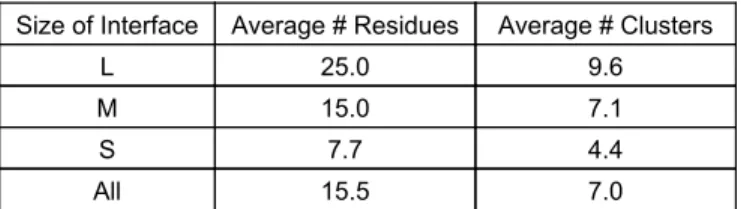
4.3 Partitioning the interface residues . . . 49
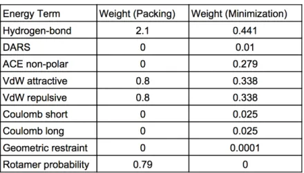
4.4 Energy Function . . . 51
4.5 Edge-constrained vs. Clique-constrained MWIS . . . 52
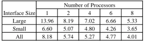
4.6 Effect of Parallelization on Running Time . . . 54
4.7 Results and Discussion . . . 56
5.1 FFT-based docking . . . 60
5.2 Global docking using the clusPro server . . . 63
5.3 Focused resampling of the near-native region . . . 65
5.4 MCM-based off-grid refinement . . . 66
5.5 Benchmark set of complexes for protein docking . . . 68
5.6 Results and discussion . . . 70
6 The impact of SCP on protein docking refinement 77 6.1 Off-grid minimization with an optional SCP step . . . 77
6.2 Inclusion of unbound conformers . . . 78
6.3 Refinement set generation . . . 79
6.4 Results and discussion . . . 80
7 The SSDU algorithm for protein docking refinement 85 7.1 SSDU overview . . . 85
7.2 Related work . . . 86
7.3 Contributions of SSDU . . . 87
7.3.1 Dimensionality Reduction . . . 87
7.3.2 General Class of Convex Underestimators . . . 88
7.3.3 Clustering and Model Selection . . . 88
7.4 Dimensionality Reduction . . . 89
7.5 Underestimation . . . 92
7.6 Sampling . . . 95
7.7 Clustering and Outlier Elimination . . . 96
7.8 SSDU Algorithm . . . 98
7.9 Post-Processing Model Selection . . . 100
7.10 Local Minimization . . . 102
7.11.1 Energy Function . . . 103
7.11.2 Refinement dataset . . . 105
7.12 Results and Discussions . . . 106
7.12.1 Protein Docking Refinement . . . 107
7.12.2 Model Selection . . . 110
7.12.3 The Impact of PCA and Clustering . . . 112
8 Conclusions and future directions 119 8.1 Future Research Directions . . . 121
8.1.1 Improving the accuracy of MWIS algorithm . . . 121
8.1.2 Monte Carlo minimization in permissive subspace . . . 122
8.1.3 PIPER Cluster discrimination using SSDU . . . 123
A Proofs 124 A.1 Proofs of Chapter 2 . . . 124
A.2 Proofs of Chapter 3 . . . 128
A.3 Proof of Chapter 7 . . . 131
References 132
Curriculum Vitae 140
4.1 Analysis on the number of clusters of the interface residue set. . . . 51 4.2 The weights of each term of the scoring function used at different steps
of the optimization procedure. The column labeled packing shows the weights for the side-chain packing step, and the column labeled mini-mizationlists the weights for the rigid-body minimization step. . . 53 4.3 The actual running time of the SCP algorithm for different number
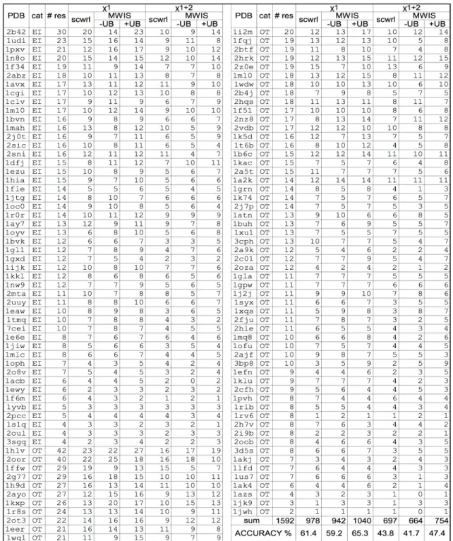
of processors. The first column refers to the category of the proteins based on the size of their interface set. For each category, the average running time values over the ensemble of proteins which belong to that category are reported in columns 2-6. The numbers in the second row indicate the number of processors that has been used for different settings. . . 57 4.4 Comparing SCWRL4.0 and MWIS to native. We compare the
per-formance of SCP of 3 modes: scwrl shows the prediction accuracy of SCWRL4.0,MWIS−UBandMWIS +UBdenote the performance of our MWIS algorithm without and with considering the unbound conformers respectively. Moreover, we report the number of the in-terface residues whose predicted conformation is considered accurate based on theχ1 and χ1+2 criteria. . . 59
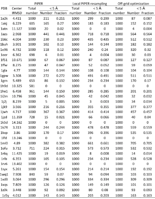
native complex at different stages of the refinement. . . 72 5.2 Figure 5.1 cont’d – The number of docking decoys within the 5˚A
IRMSD neighborhood of native complex at different stages of the re-finement. . . 73
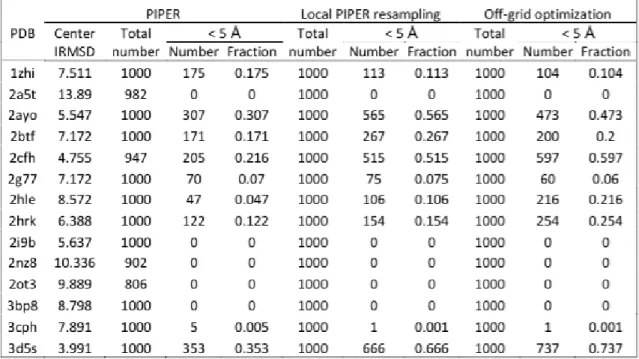
6.1 We compare three different refinement modes of a refinement algorithm to demonstrate: (i) the effect of side-chain packing on docking refine-ment, and (ii) the importance of including the unbound conformers. In each case, we report the number of near-native structures (within 5 ˚A RMSD from the native) amongst the refinement set of size 1,000. In the table,R-SPstands for refinement without SCP,R+SP-UBdenotes refinement with SCP but without unbound conformers andR+SP+UB
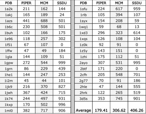
denotes refinement with SCP and with unbound conformers). . . 82 7.1 Comparing refinement results of MCM and SSDU methods over a
benchmark of 34 OT protein complexes. PDB column lists the PDB codes of the proteins,PIPERcolumn reports the number of near-native hits in the initial conformation set of each complex, and MCM and
SSDUcolumns include the number of near-native predicted conforma-tions using these two different refinement methods. . . 107
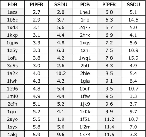
PIPER cluster center and the SSDU selected model. The PDB col-umn lists the PDB codes of the proteins (the proteins are sorted by the RMSD value of the PIPER cluster center). The PIPER column indicates the RMSD of the PIPER cluster center to the native struc-ture and the SSDU column reports the RMSD of the selected model by SSDU to the native.. . . 112
1·1 3-D representation of an actual protein-protein interaction. The pep-tide in red is the receptor, and the one in blue is the ligand protein.
. . . 2 1·2 A peptide composed of 4 residues separated by dashed lines. Each
residue is composed of two elements: the side-chain of each residue i is specified by Ri, and the other atoms form the backbone part of the residue. N terminus and C terminus are the start and the end of the peptide chain. (Source: http://www.molecularstation.com) . . . 2 1·3 Schematic of a peptide backbone composed of tens of residues (Source:
http://quantum-mind.co.uk/). . . 3 1·4 Protein docking aims to find the native conformations of protein-protein
interactions by minimizing the free energy of the complex. (Source: http://www.lpds.sztaki.hu/) . . . 4
1·5 Protein docking attempts to find the global minimum of the binding energy function in order to determine the structure of a complex in atomic detail. . . 5 1·6 SCP resolves the steric clashes in the interface of protein 1DFJ. . . . 7
CMBI) . . . 17
2·2 The |I|-partite graph used to derive the QIP formulation (2.2). The red nodes and edge indicate that rotamerirfrom residueiand rotamer js from residue j were selected. The weight of each edge of the graph represents the interaction energy between the associated rotamer pair. 22 2·3 Construction of the graphical model of a system with 2 residuesi and j with sets of rotamers: Ui ={ir1, ir2, ir3}and Uj ={js1, js2}. The op-timal set of rotamers of the residuesiandj can be obtained by finding the MWIS of this weighted graph. Let the triple {ir1ir1, ir1js2, js2js2} be the MWIS, then the solution to the SCP problem will be rotamers ir1 and js2 for residues i and j, respectively. . . 24
2·4 Competition algorithm to find the root. . . 26
2·5 Gradient projection algorithm for solving (3.4). . . 29
2·6 Rounding x∗ to obtain a feasible solution for (2.3). . . 31
3·1 Gradient projection algorithm for solving (3.4). . . 36
3·2 Greedy estimation algorithm to obtain a feasible solution to the MWIS problem (3.1). . . 38
4·1 Generating rotamers by changing χ1 angle. . . 48
residues are colored with yellow, and the rest of receptor and lig-and resides are colored with blue lig-and green respectively. (Source: http://www.stats.ox.ac.uk/ hamer/research.html) . . . 49
4·3 The speedup wrt the single-processor run for 2-, 4-, 6- and 8-processor settings. The vertical axis shows the speedup value, and the horizontal axis depicts the number of processors. Different categories of protein ensembles (Large, Small and All) are plotted. . . 56
5·1 Representation of local translation and rotation grids employed by the PIPER resampling. A) translation; B) rotation. The receptor molecule, shown in red, is fixed. Ligand orientations correspond to different grid points and are shown in different colors. Initial ligand orientation that defines the center of the cluster was taken from global PIPER docking simulation. For clarity of the picture only 20 rotations out of 3200 are shown for this complex. Note that only relatively small rotations are employed in our local resampling procedure. . . 67 5·2 MCM-based off-grid refinement iteratively applies rigid-body
minimiza-tion and SCP to protein conformaminimiza-tions. . . 68 5·3 Fraction of docked structures with less than 5˚A IRMSD among the
structures generated by ClusPro (blue triangles) and by focused re-sampling of the near-native cluster obtained by the global docking (red squares). Results are shown for the 49 complexes listed in Table 5.1. 69
structures of four different complexes. For each complex, IRMSD dis-tributions are shown for the results from the global docking using PIPER (black curve); after resampling the most near-native cluster of PIPER generated structures (red curve); and after off- grid refine-ment by five steps of the MCM algorithm over the structures from the focused resampling (green curve). A) Complex of the cytoplasmic do-main of the type I TGF receptor and and FKBP12, PDB ID:1B6C; B) Human PPARγ and RXRα ligand binding domains PDB ID: 1K74; C) Adenylyl cyclase in a complex with its stimulatory heterotrimeric G protein alpha subunit, PDB ID: 1AZS; and D) Disulfide-linked com-plex between the N- terminal domain of the electron transfer catalyst DsbD and the cytochrome c biogenesis protein CcmG, PDB ID: 1Z5Y. 75
6·1 The effect of different modes of docking on increasing/decreasing the accuracy of PIPER outputs for the EI benchmark. The values on the vertical axis denote the number of additional accurate conformations wrt PIPER that each refinement mode predicts. The horizontal axis shows the PDB codes of each protein complex. For each mode, these discrete data points are fit to a curve to illustrate the overall perfor-mance of each case. . . 83 6·2 The effect of different modes of docking on increasing/decreasing the
accuracy of PIPER outputs for the OT benchmark. The plots have the same specifications as captioned in Figure 6·1. . . 84
polynomial. (Source: (Shen et al., 2008)). . . 92 7·2 Illustration of how clustering resolves a difficult case with multiple local
minima residing far from each other. Using a single underestimator for this case, the minimum of the underestimator may lie in a region far from the global minimum of the binding energy function. . . 97
7·3 The flowchart of the SSDU procedure. . . 98 7·4 SSDU iterations over the protein complex 1grn. The x-axis shows
the RMSD-to-native of the conformations in ˚A, and the y-axis shows the interaction energy between the receptor and ligand. The number of hits written above the plots indicates the number of near-native conformations for each iteration. . . 100 7·5 The flowchart of the MCM-based off-grid refinement procedure. . . . 104 7·6 The performance of SSDU in improving the PIPER conformations.
The x-axis includes 34 protein complexes of the benchmark sorted by the number of PIPER near-native hits, and the y-axis shows the num-ber of near-native conformations out of an ensemble of 1000 conforma-tions. . . 108
tioning the benchmark set into two groups of protein complexes based on the number of near-native input conformations. Thex-axis includes these two different ranges of input protein systems, and the y-axis in-dicates the average number of near-native predictions over each range.
. . . 109 7·8 Comparing the distribution of model RMSD-to-native of PIPER and
SSDU over the benchmark. The x-axis consists of 6 different ranges for RMSD values with a bin size of 2˚A, and the y-axis indicates the population of each range. . . 111 7·9 The effect of clustering and outlier elimination on the performance
of SSDU algorithm. Each column of plots shows the results for one protein complex. Protein complexes with PDB ID’s 1buh, 1jk9 and
1ml0 are shown in columns 1−3 respectively. The rows 1−3 shows the ensemble of conformations ofPIPER,SSDU without clusteringand
SSDU with clustering respectively. The x-axis shows the RMSD-to-native of the conformations in ˚A, and the y-axis shows the interaction energy between the receptor and ligand. . . 113 7·10 System-based Comparison of SSDU Modes. . . 115 7·11 Comparing 4 different modes of SSDU algorithm using a transitional
graph . . . 118
3-D . . . 3-Dimensional
ACE . . . Analytical Continuum Electrostatic
CAPRI . . . Critical Assessment of PRotein Interactions CGU . . . Convex Global Underestimator
DARS . . . Decoys as Reference State
DBSCAN . . . Density-Based Spatial Clustering of Applications . . . with Noise
DEE . . . Dead-End Elimination EI . . . Enzyme-Inhibitor FFT . . . Fast Fourier Transform GP . . . Gradient Projection
ILP . . . Integer Linear Programming IP . . . Integer Programming
IRMSD . . . Interface Root Mean Square Deviation LP . . . Linear Programming
NP-hard . . . Non-deterministic Polynomial-time hard OT . . . Others
PCA . . . Principal Component Analysis PDF . . . Probability Distribution Function QIP . . . Quadratic Integer Programming RMSD . . . Root Mean Squared Deviation SCP . . . Side-Chain Positioning
SDP . . . Semi-Definite Programming SE(3) . . . Special Euclidean group SGS . . . Semi-Global Simplex
SOCP . . . Second Order Cone Programming SDU . . . Semi-Definite programming-based
. . . Underestimation SOS . . . Sum-Of-Square wrt . . . with respect to
Chapter 1
Introduction
1.1
Protein structure
Proteins are one of the key elements of the cell. Proteins are very large biological molecules, or macromolecules, which interact with each other or with other chemical entities to perform a particular cellular function. These interactions form a stable protein complex and play a central role in a number of cellular functions such as cell signaling, metabolic control and gene regulation. At each protein interaction, at least two chemical compounds are involved: a receptor which is the larger protein molecule to which other molecules can bind, and a ligandthat is a relatively smaller molecule binding to the receptor. In Figure 1·1, a 3-dimensional (3-D) representation of an actual protein-protein interaction is shown, in which the ligand is binding to the receptor.
Each protein molecule consists of one or more compounds calledpeptides. Peptides are a sequence of unbranched chains of recurring elements calledamino acid residues. The number of residues linked in a peptide can be as few as two, or perhaps as many as hundreds. Each residue is a small molecule composed of two groups of atoms, backbone and side-chain. The structure of the backbone part is the same for all residues composed of amine (−N H2) and carboxylic acid (−COOH) functional groups. However, the side-chain structure may differ from one residue to another. Natural amino acids are usually classified by the molecular structure of their side-chain into 21 different types. The side-side-chain of each residue has one end attached to
Figure 1·1: 3-D representation of an actual protein-protein interaction. The peptide in red is the receptor, and the one in blue is the ligand protein.
the backbone and another unattached end which can freely move in space. Residues of the same chain are linked together via their backbone groups, and the sequence of all backbone groups in a chain is called the backbone. Figure 1·2 shows a simple peptide including 4 residues separated by dashed lines.
Figure 1·2: A peptide composed of 4 residues separated by dashed lines. Each residue is composed of two elements: the side-chain of each residueiis specified byRi, and the other atoms form the backbone part of the residue. N terminus and C terminus are the start and the end of the peptide chain. (Source: http://www.molecularstation.com)
In general, most of the protein peptides have so many chained residues. Figure 1·3 shows the backbone of such a peptide which is composed of tens of residues.
Figure 1·3: Schematic of a peptide backbone composed of tens of residues (Source: http://quantum-mind.co.uk/).
1.2
Protein docking problem
Protein dockingis the problem of predicting the tertiary structure of a stable receptor-ligand complex (Halperin et al., 2002), (Smith and Sternberg, 2002). Based on the principles of thermodynamics, when a number of chemical compounds, including proteins, bind to each other, the most stable state of the system (thenativestructure) occurs when the Gibbs free energy of the complex attains its minimum value. To get to this native state of the bound complex, the backbones and the side-chains of the unbound state of these macromolecular entities move to take a new conformation which has the lowest energy.
In this light, the protein docking problem is an optimization problem in which the variables are the atomic coordinate of the proteins and the objective is to minimize the energy of the complex that is a function of all those variables. However, solving such a problem with so many variables would be computationally infeasible, and some simplification is needed. Figure 1·4 depicts the process of docking for a receptor-ligand complex. There are three options shown in this figure as the possible docked conformations, but docking picks the one with the lowest interaction energy value.
Figure 1·4: Protein docking aims to find the native conformations of protein-protein interactions by minimizing the free energy of the complex. (Source: http://www.lpds.sztaki.hu/)
The protein docking problem has attracted significant attention during the last few decades and many computational approaches have attempted to solve it. In spite of this, docking is still regarded as a very challenging problem in structural biology due to the complexity of the energy landscape of protein-protein interactions.
This complexity comes from the fact that the energy function is composed of mul-tiple force-field energy terms (such as Lennard-Jones potential, solvation, knowledge-based hydrogen bonding, coulomb potential, statistical energy, etc.) with different space scales resulting in a multi-frequency behavior of the high-frequency terms. Therefore, the energy function in hand has multiple deep funnels and extremely many local minima over its multidimensional domain (Moghadasi et al., 2015b). Figure 1·5 illustrates the simplified schematics of the binding energy function with a 2-D
confor-mational space (for rigid-body docking the conforconfor-mational space has 6 dimensions).
Figure 1·5: Protein docking attempts to find the global minimum of the binding energy function in order to determine the structure of a complex in atomic detail.
1.3
Side-chain positioning problem
Side-chain positioning (SCP) is one of the key components of protein docking meth-ods, and is extremely important in the context of protein-protein association. As the two partner proteins approach each other, side-chains in the interface region between the proteins tend to re-orient so as to avoid steric clashes and facilitate the process of binding. Capturing this effect algorithmically has the potential to enhance docking protocols (Moghadasi et al., 2015a).
SCP enables the rigid-body docking algorithms to take advantage of the flexibility of the protein side-chains in order to predict the lowest energy conformation. In general, side-chains are more flexible than the backbone, and positioning them is a critical component of protein structure prediction (Lee and Subbiah, 1991), (Summers and Karplus, 1989), (Holm and Sander, 1991). When a ligand binds to a receptor, considerable plasticity and conformational changes of the backbone and the
side-chains are often observed at the interfacial residues. These changes are of the form of slight displacements of the atoms at the interfacial regions of the receptor and ligand that overally decrease the energy of the complex. Ideally, one would like to predict the lowest energy conformation of the receptor and ligand backbones and side-chains. However, due to the high complexity of modeling the backbone movement and its typically rigid structure, most of the classical models keep the backbone fixed, while allowing the side-chains to freely move in space (Chazelle et al., 2004), (Kingsford et al., 2005). Thus, SCP can be defined as a problem which takes fixed receptor and ligand backbones and predicts the side-chain conformations that minimize the overall energy of the complex.
In Figure 1·6, an instance of SCP problem and its solution are shown. In this figure, the interface chains of the protein 1DFJ is depicted. The interface side-chains of the receptor and the ligand are respectively colored with red and green. The non-interface side-chains of the receptor and ligand are shown in gray and cyan respectively. The left plot shows that several steric clashes are observed in the inter-face which means the interaction energy of the complex is very high. If we solve SCP over this problem, the solution would be the interface shown on the right, meaning that the steric clashes are resolved and the energy of the complex is decreased.
1.4
MWIS algorithm for side-chain positioning
1.4.1 Maximum weighted independent set problem; edge-constrained
Maximum Weighted Independent Set (MWIS) is a well-studied Non-deterministic Polynomial-time hard (NP-hard) combinatorial optimization problem. The goal of the problem is to find the heaviest independent set of nodes in a given undirected graph G = (V,E) with non-negative weights on the nodes. A set is called indepen-dent if no two nodes in it are adjacent. We can formulate MWIS as the following
7
1DFJ interface before side-chain packing
• several steric clashes are observed
red interface side-chains of receptor green interface side-chains of ligand gray non-interface side-chains of receptor cyan non-interface side-chains of ligand (backbones are not shown)
Graphical model of side-chain packing problem based on integer-linear programming formulation
1DFJ interface after side-chain packing
• the steric clashes are resolved
Formulation
Distributed Optimization
Solution Problem1DFJ interface before side-chain packing
• several steric clashes are observed
red interface side-chains of receptor green interface side-chains of ligand gray non-interface side-chains of receptor cyan non-interface side-chains of ligand (backbones are not shown)
1DFJ interface after side-chain packing
• the steric clashes are resolved
Formulation
Distributed Optimization
Solution
Figure 1·6: SCP resolves the steric clashes in the interface of protein 1DFJ.
Integer Programming (IP) problem:
max PNi=1wixi
s.t. xi+xj ≤1, ∀(i, j)∈ E, xi ∈ {0,1}, i= 1, . . . , N,
(1.1)
where N = |V|, wi ≥ 0 is the weight of node i, and xi is the indicator variable of selecting node i. The cost function of (1.1) is the total weight of the selected nodes, and the inequality constraint ensures the independence of the selected set of nodes.
1.4.2 Maximum weighted independent set problem; clique-constrained
Our algorithm is an approximate approach based on solving theLinear Programming-relaxation (LP-Programming-relaxation) of the MWIS problem. Solving a tighter relaxation of MWIS allows us to approach more closely to the optimal MWIS solution. In this regards, in addition to the basic formulation of MWIS (1.1), we also consider an alternative formulation for the MWIS problem which involves more inequality con-straints enforced on the cliques of MWIS graphG. Given a graphG = (V,E), aclique
is a subset of nodes such that every two of them are adjacent. The maximum size of a clique in G is called the clique number of G. A maximal clique C is a clique of
G which cannot be extended by adding one more node. Let S ={C1,C2, . . .} denote the set of all maximal cliques of G. MWIS can be formulated as the Integer Linear Programming (ILP) problem:
max PNi=1wixi s.t. P i∈Cjxi ≤1, ∀j :Cj ∈ S, xi ∈ {0,1}, i= 1, . . . , N. (1.2) 1.4.3 SCP as an MWIS problem
We formulate SCP as a MWIS problem and devise distributed algorithms (Moghadasi et al., 2012), (Moghadasi et al., 2013) to solve it. We have developed two MWIS for-mulations to solve SCP problem which have slightly different set of constraints. The first formulation considers the edge-constrained MWIS (1.1), and the other one for-mulates SCP as a clique-constrained MWIS (1.2). The clique-constrained formulation of MWIS is an extension of the edge-constrained. In Section 4.5, we compare these algorithms and explain why the clique-constrained one is generally a more practical algorithm. Although the ILPs (1.1) and (1.2) describe the same feasible set, the LP-relaxation of (1.2) is tighter than that of (1.1). We will call the LP-LP-relaxation of (1.2) the clique relaxation of the MWIS. We will see how we can use a tighter relaxation to approach more closely an optimal MWIS solution.
Compared to alternative algorithms, the main advantage of our approach is that it uses distributed computations when solving the optimization problem, hence the algorithms can be efficiently implemented in a network of processors and involve only local communications between neighboring processors.
problem instances. Computational results on a protein docking benchmark set suggest that these solutions lead to high-accuracy side-chain predictions. The distributed nature of the algorithm can lead to fast solutions for large interfaces. In the context of SCP application, the parallel approach is very helpful due to the large problem instances one has to tackle.
Our SCP algorithm can be applied in two important contexts. First, we can use SCP as a general side-chain prediction method with applications in various areas of structural biology (see Chapter 4). Second, we incorporate SCP as a key element of protein docking procedure. We demonstrate that adding SCP to protein docking protocols significantly improves the docking performance (see Chapter 6).
1.5
PIPER: sampling docked receptor-ligand conformations
Our protein docking algorithm consists of multiple stages beginning with sampling an enormous number of docked receptor-ligand conformations with a rigid-body global search that uses theFast Fourier Transform (FFT)correlation approach. To conduct this initial sampling, we use ClusPro 2.0 that is based on a docking program called
PIPER (Kozakov et al., 2006). These conformations are then sorted by their free energy values, and the top several thousands ones with lowest energy values are retained for further processing. We cluster this set of low-energy conformations using the pairwise Root Mean Squared Deviation (RMSD) criterion which can be regarded as a distance measure (Kozakov et al., 2005). For each cluster, we find the cluster center as the conformation with the largest number of neighbors (two conformations are neighbors if their pair-wise RMSD is within a certain threshold). As a side story, the radius of the PIPER clusters can be used to improve the discrimination of near-native complex structures (Kozakov et al., 2005). In this work, however, our focus is mostly on protein docking refinement stage, and for this purpose, we only
consider the near-native clusters, i.e., the clusters whose cluster center is within an RMSD threshold to the native structure. For each near-native cluster, we sort all the cluster conformations by the RMSD value to the cluster center and pick the top conformations using an RMSD threshold of 12 ˚A.
The goal of protein docking refinement is to locate the global energy minimum within the regions of the conformational space. Following the procedure discussed above, the input to our refinement stage is an ensemble of the receptor-ligand con-formations sampled from certain PIPER clusters. The refinement protocol takes an initial set of sampled conformations as the input and aims to improve the quality of the set. One way to evaluate the performance of a refinement algorithm is to count the number of near-native output conformations it predicts compared to the initial input structures. The other criterion is based on the RMSD to native of the single selected model algorithm predicts, which is usually the cluster center of the confor-mation set. The ultimate goal is to increase the number of near-native predictions and to decrease the RMSD to native of the selected model.
We have developed two protein docking refinement algorithms which aim to refine the top conformations retained from the aforementioned sampling procedure. The first approach is based on Monte Carlo Minimization (MCM) (Moghadasi et al., 2015a), (Mamonov et al., 2015), and the second one is the Subsapce Semi-Definite programming based Underestimation (SSDU) (Moghadasi et al., 2015b), (Nan et al., 2014). In the sequel, we briefly introduce these methods.
1.6
Monte Carlo-minimization approach for docking
We propose a refinement algorithm based on an MCM approach which takes the ensemble of filtered conformations from the samples generated by PIPER. For each conformation, our algorithm works by iteratively proposing a sequence of rotational
and translational motions of the ligand while fixing the receptor, and either accepting or rejecting each move by the Metropolis criterion with the cost function defined as the total energy of the receptor-ligand complex. After a number of Monte Carlo steps, the final position of each conformation is our prediction corresponding to that specific initial conformation. MCM acts an an effective local minimization method, and can improve the number of near-native predictions of the PIPER conformations (Mamonov et al., 2015).
At each MCM iteration, the following rigid-body motions are applied to the ligand: first, the ligand position and orientation with respect to the receptor are randomly perturbed, and then, a rigid-body minimization algorithm (Mirzaei et al., 2012) lo-cally minimizes the energy of the complex over ligand positions. Then, based on the change of the energy value of the conformational states, we decide either to accept or reject this local minimization using Metropolis criterion. In case of acceptance, the obtained conformation will be used as an input to the next MCM iteration.
In addition to running the random perturbation and rigid-body minimization steps that exert rigid-body motions to the ligand, we can also use SCP as another important step of MCM iterations to position the side-chains of the interfacial residues of both receptor and ligand in order to reduce the total energy of the complex. In our proce-dure, we run the SCP algorithm (Moghadasi et al., 2013) right after the completion of the random perturbation and before running the rigid-body minimization.
We found that the incorporation of SCP in each iteration of protein docking refine-ment protocols, facilitates the docking process and leads to improved performance. We also established that the inclusion of the unbound conformer as an option in the side-chain optimization improves SCP accuracy and docking performance (Moghadasi et al., 2015a).
1.7
SSDU: a global optimization algorithm for docking
MCM refines the PIPER samples by locally optimizing each sample point separately. Even though MCM has been shown to be an effective refinement algorithm, we seek to find a better refinement method which can capture the global behavior of the bind-ing energy function. In this light, we propose a novel stochastic global optimization
method (Moghadasi et al., 2015b), (Nan et al., 2014) called SSDU to tackle the pro-tein docking refinement problem. Our method is based on solving a Semi-Definite Programming (SDP) problem to find general convex underestimators that are used as an approximation of the envelope spanned by the local minima of the funnel-like binding energy function. In the setting of the problem we described above, we use the input conformations which are sampled from the favorable PIPER clusters to find the local minima of these energy function funnels. These underestimators can be used to bias sampling in the search regions of the conformational space in order to locate the conformation whose energy is globally minimum.
Further, using adensity-based clusteringmethod, we establish an exploration pro-cedure to detect the near-native conformational regions even in the case of having multiple local minima residing far from each other (Moghadasi et al., 2015b). We also incorporate a simple model selection procedure into our algorithm to select one single predictive conformation. We report computational results, on a benchmark of protein complexes, establishing that our proposed method significantly improves the quality of docking refinement when compared with existing methods.
1.8
Thesis contribution
1.8.1 MWIS-based algorithms for SCP problem
We have proposed a distributed/parallelizable algorithm to solve the SCP problem, which is a key step of protein docking methods. We model SCP as a combinatorial
optimization problem and formulate it as an ILP problem called MWIS. We have considered two different formulations of MWIS problem that we call edge-constrained and clique-constrained MWIS. The edge-constrained MWIS is based on the baseline formulation of MWIS which enforces constraints on the edges of the problem graph. The clique-constrained MWIS, however, considers a different formulation of MWIS by introducing constraints on the cliques of the graph. We have also considered a few extra biophysical constraints to the optimization problem, which can be driven from the structure of the proteins and the way a certain set of residues interact with each other. We have developed an approximate algorithm which solves a relaxation of the MWIS and then rounds the solution to obtain a high-quality feasible solution to the problem. The algorithm is fully distributed and can be executed on a large network of processing nodes requiring only local information and message-passing between neighboring nodes. Motivated by the special structure in docking, we have established optimality guarantees for a certain class of graphs.
1.8.2 MCM algorithm for protein docking
We have developed a novel refinement protocol based on a MCM algorithm for protein-protein structure prediction. This protocol further improves the prediction quality of our FFT-based PIPER simulations (Kozakov et al., 2006) by employing a local minimization algorithm (Mirzaei et al., 2012) and MWIS-based SCP algorithm along with a random perturbation scheme in an iterative search. To further improve the efficiency of our refinement protocol we added an enrichment step using our FFT algorithm PIPER that we have called focused PIPER.
1.8.3 Studying the impact of SCP in docking methods
To further assess the effectiveness of our SCP algorithm, we have used it as part of our protein docking refinement procedure. SCP can become a component of energy
eval-uation in refinement techniques. We have studied the impact of optimizing side-chain positions in the interface region between two proteins during the process of protein-protein binding. Mathematically, the problem is similar to side-chain prediction, ex-tensively explored in the process of protein structure prediction. The protein docking application, however, has a number of characteristics that necessitate different algo-rithmic and implementation choices. We implemented the distributed approximate algorithm MWIS that enables trading off accuracy with running speed. We report computational results on two well-known benchmarks of protein complexes, estab-lishing that the side-chain flexibility our algorithm introduces substantially improves the performance of docking protocols. We have also tested the impact of including the unbound conformations of side-chains in the set of possible conformers. Our ob-servations establish that the inclusion of unbound side-chain conformers in the SCP algorithm is critical in these performance improvements.
1.8.4 SSDU algorithm for protein docking
We have proposed a new global optimization method to refine the protein docking procedures which we termed as SSDU. The algorithm solves a SDP problem to find a convex underestimator of the funnel-shape binding energy function and uses this underestimator to bias sampling in the search region in order to locate the global en-ergy minimum and find the near-native conformations. In SSDU, we have applied the PCA technique to decompose the 5-D space of the energy landscape into the principal components. Based on our numerical tests, the number of principal components we need to keep in order to locate the global energy minimum is 3, so we can use PCA to reduce the dimensionality of the search space form 5-D to 3-D that results in better refinement results in a more efficient manner. Next, we solve the SDP problem to find the optimal underestimator to the binding energy function. In this stage, we have generalized the existing underestimators into the general class of convex polynomial
functions which are better candidates of the optimal SSDU underestimators. Fur-ther, using a density-based clustering method called DBSCAN, we have established an exploration procedure to find the near-native conformational regions even in the case of having multiple local minima which are not necessarily residing in the same region of the space. We have also incorporated a simple model selection procedure into our algorithm to select a predictive conformation.
1.9
Thesis outline
The rest of the thesis is organized as follows. In Chapter 2 we introduce our edge-constrained MWIS algorithm targeting the problem of positioning the interface side-chains of a receptor-ligand interaction. Chapter 3 extends this formulation into the clique-constrained MWIS that uses a tighter relaxation to approach more closely an optimal MWIS solution. In Chapter 4 we show how the methodology presented in Chapters 2 and 3 can be applied in a practical side-chain prediction problem, and we highlight some of the key algorithmic and implementation choices of our approach which is very useful for docking applications. Chapter 5 provides the general framework of our MCM-based multi-stage refinement protocol for protein docking. Chapter 6 studies the impact of applying our MIWS-based SCP algorithm in the protein docking refinement methods. In Chapter 7 we present our SSDU algorithm that is a stochastic global optimization method for protein docking. We end with some concluding remarks and future research directions in Section 8. We provide the proofs of the theorems and lemmas in Appendix A.
Chapter 2
Edge-constrained MWIS algorithm for
side-chain positioning
2.1
Side-chain positioning problem
In Section 1.3, we described SCP problem as follows: given the unbound structure of the receptor-ligand complex with fixed receptor and ligand backbones, SCP is to predict the side-chain conformations that minimize the overall energy of the complex. SCP is a key component of the protein prediction procedures (Lee and Subbiah, 1991), (Summers and Karplus, 1989), (Holm and Sander, 1991). SCP is NP-hard (Pierce and Winfree, 2002) and inapproximable (Chazelle et al., 2004). We view the problem as a combinatorial optimization problem as in the most of the successful side-chain prediction methods for homology modeling (Petrey et al., 2003), (Xiang and Honig, 2001), (Jones and Kleywegt, 1999), (Bower et al., 1997) and protein design (Dahiyat and Mayo, 1997), (Malakauskas and Mayo, 1998), (Looger et al., 2003).
In this research and most related works (Chazelle et al., 2004), (Ponder and Richards, 1987), (Dunbrack and Karplus, 1993), (Kingsford et al., 2005), the back-bone is assumed to be fixed, and the goal is to predict the final conformational struc-ture of the side-chains of the receptor and the ligand. This assumption is legitimate due to the high complexity of modeling the backbone movement and its typically rigid structure.
concept of rotamers. Although the side-chains may be able to move freely in space, they tend to occupy only a finite number of more probable conformations in actual protein structures called rotamers. Figure 2·1 shows the set of rotamers of the residue
tyrosine, which is one of the 21 types of natural amino acid residues. These rotamers are identified by finding the frequently occurring side-chain conformations in the large databases of protein structures provided by experimental techniques. Different types of residues have different number of rotamers, and the detailed information of all the rotamers of all different types of residues is collected into massive datasets called
rotamer libraries. For this study, we used the “2010 Smooth Backbone-Dependent Rotamer Library” (Shapovalov and Dunbrack, 2011).
Figure 2·1: The set of rotamers of the residue type tyrosine. (source: H. Venselaar, CMBI)
It follows that SCP can now be rewritten as the following combinatorial opti-mizationproblem: given a receptor-ligand complex with fixed backbones and flexible side-chains, the goal is to choose one rotamer for each side-chain such that the overall energy of the complex is minimized.
2.2
Related work
In general, side-chains are more flexible than the backbone, and positioning them is a critical component of protein structure prediction (Lee and Subbiah, 1991),
(Sum-mers and Karplus, 1989), (Holm and Sander, 1991). It is therefore not surprising that side-chain prediction has received significant attention during the last few decades. Most of the existing literature views the problem as an optimization/search problem over possible side-chain conformations. Several works first attempt to reduce the search space by applying the idea ofDead-End Elimination (DEE), which eliminates all side-chain conformations that cannot possibly be in the optimal solution (Desmet et al., 1992), (Goldstein, 1994). Lee et al. proposed an approach (Lee and Subbiah, 1991) based on a simulated annealing search. Lee et al. also suggested a similar approach (Lee, 1994) using a mean-field optimization search. Roitberg and Elber proposed a method that combined the latter two approaches (Roitberg and Elber, 1991). Bower et al. introduced heuristics to search over the space of specific energy functions implemented in theSCWRLpackage (Bower et al., 1997). The latest version of the package, SCWRL4.0 (Krivov et al., 2009), implemented a tree decomposition
algorithm (Xu, 2005) which is an exact method using dynamic programming. Side-chain prediction has also been formulated as a mathematical programming problem. Specifically, it has been formulated as an Integer Linear Programming (ILP) prob-lem (Eriksson et al., 2001), (Kingsford et al., 2005) and several strategies have been proposed to solve it. (Althaus et al., 2000), (Eriksson et al., 2001) Asemi-definite pro-gramming relaxation of the ILP problem was developed by Chazelle et al. (Chazelle et al., 2004) and asecond-order cone programming relaxation was proposed by Kings-fordet al. (Kingsford et al., 2005). The primary application of the work we surveyed above is in side-chain prediction in the context of protein folding. In fact, some works (Loose et al., 2004) consider the joint folding and side-chain prediction problem. Side-chain prediction algorithms attempt to resolve the uncertainty of the positions of side chains (especially the ones on the protein surface) that computational or experimental determination of the tertiary structure of proteins leave unresolved.
Side-chain prediction is, however, extremely important in the context of protein-protein association. As the two partner protein-proteins approach each other, side-chains in the interface region between the proteins tend to re-orient so as to avoid steric clashes and facilitate the process of binding. Capturing this effect algorithmically has the potential to enhance docking protocols and it is the main motivation behind this work.
The problem of side-chain prediction in the course of protein docking has a num-ber of characteristics –distinct from its application to folding– that enable the de-velopment of specialized and more efficient algorithms. First, side-chains need to be repacked many times in the process of iterative docking algorithms, and hence speed is a primary consideration. Second, accuracy does not have to be extremely high. In fact, it was shown that docking results can be substantially improved even by a very approximate adjustment of side-chains that removes steric clashes (Mashiach et al., 2008). Third, the unbound protein structure provides a good approximation for the bound conformation of many side-chains; it has been shown that over 60% of sur-face side-chains retain the unbound conformation upon association with the partner protein (Beglov et al., 2012). Thus, as will be discussed, considering the unbound conformer as one of the potential states substantially improves the results. Fourth, prediction is performed in the presence of a second protein that, in many cases, sig-nificantly reduces the potential joint conformations. In this light, the approach we have developed can be seen as accounting for these special conditions.
Some forms of SCP have already been incorporated in docking procedures (Gray et al., 2003). In our docking protocol, first a large set of unbound receptor-ligand conformations are sampled using a rigid-docking technique called PIPER (Kozakov et al., 2006), then the low energy conformations are retained for further refinement. Refinement techniques (Gray et al., 2003), (Shen et al., 2008) iteratively move the
ligand while keeping the receptor fixed in order to minimize an approximate energy function (Mirzaei et al., 2012). This iterative search aims to find the rotation and orientation of the ligand at a local minimum of the ligand-receptor interaction energy function. SCP then becomes a component of energy evaluation for each ligand move.
2.3
Quadratic integer programming formulation
In this section, we present our SCP model and formulation (Moghadasi et al., 2012). We adapt a framework similar to (Chazelle et al., 2004) derived for protein folding applications.
Geometrically, the space of rigid-body motions in 3-D space is described in terms of the members of the Special Euclidean groupSE(3) expressing rigid-body orientation and position. An element of SE(3) is of the formξ = (ρ,R) where ρ∈R3 describes the coordinates of the origin of a body with respect to an inertial frame reference and Ris a 3×3 real matrix denoting the orientation of the body with respect to the inertial frame reference.
Let us denote by ξ ∈ SE(3) the position and orientation of the ligand with respect to the receptor. Our SCP algorithm will select rotamers for all residues in the interface between the receptor and the ligand. To focus on a single receptor-ligand conformation we fix ξ, and for ease of notation we will suppress the dependence on
ξ of the various quantities we define in the sequel. Define I as the set of all receptor and ligand residues in the interface. The interface of a receptor-ligand complex is the set of all residues in each molecule of the complex whose Cα atom is within a small distance (10 ˚A in our work) from a Cα atom located on the partner molecule. Let Ui denote the set of rotamers for each residue i∈ I and denote by |I|the cardinality of I.
includes exactly one rotamerir from each interface residue i∈ I. The overall energy E associated with this set of rotamers can be decomposed as follows:
E =E0+ X
i∈I
E(ir) + X
i,j∈I:i<j
E(ir, js), (2.1)
where E0 is self-energy of the two backbones, E(ir) is the energy of the interaction between rotamerir from residueiand the two backbones including the self-energy of the rotamer ir, and E(ir, js) is the pairwise interaction energy between the selected rotamers ir and js, which respectively correspond to the two different residues i and j.
Let us construct an undirected |I|-partite graph ˜G = ( ˜V,E˜) with node set ˜V = ˜
V1 ∪ · · · ∪V˜|I|, in which each ˜Vi, i = 1, . . . ,|I|, corresponds to the residue i ∈ I, and includes a node u for each rotamer ir ∈ Ui with a weight equal to Euu = E(ir). For every pair of nodes u ∈V˜i and v ∈ V˜j, i, j = 1, . . . ,|I|, we draw an edge with a weight equal toEuv =E(ir, js), where ir and js are the rotamers corresponding to u and v, respectively. The SCP problem is equivalent to selecting one node per ˜Vi in order to minimize the total weight of the resulting subgraph and can be formulated as the following Quadratic Integer Programming (QIP) problem:
min P u,v∈V˜Euvyuyv s.t. P u∈V˜iyu = 1, i= 1, . . . ,|I|, yu ∈ {0,1}, u∈V˜, (2.2)
where the decision variables yu are the indicator variables selecting the rotamer cor-responding to node u. Figure 2·2 shows the |I|-partite graph used to derive the QIP formulation.
QIP problems are NP-hard. In the sequel, we present an MWIS-relaxation of (2.2) which is also NP-hard. Then, we propose a distributed algorithm to solve the
Figure 2·2: The |I|-partite graph used to derive the QIP formulation (2.2). The red nodes and edge indicate that rotamerir from residue iand rotamerjs from residuej were selected. The weight of each edge of the graph represents the interaction energy between the associated rotamer pair.
MWIS problem. We show that our algorithm converges pseudo-polynomially to an approximate optimal solution of the MWIS problem.
2.4
The MWIS formulation; edge-constrained
In this section, we formulate SCP as an MWIS problem. This formulation is based on our earlier work (Moghadasi et al., 2012) with applications in protein docking and also in (Paschalidis et al., 2010) which was developed for wireless networks applications.
MWIS is an NP-hard combinatorial optimization problem, whose goal is to find the heaviest independent set of nodes in an undirected graphG = (V,E) with nonnegative weights on the nodes. An independent set is defined as a set of nodes with no adjacent pair of nodes. MWIS can be basically formulated as an ILP problem by considering the edge constraints as follows:
max PNi=1wixi
s.t. xi+xj ≤1, ∀(i, j)∈ E, xi ∈ {0,1}, i= 1, . . . , N,
(2.3)
where N = |V|, wi ≥ 0 is the weight of node i, and xi is the indicator variable of selecting node i.
To reformulate QIP-based SCP as an MWIS problem, we construct a new graph
G = (V,E) from ˜G= ( ˜V,E˜) shown in Figure 2·2.
The node set of the graph,V, consists of two types of nodes: single-rotamer nodes
and pair-rotamer nodes. To each rotamer ir of each interface residue i we assign a single-rotamer node and to each pair of rotamers (ir, js) from two different residues i and j we assign a pair-rotamer node. We associate an energy value with each node: E(ir) with single-rotamer nodes and E(ir, js) with pair-rotamer nodes. We also assign to each node a nonnegative weight such that higher weights correspond to nodes with lower energies; this can be done by reversing the sign of the energy values and shifting them equally to become nonnegative. Turning to the edge-set of
G, each edge represents a “conflict” between a set of rotamers. The term conflict means that the nodes incident to the edge correspond to two different rotamers of the same residue, e.g., nodes (ir, js), and (ir0, js). Since in SCP we need to select exactly one rotamer per residue, both nodes connected by an edge cannot be selected. From the construction, it follows that SCP is equivalent to the MWIS problem for graph
G. A graphical representation of such modeling is shown in Figure 2·3 for a system of two residues i and j which have 3 and 2 rotamers respectively.
From the way graph G is constructed, the following theorem is obtained:
Theorem 2.1 Consider an MWIS of the graph G with total weight W, and let n= (|I|+|I|(|I| −1)/2) denote the number of nodes of the MWIS. Then the rotamers
associated with the nodes in the MWIS form an optimal solution to the problem with associated minimal energy equal to nM −W.
In (Moghadasi et al., 2012), an algorithm is introduced to solve (2.3) for the SCP application. In this algorithm, we consider the LP-relaxation of (2.3), which is formed by relaxing the integer constraintsxi ∈ {0,1} as 0≤xi ≤1. We will call this LP the edge relaxation of the MWIS. In a distributed fashion, the edge relaxation is solved, and using some randomized estimation heuristics, the relaxed solutions are rounded to obtain the MWIS feasible solution.
Figure 2·3: Construction of the graphical model of a system with 2 residues i and j with sets of rotamers: Ui = {ir1, ir2, ir3} and Uj = {js1, js2}. The optimal set of rotamers of the residuesiandj can be obtained by finding the MWIS of this weighted graph. Let the triple{ir1ir1, ir1js2, js2js2}be the MWIS, then the solution to the SCP problem will be rotamers ir1 and js2 for residues iand j, respectively.
2.5
Our distributed algorithm for edge-constrained MWIS
Following (Paschalidis et al., 2010) we will first solve the LP relaxation of (2.3) and then use the optimal solution of the relaxation to estimate feasible ILP solutions.
The LP relaxation of MWIS is derived from (2.3) by replacing the last (integrality) constraint with 0≤xi ≤1 for all i= 1, . . . , N.
max PNi=1wixi
s.t. xi+xj ≤1, ∀(i, j)∈ E, xi ∈[0,1], i= 1, . . . , N,
(2.4)
Such a problem can be solved efficiently by LP solvers, but in a centralized fashion. Here however, we employ a fully distributed approach from (Paschalidis et al., 2010) that uses only local information at the graph nodes. The first phase consists of a
coloring and of a Gradient Projection (GP) procedure, which can be performed in parallel. The second phase, called estimation, takes the outputs of the first phase as its input, and estimates a feasible solution to the MWIS problem.
2.5.1 Phase 1a: coloring
The objective of thecoloring procedure is to color all nodes of G using the minimum possible number of colors such that no two adjacent nodes share the same color. In this work, we use the self-stabilizing algorithm proposed in (Kosowski and Kuszner, 2006) which can be implemented in a distributed fashion. This algorithm needs to take one node as the special node, i.e., the root, and to inform each node whether it is the root or not. The root is the first node that the algorithm colors. Graph G
can be colored with at most 2Dcolors (Kosowski and Kuszner, 2006), whereD is the degree of G. This procedure can be done in a number of steps which is polynomial in size ofG (Kosowski and Kuszner, 2006). The color assigned to node i is represented by an integer ci ∈ {1, . . . ,2D}. Thus, the output of the coloring procedure is of the form of a vector c={c1, . . . , cn}.
than node j. These relational priorities are consequential in the estimation phase, and a good choice of a coloring policy can improve the overall performance of the protocol. In this work we select the node with the highest weight as the root. Let r be such a node. Figure 2·4 describes an iterative competition algorithm to find the root in a distributed fashion, where at each iteration n and for each node i∈ V,ri(n) is the root node to the best of the knowledge of node iup to iteration n. We use Ni to denote all nodes incident to i and Ni+ =Ni∪ {i}.
1. Initialization: set r(0)i :=i, s(0)i :=wi, ∀i∈ V, and n:= 1. 2. At iteration n for all i∈ V,
(a) node i sends a message to all its neighbors Ni, with the message being (ri(n−1), s(ni −1));
(b) node i updates ri(n) and s(n)i as r(n)i := r(nj∗−1) and s (n) i := s (n−1) j∗ , where j∗ = arg maxj∈N+ i s (n−1) j .
3. If n=N−1, stop and output (r(n)1 , . . . , r(n)N ); else set n:=n+ 1 and go to step 2(a).
Figure 2·4: Competition algorithm to find the root.
(Paschalidis et al., 2010) establishes the correctness of such an algorithm and shows that it outputs the node with the highest weight inN−1 steps as follows. The proof is provided in Section A.3.
Once we have the root, we seek to color the rest of the graph. The algorithm in (Kosowski and Kuszner, 2006) is designed for a general unweighted graph and does not use the weights of the nodes in G. We modify this algorithm with the following randomized heuristic in order to improve the quality of the MWIS feasible solution our two-phase algorithm obtains. Let U be the set of uncolored nodes of G. Select the nodes inU which account for the top 50% of the overall weight ofU and form set
ˆ
U ⊂ U. For each node i∈Uˆ, compute Si =wi−Pj∈Niwj. Shift Si’s and normalize them by ˜Si = [Si −minj∈UˆSj]/C, where C is a normalizing constant. Now, instead of the general approach applied in (Kosowski and Kuszner, 2006) to choose the next node to color, we select one of the nodes of ˆU with probabilitypi = ˜Si. This heuristic essentially filters out the low weight nodes at each run and increases the priority of heavier nodes by coloring them earlier.
2.5.2 Phase 1b: gradient projection
The GP procedure solves the LP relaxation of (2.3) and its dual concurrently. The algorithm starts by adding a logarithmic barrier function to the objective:
max PNi=1wixi+PNi=1logxi s.t. xi+xj ≤1, ∀(i, j)∈ E,
0≤xi ≤1, i= 1, ..., N,
(2.5)
where is a positive constant. Viewing (2.5) as the primal problem, each primal variable is associated with a node in V. Let θ = {θij; (i, j) ∈ E} denote the dual variables of the first set of constraints in (2.5). Note that θij and θji are identical due to the undirected structure of G. Therefore, we can rewriteθ ={θij; (i, j)∈ E, i < j} so that each edge of G is associated with one and only one dual variable.
The dual function of (2.5) is calculated as follows:
q(θ) = max x∈[0,1]N{ P i∈Vwixi+ P i∈Vlogxi+ P (i,j)∈Eθij(1−xi−xj)} = max x∈[0,1]N{ P i∈Vwixi+ P i∈Vlogxi− P i∈V P j∈Niθijxi}+ P (i,j)∈Eθij = max x∈[0,1]N{ P i∈V[(wi− P j∈Niθij)xi+logxi]}+ P (i,j)∈Eθij =P i∈Vmax0≤x≤1gi(x) + P (i,j)∈Eθij,
wheregi(x),(wi−Pj∈Niθij)x+logx. The following lemma establishes some useful properties of the solutionxi(θ) that maximizes gi(x),∀i∈ V. The proof is described in Section A.3.
Lemma 2.1 For all i∈ V, the unique maximizer xi(θ)∈[0,1] of gi(x) is given by
xi(θ) = P j∈Niθij−wi , if P j∈Niθij ≥wi+, 1, otherwise. (2.6)
It can be seen that the dual of problem (2.5) is given by
min q(θ)
s.t. θij ≥0, ∀(i, j)∈ E,
(2.7)
where, after some algebra we obtain
q(θ) =P i∈Vgi(xi(θ)) +P(i,j)∈Eθij, gi(xi(θ)) = −+log−log(P j∈Niθij −wi), if P j∈Niθij ≥wi+, wi−Pj∈Niθij, otherwise,
for all i ∈ V. Furthermore, gi(xi(θ)) is continuously differentiable with respect to θ for all i∈ V, and the first order derivative is given by
∂gi(xi(θ)) ∂θ`k = − P j∈Niθij−wi, if− P j∈Niθij ≥wi+, −1, otherwise, (2.8)
ifi=`andk ∈ Ni, ori=k and`∈ Ni, and 0 otherwise. Since the right hand side of equation (2.8) is exactly the negative of that of equation (2.6), we can conveniently
write ∂gi(xi(θ)) ∂θ`k = −xi(θ), if i=` andk ∈ Ni, ori=k and` ∈ Ni, 0, otherwise.
Consequently, we can see that for any (i, j)∈ E, ∂q(θ) ∂θij = ∂( P k∈Vgk(xk(θ))) ∂θij + 1 = ∂gi(xi(θ)) ∂θij +∂gj(xj(θ)) ∂θij + 1 = 1−xi(θ)−xj(θ).
and q(θ) is continuously differentiable. Employing a gradient projection method to solve the dual we obtain the algorithm shown in Figure 2·5, where [·]+ = max{·,0}. At each iteration n of this algorithm,x(n) and θ(n)
denote the values of the vectorsx
and θ, and γ is a pre-specified step-size.
1. Initialization: set θij(0) := max{wi, wj} for all (i, j)∈ E, calculate x(0)i according to equation (2.6) for all i∈ V, and set n:= 1.
2. At iteration n for all i∈ V,
(a) node i sends a message to all its neighbors Ni, with the message being x(ni −1);
(b) node i calculates θij(n) = [θ(nij−1)−γ(1−xi(n−1)−x(nj −1))]+, ∀j ∈ Ni; (c) node i calculates x(n)i according to equation (2.6) using θij, ∀j ∈ Ni. 3. Set n :=n+ 1 and go to step 2).
Figure 2·5: Gradient projection algorithm for solving (3.4).
Theorem 2.5.1 guarantees the convergence of the GP algorithm.
Theorem 2.5.1 For any γ such that 0< γ <