OPTIMAL PROCEDURES IN
HIGH-DIMENSIONAL VARIABLE SELECTION
by
Qi Zhang
Bachelor of Science in Math and Applied Math, China Agricultural
University, 2008
Submitted to the Graduate Faculty of
the Department of Statistics in partial fulfillment
of the requirements for the degree of
Doctor of Philosophy
University of Pittsburgh
2013
UNIVERSITY OF PITTSBURGH DEPARTMENT OF STATISTICS
This dissertation was presented by
Qi Zhang
It was defended on April 12, 2013 and approved by
Prof. Leon Gleser, Department of Statistics, University of Pittsburgh Prof. Jiashun Jin, Department of Statistics, Carnegie Mellon University
Prof. Yu Cheng, Department of Statistics, University of Pittsburgh Prof. Robert Krafty, Department of Statistics, University of Pittsburgh Dissertation Advisors: Prof. Leon Gleser, Department of Statistics, University of
Pittsburgh,
OPTIMAL PROCEDURES IN HIGH-DIMENSIONAL VARIABLE SELECTION
Qi Zhang, PhD
University of Pittsburgh, 2013
Motivated by the recent trend in “Big data”, we are interested in the case where both p, the number of variables, and n, the number of subjects are large, and probably p n. When p n, the signals are usually rare and weak, and the observation units are correlated in a complicated way. When the signals are rare and weak, it may be hard to recover them individually. In this thesis, we are interested in the problem of recovering the rare and weak signals with the assistance of correlation structure of the data.
We consider the helps from two types of correlation structures, the correlation structure of the observed units, and the dependency among the unobserved factors. In Chapter2, in a setting of high dimensional linear regression, we study the variable selection problem when the observed predictors are correlated. In Chapter3, we consider recovering the sparse mean vector of a Stein’s normal means model, where the elements of the unobserved mean vector are dependent through an Ising model. In each chapter, we study the optimality in variable selection, discover the non-optimality of the conventional methods such as the lasso, subset selection and hard thresholding, and propose Screen and Clean type of variable selection procedures which are optimal in terms of the Hamming distance. The theoretical findings is supported by the simulation results and applications.
TABLE OF CONTENTS
PREFACE . . . x
1.0 BACKGROUND AND INTRODUCTION . . . 1
2.0 EXPLOIT THE CORRELATION AMONG THE PREDICTORS . . . 3
2.1 Introduction . . . 3
2.1.1 The paradigm of rare and weak signals . . . 4
2.1.2 Exploiting the sparsity of the graph of strong dependence . . . 5
2.1.3 Sparse signal model, interplay of signal sparsity and graph sparsity 6 2.1.4 Asymptotic Rare and Weak model for regression with random design 8 2.1.5 Measure the performance of variable selection: Hamming distance and phase diagram . . . 11
2.2 Graphlet screening and its optimality . . . 12
2.3 A blockwise example: Non-optimaility of subset selection and the lasso and the optimality of Graphlet Screening . . . 16
2.4 Simulations . . . 21
2.5 Discussion and Future work . . . 26
3.0 EXPLOIT THE DEPENDENCY AMONG THE SIGNALS . . . 28
3.1 Introduction . . . 28
3.1.1 Structured sparsity in the paradigm of rare and weak signals . . . . 29
3.1.2 Ising model: modeling the signal dependency . . . 29
3.1.3 Objective of the chapter . . . 31
3.1.5 Intractability and decomposability of the likelihood of the sparse
Ising model . . . 33
3.1.6 Our proposal: Graphical Model Assisted Selection (GMAS), a screen and clean approach . . . 34
3.1.7 Contents . . . 37
3.2 Main results . . . 37
3.2.1 Sparse Ising model . . . 38
3.2.2 GMAS: a screen and clean procedure for variable selection . . . 42
3.2.3 Evaluating variable selection procedures: Hamming distance, Ham-ming ratio and the phase diagram . . . 43
3.2.4 Lower bound of the minimax Hamming distance . . . 45
3.2.5 When does hard thresholding fail? . . . 48
3.2.6 Optimal rate of convergence of GMAS . . . 49
3.2.7 A tri-diagonal example . . . 50
3.3 Screen and Clean on Ising Model . . . 53
3.3.1 Proof of Theorem 3.2.4 . . . 54
3.4 Simulation . . . 56
3.5 Real data applications . . . 63
3.5.1 Identify differentially expressed genes: an yeast data example . . . 63
3.5.2 Variable selection for classification: a human tumor classification example . . . 64
3.6 Connection to existing literature, discussion and future work . . . 65
4.0 CURRENT AND FUTURE WORK: CLUSTERING AND NETWORK 72 4.1 Current research: Cluster extraction and its application in community ex-traction for network data . . . 72
4.2 Current research: thresholding in clustering and network construction . . . 73
4.3 Importance of the current work and the future work . . . 74
APPENDIX. PROOFS . . . 75
A.1 Proofs of the results in Chapter 2 . . . 75
A.1.2 Proof of Theorem 2.3.1 . . . 75
A.1.2.1 Proof of Lemma A.1.1 . . . 76
A.2 Proofs of the results in Chapter 3 . . . 77
A.2.1 Proof of Theorem 3.2.1 . . . 77
A.2.2 Proof of Theorem 3.2.2 . . . 81
A.2.3 Proof of Theorem 3.2.3 . . . 83
A.2.4 Proof of Corollary 3.2.1 . . . 84
A.2.5 Proof of Corollary 3.2.2 . . . 85
A.2.6 Proof of Lemma 3.3.1 . . . 87
A.2.7 Proof of Lemma 3.3.2 . . . 88
A.2.8 Proof of Lemma A.2.3 . . . 90
LIST OF TABLES
2.1 Graphet Screening Algorithm . . . 16 2.2 The exponents ρ?(ϑ, r, h0) in Theorem 2.3.1, where ?=gs, ss, lasso. . . 19
2.3 Ratios between the average Hamming errors and pp (Experiment 1), where
“Equal” and “Unequal” stand for the first and the second choices ofµ, respec-tively. . . 22 2.4 Comparison of average Hamming errors (Experiment 3). . . 24 2.5 Ratios between the average Hamming errors of Graphlet Screening and pp
(Experiment 4a).. . . 25 2.6 Ratios between of the average Hamming error of the Graphlet Screening and
pp (Experiment 4b (top) and Experiment 4c (bottom)). . . 26
2.7 Ratios between the average Hamming errors of Graphlet Screening and pp
(Experiment 4d). . . 27 3.1 Ratios between the average Hamming errors and the average number of signals. 60 3.2 Hamming ratio results in Experiment 3a-3b. . . 61 3.3 Hamming ratio results in Experiment 3c. . . 68 3.4 The means and the standard deviations of the prediction errors and the average
number of variables selected by GMAS, the hard thresholding and the lasso. The means and the standard deviations of var(Y), and the real sparsity level are also recorded in the first row titled “Ref”. . . 69 3.5 The means and the standard deviations of the classification errors and the
average number of variables selected by GMAS, the hard thresholding and the lasso. The real sparsity level are also recorded in the first row titled “Ref”. . 70
LIST OF FIGURES
2.1 Phase diagrams for Graphlet Screening (top left), subset selection (top right), and the lasso (bottom; zoom-in on the left and zoom-out on the right), where
h0 = 0.5. . . 20
2.2 x-axis: τp. y-axis: ratios between the average Hamming errors and pp (from
left to right: Experiment 2a, 2b, and 2c). . . 23 3.1 Phase diagrams of GMAS and hard thresholding in the tri-diagonal case with
different θ1 . . . 52
3.2 Hamming ratio results in Experiment 1 . . . 59 3.3 Differentially expressed genes in heat shock . . . 71
PREFACE
Every journey has its ups and downs, and one cannot conquer it without the help and support from his/her mentors, friends and family. The last five years have been the most amazing adventure in my life. Without the contribution and support from my advisors, my friends and family, it could not have been so wonderful, and I am deeply grateful to everybody.
Leon, thank you for providing me a flexible research environment and supportive men-toring. I have been benefited so much from your broad knowledge, deep understanding in statistics, endless trust, life experience, and even your sense of humor.
Jiashun, thank you for leading me into the world of high dimensional inference. Thank you for your frank and straightforward advises in research, and your kindly help in my career development. I have been becoming a better researcher under your guidance. Without you, it may never happen.
Yu and Rob, thank you for being in my committee and your help and advise in my research and job hunting.
Satish, I would like to thank you for your kindness and generousness, and giving me the right support when I need it most.
I would also like to thank all other faculty members in our department and my fellow stu-dents who have discussed with me about my research, their research or career development. I have learned a lot from the intellectual conversations of this kind.
Finally, I would like to thank all my friends and my family, who have been keeping me motivated to achieve what I have achieved today and more.
1.0 BACKGROUND AND INTRODUCTION
Nowadays, massive data are collected in many areas of sciences and business on a routine basis (e.g. genomics, cosmology, finance and imaging).
The primary feature of the massive data is that both p, the number of variables, and n, the number of samples are large, and p n. For example, in cancer genetics, the sample size may be a few dozen or a few hundred, and for each patient, the expression values of tens of thousands of genes are measured, no mention other clinical measurements. There are two consequences of pn, namely, the signal sparsity and the signal weakness. Signal sparsity means that for a specific purpose (e.g. regression, classification), only a small portion of the variables are relevant. For example, in the cancer genetics example, though tens of thousands of gene expressions are measured from each patient, maybe only a few hundreds of them are related to tumor metastasis. While signal sparsity is intuitive and widely accepted, signal weakness is a less understood notion. We say the signals are weak if they are barely separable from the noise, or hard to be detected individually. In the p n regime, the noise level is high, which makes the weak signals dominate in numbers. We remark that pn is not the only source of the signal weakness and there are signals that are intrinsically weak.
A second feature of the massive data set is that the observation units are correlated in a complicated way. For example, in the cancer genetics example, the observed gene expression values are usually correlated, and in imaging, the gray scale of one pixel is usually similar to those of its neighbors. Besides the direct correlations among the observed units, the dependency among the unobserved factors may also contribute to the observed complicated correlation structure. For example, in the cancer genetics example, if one gene is known to be related to metastasis, those genes that work in the same biological function with it are more likely to be related to metastasis as well. Such dependency information is usually
in a form of networks and pathways, and known from common sense (e.g. [3]) or previous studies(e.g.[33], [36]).
Motivated by the above observations, we are primarily interested in recovering the rare and weak signals by the assistance of the correlation structure. The key idea is: though the weak signals cannot be detected individually, we may be able to estimate them jointly. We consider both the correlation structure of the observed units and the dependency structure of the unobserved factors.
Consider the following high dimensional linear regression problem as an illustrative ex-ample
Y =Xβ+z, and z ∼N(0, In).
Here X = Xn×p where p n. β is unknown, but presumably sparse, and the signals may be very weak (its non-zero elements are only moderately large in magnitude). Our goal is to find the locations of the non-zero elements of β. In order to recover the weak signals as accurately as possible, we use the observed correlation structure of the predictors or the dependency among the elements of the unobserved factorβ for assistance.
In Chapter 2, we consider the former in the setting of linear regression, and in Chapter3, we consider the later in a more general setting. In each case, we develop an optimal procedure to perform the task, and also present intensive theoretical discussions on the situations where the conventional methods (e.g. lasso [43], subset selection[1,42], hard thresholding) are not optimal.
2.0 EXPLOIT THE CORRELATION AMONG THE PREDICTORS
2.1 INTRODUCTION
Consider a linear regression model
Y =Xβ+σz, z ∼N(0, In), (2.1)
where the design matrix X =Xn,p has n rows and pcolumns. Throughout this chapter, we assume the diagonals of the Gram matrix
G=X0X
are normalized to 1 (and approximately 1 in the random design model). Motivated by the recent trend of ‘Big Data’ where massive datasets consisting of millions or billions of obser-vations and variables are mined for associations and patterns (e.g. genomics, compressive sensing), we are primarily interested in the case where both p and n are large with p ≥ n (though this should not be taken as a restriction). The signal vectorβis unknown to us, but is presumably sparse in the sense that only a small proportion of its coordinates is nonze-ro. The main interest of this chapter is to identify such nonzero coordinates (i.e., variable selection).
2.1.1 The paradigm of rare and weak signals
We are primarily interested in the regime where the signals are bothrareandweak: Whether we are talking about clickstreams in web browsing or genome scans or tick-by-tick financial data, most of what we see is noise; the signals, mostly very subtle, are hard to find, and it’s easy to be fooled.
While rarity (or sparsity) of the signal is a well-accepted concept in high dimensional data analysis, the weakness of the signal is a much neglected notion. Many contemporary studies of variable selection have focused on rare and strong signals, where the so-called
oracle propertyorprobability of exact support recoveryare used as the measure of optimality. Typically, these works assume the signals are sufficiently strong, so that the variable selection problem does not involve the subtle tradeoff between signal sparsity and signal strength. However, such a tradeoff is of great interest from both scientific and practical perspectives.
In this chapter, we focus on the regime where the signals are so rare and weak that they are barely separable from the noise. We are interested in the exact demarcation that sepa-rates the region of impossibility from the region of possibility. In the region of impossibility, the signal is so rare and weak that successful variable selection is impossible. In the region of possibility, the signals are strong enough so that successful variable selection is possible. in the sense of committing a much smaller number of selection errors than the number of signals. This is a very delicate situation, where it is of major interest to develop methods that yields successful variable selection.
When signals are rare and weak, exact recovery is usually impossible, and oracle property or probability of exact support recovery is no longer an appropriate criterion for assessing optimality. In this chapter, we use the minimax Hamming distance as a measure of opti-mality. Hamming distance is the expected number of components for which the estimated signs and true signs of the regression coefficients disagree. The goal is to study the rate of the minimax Hamming distance study the optimality of variable selection procedures.
2.1.2 Exploiting the sparsity of the graph of strong dependence
Most of the work to date on “rare and weak” effects consider the completely unstructured case where no two features interact with each other in a significant way [14, 15, 28, 39]. However, in numerous applications, there are relationships between predictors which are important to consider.
In this chapter, we are primarily interested in the class of linear models where the Gram matrixGis ‘sparse’, in the sense that each row ofGonly has relatively few large coordinates. Linear models where Gare sparse can be found in the following application areas.
• Compressive sensing. We are interested in a very high dimensional sparse vector β. The plan is to store or transmit n linear functionals of β and then reconstruct it. For 1 ≤ i ≤ n, we choose a p-dimensional coefficient vector Xi and observe Yi = Xi0β+zi with an error zi. The so-called Gaussian design is often considered [12, 13, 2], where Xi iid∼ N(0,Ω/n) with a sparse covariance matrix Ω. In this example, the sparsity of Ω induces that of G=X0X.
• Genetic Regulatory Network (GRN). For 1≤i≤n, Wi = (Wi(1), . . . , Wi(p))0 represents the expression level ofpdifferent genes corresponding to thei-th patient. Approximately, Wi
iid
∼ N(α,Σ), where the contrast mean vector α is sparse reflecting that only few genes are differentially expressed between a normal patient and a diseased one [40]. Frequently, the concentration matrix Ω = Σ−1 is believed to be sparse, and can be effectively estimated in some cases (e.g. [5, 6]), or can be assumed as known in others, with the so-called “data about data” available [34]. To estimate α, one may consider Y = n−1/2Pn
i=1Wi ∼ N(
√
nα,Σ) and use brute-force thresholding. However, such an approach is inefficient as it neglects the correlation structure. Alternatively, let ˆΩ be a positive-definite estimate of Ω, the problem can be re-formulated as the following linear model: ( ˆΩ)1/2Y ≈ Ω1/2Y ∼ N(Ω1/2β, I
p), where β =
√
nα and G ≈ Ω, and both are sparse.
Other examples can be found in Computer Security [31] and Factor Analysis [26].
Well-known approaches to variable selection include subset selection, the lasso, SCAD, MC+, greedy search and more [1, 8, 16, 17, 42, 43, 50, 52, 53, 54]. While these approaches
may exploit the signal sparsity effectively, they are not designed to take advantage of the sparsity of the graphical structure of the design variables. It is therefore of great interest to study how to exploit suchgraph sparsity to substantially improve variable selection. This is particularly important in the “rare and weak” paradigm, where it is so easy to be fooled by noise.
In fact, in such a paradigm, even the ‘optimal’ penalized least squares methods (including exhaustive subset selection) are non-optimal. The exhaustive subset selection is non-optimal because it is a one-stage and non-adaptive method that does not fully utilize the graphical structure among the design variables. See Section 2.3 for detailed discussion. On the other hand, there are two-stage Screen and Clean methods that are optimal, e.g.Graphlet Screen-ing (GS). The main methodological innovation is the use of a graph of strong dependence
(GOSD), constructed from the Gram matrix, to guide both the screening and the cleaning processes. The procedure limits the attention to strong correlated substructures only, and has a two-fold advantage: modest computational cost and theoretic optimality. For for more details, see Section2.2 and the paper [32].
2.1.3 Sparse signal model, interplay of signal sparsity and graph sparsity
Motivated by the above examples, we adopt a sparse signal model as follows (e.g., [7]). Fix parameters ∈(0,1) and τ >0. Let b = (b1, . . . , bp)0 be the p×1 random vector where
bi iid
∼ Bernoulli(). (2.2)
We model the signal vector β as
β =b◦µ, (2.3)
where◦ denotes the Hadamard product (i.e., for anyp×1 vectorsx andy,x◦yis thep×1 vector such that (x◦y)i =xiyi, 1≤i≤p), andµ∈Θp(τ) with
Θp(τ) = {µ∈Rp : |µi| ≥τ,1≤i≤p}. (2.4) In later sections, we may further restrict µto a subset of Θp(τ); see (2.9).
In this model, βi is either 0 or a signal with at least strength τ. The parameter is unknown to us, but is presumably small so the signals are sparse. At the same time, we take τ to be moderately large (see Section 2.1.4 for details) so that the signals are barely separable from the noise. This models a situation where the signals are both rare and weak. Naturally, a sparse Gram matrix induces a sparse graph among design vectors, which we call thegraph of strong dependence (GOSD). Towards this end, write
X= [x1, x2, . . . , xp] = [X1, X2, . . . , Xn]0 (2.5) so that xj is the j-th column of X and Xi0 is the i-th row of X. For a tuning parameter δ >0 (δ= 1/logpor other small values of logarithmic order), we introduce
Ω∗ = (Ω∗(i, j))p×p, Ω∗(i, j) = G(i, j)1{|G(i, j)| ≥δ}, (2.6) as a regularized Gram matrix.
Definition 2.1.2. The GOSD is the graph G∗ = (V, E), where V ={1,2, . . . , p} and nodes
i and j are connected if and only if Ω∗(i, j)6= 0.
If each row of Ω∗ has no more thanK nonzeros, then the graph G∗ is K-sparse.
Definition 2.1.3. A graph G = (V, E) is K-sparse if the degree of each node is no greater than K.
At first glance, it is unclear how the sparsity of G∗
may help in variable selection. In fact, for any fixed node i, even when K is as small as 2, it is possible to have a very long path that connects nodei to another nodej. Therefore, it is unclear how to remove the influence of other nodes when we attempt to make inference about node i.
However, on a second thought, we note that what is crucial to variable selection is not the graphG∗, but the subgraph ofG∗ formed by all the signal nodes. Compared to the whole
graph, this subgraph not only has a much smaller size, but also has a much simpler structure: It decomposes into many components, each of which is small in size, and different components are disconnected (a component is a maximal connected subgraph). The following notation is frequently used in this chapter.
In other words, due to the interplay between the signal sparsity and the graph sparsity, the original regression problem is decomposable: the signals live in isolated units, each is small in size (if only we know where they are!), and different units are disconnected to each other. So to solve the original regression problem, it is sufficient to solve many small-size regression problems in parallel, where one problem has little influence over the others.
Formally, denote the support of the signal vector by
S =S(β) ={1≤i≤p: βj 6= 0}.
Let G∗
S be the subgraph of G∗ formed by all the nodes in S. The following lemma is proved in Section A.1.1.
Lemma 2.1.1. Fixing K ≥1, m ≥1, > 0, τ > 0, suppose G∗ is K-sparse and β is from
the Rare and Weak model RW(, τ, µ). Then, with at least probability 1−p(eK)m+1, G∗
S
decomposes into many components, each has a size≤m, and different ones are disconnected.
For moderately sparse signals (e.g. in an asymptotic framework where as p → ∞, =p ≤p−ϑfor some fixed parameterϑ >0),p(eK)m+1is small so that the decomposability in Lemma 2.1.1 holds with overwhelming probability. We mention that Lemma 2.1.1 is not tied to Model (2.2)-(2.4) and holds in much broader settings. For example, a similar claim can be drawn if the vector b in β = b ◦µ satisfies a certain Ising model [29]. The decomposability of G∗
S is mainly due to the interplay of the signal sparsity and the graph sparsity, not the specific model of the signals. For further elaboration on this point, see the proof of Lemma 2.1.1in Section A.1.1.
2.1.4 Asymptotic Rare and Weak model for regression with random design
We continue our discussion with the Rare and Weak model RW(, τ, µ) by introducing an asymptotic framework. In this framework, we letpbe the driving asymptotic parameter, and parameters (, τ) are tied to p through some fixed parameters. In detail, fixing 0 < ϑ <1, we model
For any fixed ϑ, the signals become increasingly sparser as p → ∞. Also, as ϑ ranges, the sparsity level ranges from very dense to very sparse, and covers most interesting cases.
It turns out that the most interesting range for τ isτ =τp =O(
p
log(p)). In fact, when τp σ
p
log(p), the signals are simply too rare and weak so that successful variable selection is impossible. On the other hand, whenτpis sufficiently large, it is possible to exactly recover the support of β under proper conditions on the design. In light of this, we fix r > 0 and calibrate τ by
τ =τp =σ
p
2rlog(p). (2.8)
At the same time, fixing a constant a > 1, in the RW(, τ, µ), we further restrict the vector µto a subset of Θp(τp), denoted by Θ∗p(τp, a), where
Θ∗p(τp, a) ={µ∈Θp(τp) :|µi| ≤aτp, i= 1,2, . . . , p}, (2.9) and the parameter a is unknown.
Definition 2.1.5. We call model (2.2)-(2.4) and (2.7)-(2.9) the Asymptotic Rare Weak signal model ARW(ϑ, r, a, µ).
We now introduce the random design model. Fix a correlation matrix Ω that is presum-ably unknown to us (however, for simplicity, we assume that Ω has unit diagonals). In the random design model, we assume that the rows of X as iid samples from a p-variate zero means Gaussian vector with correlation matrix Ω:
Xi iid
∼N(0, 1
nΩ). (2.10)
The factor 1/n is chosen so that the diagonal elements of the Gram matrix G are approx-imately one. In the literature, this is called the Gaussian design, which can be found in Compressive Sensing [2], Computer Security [11], and other application areas.
At the same time, fixing κ∈(0,1), we model the sample sizen by
n =np =pκ. (2.11)
As p→ ∞,np becomes increasingly large but is still much smaller thanp. We assume
so that np pp. Note pp is approximately the total number of signals. Condition (2.12) is almost necessary for successful variable selection [12, 13].
Definition 2.1.6. We call Model (2.10)-(2.12) the Random Design model RD(ϑ, κ,Ω).
Come back to (2.9). From a practical point of view, it is preferable to assume a mod-erately large (but fixed) a, since we usually don’t have sufficient knowledge on µ. For this reason, we are primarily interested in the case where a is “appropriately” large. This will make Θ∗p(τp, a) sufficiently broad so that neither the minimax rate nor any variable selection procedure needs to adapt to a.
Towards this end, we impose some mild “local” regularity conditions on Ω. In detail, for any positive definite matrix A, let λ(A) be the smallest eigenvalue, and let
λ∗k(Ω) = min{λ(A) :A is a k×k principle submatrix of Ω}. (2.13) At the same time, fixing a constant c0 > 0, let (ϑ, r) be as in (2.7) and (2.8), respectively, letm be as in the GS-step, and let g be the smallest integer such that
g ≥max{m,(ϑ+r)2/(2r)}. (2.14) Introduce
Mp(c0, g) ={Ω :p×p correlation matrix, λk∗(Ω)≥c0,1≤k ≤g}. For any two subsets V0 and V1 of {1,2, . . . , p}, consider the optimization problem
θ∗(0)(V0, V1), θ∗(1)(V0, V1)
= argmax{(θ(1)−θ(0))0Ω(θ(1)−θ(0))}, (2.15) subject to the constraints that fork = 0,1,θ(k)arep×1 vectors satisfying|θ(k)
i | ≥1 fori∈Vk and θi(k)= 0 otherwise, and that the sign vectors of θ(0) and θ(1) are unequal. Introduce
a∗g(Ω) = max
{(V0,V1):|V0∪V1|≤g}max{kθ
(0)
∗ (V0, V1)k∞,kθ(1)∗ (V0, V1)k∞}.
We have the following lemma, the proof of which is elementary and thus omitted.
Lemma 2.1.2. For any Ω∈ Mp(c0, g), there is a constant C =C(c0, g) such that a∗g(Ω)≤ C.
In this chapter, unless stated otherwise, we assume
Ω∈ Mp(c0, g), a > a∗g(Ω). (2.16) In Section2.2, we further restrict Ω to a subset of Mp(c0, g) to foster graph sparsity. Condi-tion (2.16) is mild for it involves only small-size principle sub-matrices of Ω, and we assume a > a∗g(Ω) mostly for simplicity. For insight, imagine that in (2.15), we further require that
|θi(k)| ≤aτp, i∈Vk,k = 0,1. Then as long as a > a∗g(Ω), the optimization problem in (2.15) has exactly the same solution, which does not depend on a. This explains (2.16).
2.1.5 Measure the performance of variable selection: Hamming distance and phase diagram
For any fixedβ and any variable selection procedure ˆβ, we measure the performance by the Hamming distance between the sign vectors sgn( ˆβ) and sgn(β):
hp( ˆβ, βX) = E hXp j=1 1 sgn( ˆβj)6= sgn(βj)X i .
In the Asymptotic Rare Weak model, β =b◦µ, and (p, τp) depend on p through (ϑ, r), so the overall Hamming distance for ˆβ is
Hp( ˆβ;p, np, µ,Ω) =EpEΩ hp( ˆβ, β X) ≡EpEΩ hp( ˆβ, b◦µ X) ,
where Ep is the expectation with respect to the law of b, and EΩ is the expectation with respect to the law ofX; see (2.2) and (2.10). Finally, the minimax Hamming distance is
Hamm∗p(ϑ, κ, r, a,Ω) = inf ˆ β sup µ∈Θ∗ p(τp,a) Hp( ˆβ;p, np, µ,Ω) .
In the above definitions, sgn(x) = 0,1,−1 if x= 0, x >0, andx <0 correspondingly. Note that the Hamming distance is no smaller than the sum of the expected number of signal components that are misclassified as noise and the expected number of noise components that are misclassified as signal. For a lower bound of this minimax Hamming distance, see [32].
For given (Ω, κ, a), the minimax Hamming distance depends on the tuning parameters (ϑ, r), which are associated with the signal sparsity and the signal strength, respectively. Call the two-dimensional parameter space {(ϑ, r) : 0 < ϑ < 1, r > 0} the phase space. There are two curves r =ϑ and r =ρ(ϑ,Ω) (the latter can be thought of as the solution of Hamm∗p(ϑ, κ, r, a,Ω) = 1) that partition the whole phase space into three different regions:
• Region of No Recovery. {(ϑ, r) : 0 < r < ϑ,0 < ϑ < 1}. In this region, as p → ∞, for any Ω and any procedures, the minimax Hamming error equals approximately to the total expected number of signals. This is the most difficult region, in which no procedure can be successful in the minimax sense.
• Region of Almost Full Recovery. {(ϑ, r) :ϑ < r < ρ(ϑ,Ω)}. In this region, asp→ ∞, the minimax Hamming distance satisfies 1Hamm∗p(ϑ, κ, r, a,Ω)p1−ϑ, and it is possible to recover most of the signals, but it is impossible to recover all of them.
• Region of Exact Recovery. In this region, as p → ∞, the minimax Hamming distance Hamm∗p(ϑ, κ, r, a,Ω) = o(1), and it is possible to exactly recover all signals with over-whelming probability.
We are interested in study whether certain variable selection procedures can achieve exact recovery when the optimal procedure can. If a procedure is optimal, its exact recovery region should be as large as the Region of Exact Recovery. We are also interested in study the rate of Hamming distance of some procedures in the Region of Almost Full Recovery. More exactly, we further partition this region into two sub-regions, the optimal region where the rate of this procedure is optimal, and the non-optimal region, where it is not optimal. We continue this discussion in Section 2.3.
2.2 GRAPHLET SCREENING AND ITS OPTIMALITY
The decomposability discussed in Section2.1.3invites the following two-stage variable selec-tion procedure, which we call the Graphlet Screening (GS). We describe the procedure and state its optimality result here, and please see the author and the collaborators’ paper [32]
for details.
Conceptually, Graphlet Screening contains a graphical screening step (GS-step) and a graphical cleaning step (GC-step).
• GS-step. This is an m-stage χ2-screening process, where m≥1 is a preselected integer. In this process, we investigate all connected subgraphs of G∗ of no more than m nodes.
For each of them, we test whether some of the nodes in the connected subgraph are signals, or none of them is a signal. We then retain all those which we believe to contain one or more signals.
• GC-step. The surviving nodes decompose into many components, each of which has no more than `0 nodes, where`0 is a fixed small number. We then fit each component with penalized MLE, in hopes of removing all falsely kept signals.
In philosophy, the GS is similar to [47,18] in that they have a screening and a cleaning stage, but is more sophisticated in nature.
We now describe two steps in details. Recalling (2.5), we have the following definition. Definition 2.2.1. For X in Model (2.1) and any I ⊂ {1,2, ..., p}, let PI =PI(X) be the projection from Rn to the span of {x
j, j ∈ I}.
Consider theGS-step first. LetG∗be as in (2.6) and fixm ≥1. Them-stageχ2-screening is as follows.
• Initial sub-step. Let U∗
p = ∅. List all connected subgraphs of G
∗, say I
0, in ascending order of the number of nodes|I0|, with ties broken lexicographically, subject to|I0| ≤m. Since a node is thought of as connected to itself, the first pconnected subgraphs on the list are simply the nodes 1,2, . . . , p. We screen all connected subgraphs in the order they are listed.
• Updating sub-step. Let I0 be the connected subgraph under consideration, and let Up∗ be the current set of retained indices. We update U∗
p with a χ2 tests as follows. Let ˆ
F =I0∩ Up∗ and ˆD=I0\ Up∗, so that ˆF is the set of nodes inI0 that have already been accepted, and ˆDis the set of nodes inI0 that is currently under investigation. Note that no action is needed if ˆD=∅. For a threshold t( ˆD,Fˆ)>0 to be determined, we update
U∗
p by adding all nodes in ˆDto it if
T(Y,D,ˆ Fˆ) =kPI0Yk2− kPFˆYk2 > t( ˆD,Fˆ), (2.17)
and we keep U∗
p the same otherwise (by default,kP ˆ
FYk= 0 if ˆF =∅). We continue this process until we finish screening all connected subgraphs on the list.
In the GS-step, once a node is kept in any sub-stage of the screening process, it remains there until the end of the GS-step (however, it may be killed in the GC-step). This has a similar flavor to that of the Forward regression. See Table 2.1 for a recap of the procedure.
The GS-step uses the following set of tuning parameters:
Q ≡ {t( ˆD,Fˆ) : ( ˆD,Fˆ) are as defined in (2.17)}.
A convenient way to set these parameters is to let t( ˆD,Fˆ) = 2σ2qlogp for a fixedq >0 and all ( ˆD,Fˆ). More sophisticated choices are given in [32].
The computational cost of the GS-step hinges on the sparsity of G∗. In Section 2.1.4,
we show that with a properly chosen δ, for a wide class of design matrices, G∗ is K-sparse
for some K = Kp ≤ (log(p))α as p → ∞, where α > 0 is a constant. As a result, the computational cost of the GS-step is moderate, because for any K-sparse graph, there are at mostp(eK)m subgraphs with size m [23].
TheGS-step has two important properties: Sure ScreeningandSeparable After Screening (SAS). With tuning parameters Q properly set, the Sure Screening property says that U∗
p retains all but a negligible fraction of the signals. Viewing U∗
p as a subgraph of G
∗, the SAS
property says that this subgraph decomposes into many disconnected components, each has a size ≤ `0 for a fixed small integer `0. Together, these two properties enable us to reduce the original large-scale regression problem to many small-size regression problems that can be solved in parallel in the GC-step.
Definition 2.2.2. For a p×m matrix X and I0 ⊂ {1,2, . . . , p} and J0 ⊂ {1,2, . . . , m}, XI0,J0 denotes the |I
0| × |J0|sub-matrix of X formed by restricting the rows of X to I0 and
columns to J0. For short, in the case where J0 ={1,2, . . . , m}, we write it as XI0, and in
the case where I0 = {1,2, . . . , p}, we write it as X∗,J0. When m = 1, X is a vector, and XI0 is the sub-vector of X formed by restricting the rows of X to I
0. For any 1≤j ≤p, we have either j /∈ U∗
p, or that there is a unique connected subgraph
I0 such thatj ∈ I0CUp∗ (see Definition 1.3 for the notation). In the first case, we estimate βj as 0. In the second case, for two tuning parameters ugs >0 andvgs >0, we estimate the whole set of variables βI0 by minimizing the following functional:
kPI0(Y −X∗,I0ξ)k2+ (ugs)2kξk
0. (2.18)
Here,ξ is an|I0|×1 vector each nonzero coordinate of which≥vgs in magnitude, andkξk0 is the L0-norm ofξ. The resultant estimator is the final estimate of Graphlet Screening which we denote by ˆβgs = ˆβgs(Y;δ,Q, ugs, vgs, X, p, n).
The computational cost of the GC-step hinges on maximal size of the components of
U∗
p. By the SAS property of the GS-step, for a broad class of design matrices, with the tuning parameters chosen properly, there is a fixed integer `0 such that with overwhelming probability, |I0| ≤`0 for anyI0CUp∗. As a result, the computational cost of the GC-step is no greater than |U∗
p| ×2`0, which is moderate.
For moderately large p, we also propose an iterative Graphlet Screening in the spirit of the refined UPS[31], except with a different initial estimate. See Section 2.4 for details.
Regarding to the performance, it turns out that under mild conditions, Graphlet Screen-ing is optimal in terms of the HammScreen-ing distance given the tunScreen-ing parameters are well-set [32] . The most important regularity condition is the sparsity of Ω, which is presented as the following, M∗p(γ, c0, g, A) = n Ω∈ Mp(c0, g) : p X j=1 |Ω(i, j)|γ ≤A, 1≤i≤po. (2.19) where γ ∈(0,1) and A >0.
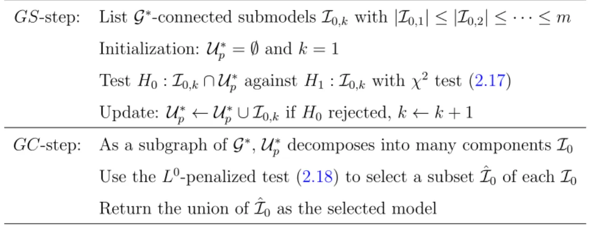
GS-step: ListG∗-connected submodels I
0,k with |I0,1| ≤ |I0,2| ≤ · · · ≤m Initialization: U∗
p =∅ and k = 1
TestH0 :I0,k∩ Up∗ against H1 :I0,k with χ2 test (2.17) Update: U∗
p ← Up∗∪ I0,k if H0 rejected,k ←k+ 1 GC-step: As a subgraph ofG∗, U∗
p decomposes into many componentsI0 Use the L0-penalized test (2.18) to select a subset ˆI0 of eachI0 Return the union of ˆI0 as the selected model
Table 2.1: Graphet Screening Algorithm
2.3 A BLOCKWISE EXAMPLE: NON-OPTIMAILITY OF SUBSET
SELECTION AND THE LASSO AND THE OPTIMALITY OF GRAPHLET SCREENING
Subset selection (also called theL0-penalization method) is a well-known method for variable selection, which selects variables by minimizing the following functional:
1 2kY −Xβk 2+1 2(λss) 2kβk 0, (2.20)
where kβkq denotes the Lq-norm, q ≥ 0, and λss > 0 is a tuning parameter. The AIC, BIC, and RIC are methods of this type [1,42, 19]. Subset selection is believed to have good “theoretic property”, but the main drawback of this method is that it is computationally NP hard. To overcome the computational challenge, manyrelaxationmethods are proposed, including but are not limited to the lasso [9,43], SCAD [17], MC+ [50], and Dantzig selector [8]. Take the lasso for example. The method selects variables by minimizing the following functional:
1
2kY −Xβk 2+λ
where theL0-penalization is replaced by theL1-penalization, so the functional is convex and the optimization problem is solvable in polynomial time under proper conditions.
Somewhat surprisingly, subset selection is generallyrate non-optimalin terms of selection errors. This sub-optimality of subset selection is due to its lack of flexibility in adapting to the “local” graphic structure of the design variables. Similarly, other global relaxation methods are sub-optimal as well, as the subset selection is the “idol” these methods try to mimic. To save space, we only discuss subset selection and the lasso, but a similar conclusion can be drawn for SCAD, MC+, and Dantzig selector.
For mathematical simplicity, we illustrate the point with an idealized regression model where the Gram matrix G=X0X is diagonal block-wise and has the following form
G(i, j) = 1{i=j}+h0·1{|j−i|= 1, max(i, j) is even}, |h0|<1, 1≤i, j ≤p. (2.22) Using an idealized model is mostly for technical convenience, but the non-optimality of subset selection or the lasso holds much more broadly than what is considered here. Since our goal is to show such methods are non-optimal, using a simple model is sufficient: if a procedure is non-optimal in an idealized case, we can not expect it to be optimal in a more general context.
At the same time, we continue to model β with the Asymptotic Rare and Weak model ARW(ϑ, r, a, µ), but where we relax the assumption ofµ∈Θ∗p(τp, a) to that ofµ∈Θp(τp) so that the strength of each signal≥τp(but there is no upper bound on the strength). Consider a variable selection procedure ˆβ?, where ? =gs, ss, lasso, representing Graphlet Screening, subset selection, and the lasso (where the tuning parameters for each method are ideally set; for the worst-case risk considered below, the ideal tuning parameters depend on (ϑ, r, p, h0) but do not depend on µ). For some exponents ρ? =ρ?(ϑ, r, h0) that does not depend on p, it is seen that for large p, the worst-case Hamming selection error of ˆβ? has the form of
sup
{µ∈Θp(τp)}
Hp( ˆβ?;p, µ, G) = Lpp1−ρ?(ϑ,r,h0).
Here,Hpis slightly different from that in Section2.1.4since the settings are slightly different. We now study ρ?(ϑ, r, h0). Towards this end, we first introduce
ρ(3)lasso(ϑ, r, h0) = (2|h0|)−1[(1−h20) √ r− q (1−h2 0)(1− |h0|)2r−4|h0|(1− |h0|)ϑ] 2 ,
and ρ(4)lasso(ϑ, r, h0) =ϑ+ (1− |h0|)3(1 +|h0|) 16h2 0 (1 +|h0|) √ r− q (1− |h0|)2r−4|h0|ϑ/(1−h20) 2 . We then let ρ(1)ss(ϑ, r, h0) = 2ϑ, r/ϑ≤2/(1−h20) [2ϑ+ (1−h2 0)r]2/[4(1−h20)r], r/ϑ >2/(1−h20) , ρ(2)ss(ϑ, r, h0) = 2ϑ, r/ϑ≤2/(1− |h0|) 2[p2(1− |h0|)r− p (1− |h0|)r−ϑ]2, r/ϑ >2/(1− |h0|) , ρ(1)lasso(ϑ, r, h0) = 2ϑ, r/ϑ≤2/(1− |h0|)2 ρ(3)lasso(ϑ, r, h0), r/ϑ >2/(1− |h0|)2 , and ρ(2)lasso(ϑ, r, h0) = 2ϑ, r/ϑ≤(1 +|h0|)/(1− |h0|)3 ρ(4)lasso(ϑ, r, h0), r/ϑ >(1 +|h0|)/(1− |h0|)3 . The following theorem is proved in Section A.1.2.
Theorem 2.3.1. Fix ϑ ∈(0,1) and r >0 such that r > ϑ. If G satisfies (2.22), then
ρgs(ϑ, r, h0) = min (ϑ+r) 2 4r , ϑ+ (1− |h0|) 2 r, 2ϑ+ {[(1−h20)r−ϑ]+}2 4(1−h2 0)r , (2.23) ρss(ϑ, r, h0) = min (ϑ+r) 2 4r , ϑ+ (1− |h0|) 2 r, ρ (1) ss(ϑ, r, h0), ρ(2)ss(ϑ, r, h0) , (2.24) and ρlasso(ϑ, r, h0) = min{ (ϑ+r)2 4r , ϑ+ (1− |h0|)r 2(1 +p1−h2 0) , ρ(1)lasso(ϑ, r, h0), ρ (2) lasso(ϑ, r, h0) . (2.25)
ϑ/r/h0 .1/11/.8 .3/9/.8 .5/4/.8 .1/4/.4 .3/4/.4 .5/4/.4 .1/3/.2 .3/3/.2 ?=gs 1.1406 1.2000 0.9000 0.9907 1.1556 1.2656 0.8008 0.9075 ?=ss 0.8409 0.9047 0.9000 0.9093 1.1003 1.2655 0.8007 0.9075 ?=lasso 0.2000 0.6000 0.7500 0.4342 0.7121 1.0218 0.6021 0.8919
Table 2.2: The exponents ρ?(ϑ, r, h0) in Theorem 2.3.1, where ?=gs, ss, lasso.
It can be shown that ρgs(ϑ, r, h0) ≥ ρss(ϑ, r, h0) ≥ ρlasso(ϑ, r, h0), where depending on the choices of (ϑ, r, h0), we may have equality or strict inequality (note that a larger expo-nent means a better error rate). This fits well with our expectation, where as far as the convergence rate is concerned, Graphlet Screening is optimal for all (ϑ, r, h0), so it beats the subset selection, which in turn beats the lasso. Table 2.2 summarizes the exponents for some representative (ϑ, r, h0). It is seen that differences between these exponents become increasingly prominent whenh0 increase and ϑ decrease.
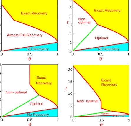
Similar to that in Section 2.1.5, each of these methods has a phase diagram, where the phase space partitions into three regions: Region of Exact Recovery, Region of Almost Full Recovery, and Region of No Recovery. Interestingly, the separating boundary for the last two regions are the same for three methods, which is the line r = ϑ. The boundary that separates the first two regions, however, vary significantly for different methods. For any h0 ∈(−1,1) and?=gs, ss, lasso, the equation for this boundary can be obtained by setting ρ?(ϑ, r, h0) = 1 (the calculations are elementary so we omit them). Note that the lower the boundary is, the better the method is, and that the boundary corresponding to the lasso is discontinuous at ϑ= 1/2. Compare the phase diagrams in Figure 2.1.
Subset selection and the lasso are rate non-optimal for they are so-called one-step or
non-adaptive methods [31], which use only one tuning parameter, and which do not adapt to the local graphic structure. The non-optimality can be best illustrated with the diagonal block-wise model presented here, where each block is a 2×2 matrix. Correspondingly, we can partition the vector β into many size 2 blocks, each of which is of the following three
types (i) those have no signal, (ii) those have exactly one signal, and (iii) those have two signals. Take the subset selection for example. To best separate (i) from (ii), we need to set the tuning parameter ideally. But such a tuning parameter may not be the “best” for separating (i) from (iii). This explains the non-optimality of subset selection.
Seemingly, more complicated penalization methods that use multiple tuning parameters may have better performance than the subset selection and the lasso. However, it remains open how to design such extensions to achieve the optimal rate for general cases. To save space, we leave the study along this line to the future.
0 0.5 1 0 1 2 3 4 5 6 ϑ r Exact Recovery
Almost Full Recovery
No Recovery 0 0.5 1 0 1 2 3 4 5 6 ϑ r Exact Recovery Optimal Non− optimal No Recovery 0 0.5 1 0 1 2 3 4 5 6 ϑ r Exact Recovery Optimal Non−optimal No Recovery 0 0.5 1 0 5 10 15 20 ϑ r Exact Recovery Optimal Non−optimal No Recovery
Figure 2.1: Phase diagrams for Graphlet Screening (top left), subset selection (top right), and the lasso (bottom; zoom-in on the left and zoom-out on the right), where h0 = 0.5.
2.4 SIMULATIONS
We conducted a small-scale simulation study to investigate the numerical performance of Graphlet Screening and compare it with the lasso. The subset selection is not included for comparison since it is computationally NP hard. We consider experiments for both random design and fixed design, where as before, the parameters (p, τp) are tied to (ϑ, r) byp =p−ϑ and τp =
p
2rlog(p) (we assume σ= 1 for simplicity in this section). The experiments with random design contain the following steps.
1. Fix (p, ϑ, r, µ,Ω) such that µ ∈Θp(τp). Generate a vector b = (b1, b2, . . . , bp)0 such that bi
iid
∼Bernoulli(p), and set β =b◦µ.
2. Fix κ and letn =np =pκ. Generate an n×p matrix with iid rows from N(0,(1/n)Ω). 3. Generate Y ∼N(Xβ, Ip), and apply Graphlet Screening and the lasso.
4. Repeat 1-3 independently, and record the average Hamming distances.
The steps for fixed design experiments are similar, except for that np =p and X = Ω1/2. Graphlet Screening uses tuning parameters (m,Q, ugs, vgs). We setm = 3 for our exper-iments, which is usually large enough due to signal sparsity. The choice ofQ is not critical, as long as the corresponding parameterq satisfies (1.26 [32]). Numerical studies below (e.g. Experiment 4a) support this point. In principle, the optimal choices of (Q, ugs, vgs) depend on the unknown parameters (p, τp), and how to estimate them in general settings is a lasting open problem (even for linear models with orthogonal designs). Fortunately, our studies (e.g. Experiment 4b-4d) show that mis-specifying parameters (p, τp) by a reasonable amount does not significantly affect the performance of the procedure. For this reason, in most experi-ments below, we set the tuning parameters in a way by assuming (p, τp) as known. To be fair in comparison, we also set the tuning parameters of the lasso ideally assuming (p, τp) as known. We use glmnetpackage [22] to perform lasso.
The simulations contain 4 different experiments which we now describe separately.
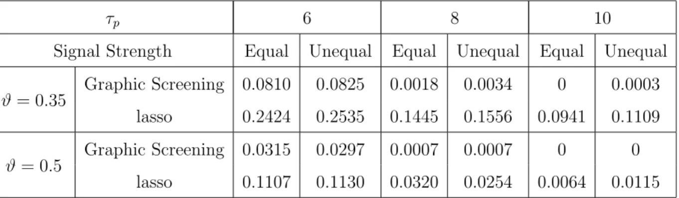
Experiment 1. In this experiment, we investigate how different choices of signal vector β affect the comparisons of two methods. We use a random design model, and Ω is a symmetric tri-diagonal correlation matrix where the vector on each sub-diagonal consists of blocks of
(.4, .4,−.4)0. Fix (p, κ) = (0.5×104,0.975) (note n = pκ ≈ 4,000). We let
p = p−ϑ with ϑ ∈ {0.35,0.5} and let τp ∈ {6,8,10}. For each combination of (p, τp), we consider two choices of µ. For the first choice, we let µ be the vector where all coordinates equal to τp (note β is still sparse). For the second one, we let µ be the vector where the signs of µi = ±1 with equal probabilities, and |µi|
iid
∼ 0.8ντp + 0.2h, where ντp is the point mass at τp and h(x) is the density of τp(1 +V /6) with V ∼χ21. For Graphlet Screening, the tuning parameters (m, ugs, vgs) are set as (3,p2 log(1/p), τp), and the tuning parameter q in Q
are set as maximal possible value satisfying the optimality conditions of GS. The average Hamming errors for both procedures across 40 repetitions are tabulated in Table 2.3.
τp 6 8 10
Signal Strength Equal Unequal Equal Unequal Equal Unequal ϑ= 0.35
Graphic Screening 0.0810 0.0825 0.0018 0.0034 0 0.0003 lasso 0.2424 0.2535 0.1445 0.1556 0.0941 0.1109 ϑ = 0.5 Graphic Screening 0.0315 0.0297 0.0007 0.0007 0 0
lasso 0.1107 0.1130 0.0320 0.0254 0.0064 0.0115
Table 2.3: Ratios between the average Hamming errors and pp (Experiment 1), where “Equal” and “Unequal” stand for the first and the second choices of µ, respectively.
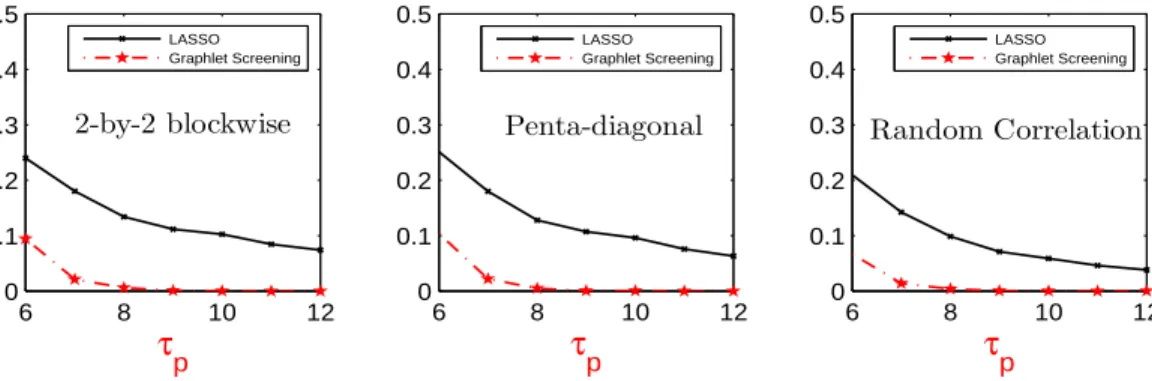
Experiment 2. In this experiment, we generateβ the same way as in the second choice of Experiment 1, and investigate how different choices of design matrices affect the performance of the two methods. Setting (p, ϑ, κ) = (0.5×104,0.35,0.975) and τ
p ∈ {6,7,8,9,10,11,12}, we use Gaussian random design model for the study. For each method, the tuning parameters are set in the same way as in Experiment 1. The experiment contains 3 sub-experiments 2a-2c. For each sub-experiment, the average Hamming errors of 40 repetitions are reported in Figure 2.2.
In Experiment 2a, we set Ω as the symmetric diagonal block-wise matrix, where each block is a 2×2 matrix, with 1 on the diagonals, and ±0.5 on the off-diagonals (the signs alternate across different blocks).
In Experiment 2b, we set Ω as a symmetric penta-diagonal correlation matrix, where the main diagonal are ones, the first sub-diagonal consists of blocks of (.4, .4,−.4)0, and the second sub-diagonal consists of blocks of (.05,−.05)0.
In Experiment 2c, we generate Ω as follows. First, we generate Ω using the function
sprandsym(p,K/p) in matlab. We then set the diagonals of Ω to be zero, and remove some of entries so that Ω is K-sparse for a pre-specified K. We then normalize each non-zero entry by the sum of the absolute values in that row or that column, whichever is larger, and multiply each entry by a pre-specified positive constant A. Last, we set the diagonal elements to be 1. We choose K = 3 and A= 0.7, draw 5 different Ω with this method, and for each of them we repeat the simulation 10 times independently.
The results suggest that Graphlet Screening is consistently better than the lasso.
6 8 10 12 0 0.1 0.2 0.3 0.4 0.5 τp 2-by-2 blockwise LASSO Graphlet Screening 6 8 10 12 0 0.1 0.2 0.3 0.4 0.5 τp Penta-diagonal LASSO Graphlet Screening 6 8 10 12 0 0.1 0.2 0.3 0.4 0.5 τp Random Correlation LASSO Graphlet Screening
Figure 2.2: x-axis: τp. y-axis: ratios between the average Hamming errors andpp (from left to right: Experiment 2a, 2b, and 2c).
Experiment 3. In this experiment, we investigate what are the minimum signal strength levels τp required by Graphlet Screening and the lasso to yield exact recovery, respectively. Fixing p= 104, we let p = p−ϑ for ϑ= 0.25,0.45,0.65, and let τp ∈ {5,6,7,8,9,10,11,12}. We use a fixed design model where Ω is the block-wise matrix as in Experiment 2a. For each pair of (p, τp), we generate β as in the second choice of Experiment 1. The tuning parameters for Graphlet Screening and the lasso are set in the same way as in Experiment 1. The average Hamming errors across 20 repetitions are tabulated in Table.2.4.
Suppose we say a method yields ‘exact recovery’ if the average Hamming error ≤ 3. Then the minimum τp for Graphlet Screening to yield exact recovery is τp ≈9, but that for the lasso is much larger (≥ 12). For larger ϑ, the differences are less prominent, but the minimumτp for Graphlet Screening to yield exact recovery is consistently smaller than that of the lasso. τp 5 6 7 8 9 10 11 12 ϑ = 0.25 Graphic Screening 58 21.4 9.2 3.5 3 1.8 1.0 0.6 lasso 75.2 34.4 21.6 15 14.3 12.6 10.1 8.9 ϑ = 0.45 Graphic Screening 11 3.7 0.7 0.2 0.1 0 0 0 lasso 13.9 5.2 1.3 0.6 0.1 0.4 0.2 0.2 ϑ = 0.65 Graphic Screening 3.4 0.8 0.1 0.1 0 0 0 0 lasso 3.7 1 0.3 0.1 0 0 0 0
Table 2.4: Comparison of average Hamming errors (Experiment 3).
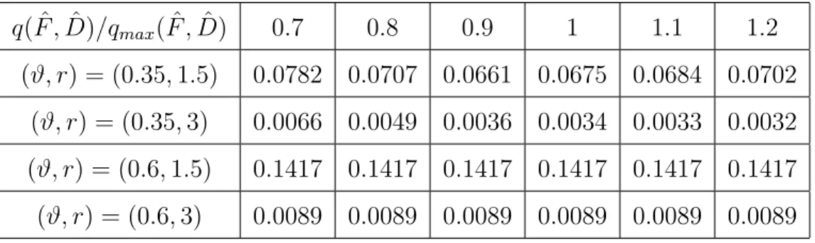
Experiment 4. In this experiment, we investigate how sensitive Graphlet Screening is with respect to the tuning parameters. The experiment contains 4 sub-experiments, 4a-4d. In Experiment 4a, we investigate how sensitive the procedure is with respect to the tuning parameter q in Q (recall that the main results hold as long as q fall into the range given in (1.26 [32]), where we assume (p, τp) are known. In Experiment 4b-4d, we mis-specify (p, τp) by a reasonably small amount, and investigate how the mis-specification affect the performance of the procedure. For the whole experiment, we choose β the same as in the second choice of Experiment 1, and Ω the same as in Experiment 2b. We use a fixed design model in Experiment 4a-4c, and a random design model in Experiment 4d. For each sub-experiment, the results are based on 40 independent repetitions. We now describe the sub-experiments with details.
In Experiment 4a, we chooseϑ ∈ {0.35,0.6}and r∈ {1.5,3}. In Graphlet Screening, let qmax =qmax( ˆD,Fˆ) be the maximum value of q satisfying (1.26 [32]). For each combination of (ϑ, r) and ( ˆD,Fˆ), we choose q( ˆD,Fˆ) = qmax( ˆD,Fˆ) × {0.7,0.8,0.9,1,1.1,1.2} for our
experiment. The results are tabulated in Table 2.5, which suggest that different choices of q have little influence over the variable selection errors. We must note that the larger we set q( ˆD,Fˆ), the faster the algorithm.
q( ˆF ,D)/qmax( ˆˆ F ,D)ˆ 0.7 0.8 0.9 1 1.1 1.2 (ϑ, r) = (0.35,1.5) 0.0782 0.0707 0.0661 0.0675 0.0684 0.0702
(ϑ, r) = (0.35,3) 0.0066 0.0049 0.0036 0.0034 0.0033 0.0032 (ϑ, r) = (0.6,1.5) 0.1417 0.1417 0.1417 0.1417 0.1417 0.1417 (ϑ, r) = (0.6,3) 0.0089 0.0089 0.0089 0.0089 0.0089 0.0089
Table 2.5: Ratios between the average Hamming errors of Graphlet Screening and pp (Ex-periment 4a).
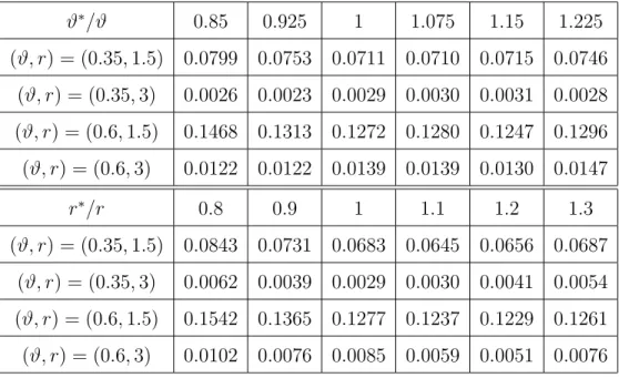
In Experiment 4b, we use the same settings as in Experiment 4a, but we assumeϑ(and so p) is unknown (the parameterris assumed as known, however), and letϑ∗ is the misspecified value ofϑ. We take ϑ∗ ∈ϑ× {0.85,0.925,1,1.075,1.15,1.225} for the experiment.
In Experiment 4c, we use the same settings as in Experiment 4a, but we assumer(and so τp) is unknown (the parameterϑis assumed as known, however), and letr∗ is the misspecified value ofr. We take r∗ =r× {0.8,0.9,1,1.1,1.2,1.3} for the experiment.
In Experiment 4b-4c, we run Graphlet Screening with tuning parameters set as in Exper-iment 1, exceptϑ or r are replaced by the misspecified counterpartsϑ∗ and r∗, respectively. The results are reported in Table 2.6, which suggest that the misspecifications have little effect as long asr∗/r and ϑ∗/ϑ are reasonably close to 1.
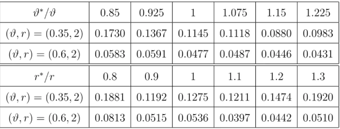
In Experiment 4d, we re-examine the misspecification issue with a random design. We use the same settings as in Experiment 4b and Experiment 4c, except for (a) while we use the same Ω as in Experiment 4b, the design matrixX are generated according to the random design model as in Experiment 2b, and (b) we only investigate for the case of r = 2 and ϑ∈ {0.35,0.6}. The results are summarized in Table2.7, which is consistent with the results in 4b-4c.
ϑ∗/ϑ 0.85 0.925 1 1.075 1.15 1.225 (ϑ, r) = (0.35,1.5) 0.0799 0.0753 0.0711 0.0710 0.0715 0.0746 (ϑ, r) = (0.35,3) 0.0026 0.0023 0.0029 0.0030 0.0031 0.0028 (ϑ, r) = (0.6,1.5) 0.1468 0.1313 0.1272 0.1280 0.1247 0.1296 (ϑ, r) = (0.6,3) 0.0122 0.0122 0.0139 0.0139 0.0130 0.0147 r∗/r 0.8 0.9 1 1.1 1.2 1.3 (ϑ, r) = (0.35,1.5) 0.0843 0.0731 0.0683 0.0645 0.0656 0.0687 (ϑ, r) = (0.35,3) 0.0062 0.0039 0.0029 0.0030 0.0041 0.0054 (ϑ, r) = (0.6,1.5) 0.1542 0.1365 0.1277 0.1237 0.1229 0.1261 (ϑ, r) = (0.6,3) 0.0102 0.0076 0.0085 0.0059 0.0051 0.0076
Table 2.6: Ratios between of the average Hamming error of the Graphlet Screening and pp (Experiment 4b (top) and Experiment 4c (bottom)).
2.5 DISCUSSION AND FUTURE WORK
In this chapter, we focus on the regime where the Gram matrix is sparse. A further exten-sion of the GS methodology would be the cases where the Gram matrix is not sparse, but sparsifiable. One such case is when there are a few hot hubs in GOSD. Once we find these hubs, the conditional covariance structure of the other variables may be sparse or blockwise. Another interesting direction of future research is the extension of the GS methodology to more general models such as logistic regression.
ϑ∗/ϑ 0.85 0.925 1 1.075 1.15 1.225 (ϑ, r) = (0.35,2) 0.1730 0.1367 0.1145 0.1118 0.0880 0.0983 (ϑ, r) = (0.6,2) 0.0583 0.0591 0.0477 0.0487 0.0446 0.0431 r∗/r 0.8 0.9 1 1.1 1.2 1.3 (ϑ, r) = (0.35,2) 0.1881 0.1192 0.1275 0.1211 0.1474 0.1920 (ϑ, r) = (0.6,2) 0.0813 0.0515 0.0536 0.0397 0.0442 0.0510
Table 2.7: Ratios between the average Hamming errors of Graphlet Screening and pp (Ex-periment 4d).
3.0 EXPLOIT THE DEPENDENCY AMONG THE SIGNALS
3.1 INTRODUCTION
Consider a Stein’s normal means model
Y =β+z, (3.1)
whereY, β and z are p×1 vectors, z ∼N(0, Ip). Hereβ = (β1, β2, ..., βp)0, ifβi 6= 0, we call it a signal, otherwise, a noise. The mean vectorβ is unknown, but presumably sparse, which means most of the coordinates of β are zeroes. We define a length pvector b = (b1, . . . , bp)0 as bi = 1{βi 6= 0} for i= 1, . . . , p. Then b is the indicator of the signals. The main goal of this paper is to estimate b, or equivalently, to find all the non-zero coordinates of β.
Though (3.1) is very simple, it has profound implications in many statistical problems.
• Linear regression. Consider Y = Xβ +z, where z ∼ N(0, In), X is the n×p design matrix, and the Gram matrix X0X ≈ Ip. Let ˜Y = X0Y, then approximately we have
˜
Y =β+ ˜z, where ˜z ∼N(0, Ip).
• Classification. Consider a two class classification problem where the training set has n subjects and p variables and X = [X1, . . . , Xp] is the n ×p feature matrix. We are interested in building an effective classifier with a small portion of the variables. We can define an length p vector Y where for i = 1, . . . , p, Yi is the standardized difference of the sample means of Xi between the two classes. When bothp andn are large (possibly pn), approximatelyY satisfies (3.1). Intuitively, ifβi 6= 0, thenXishould be included to the classifier. If βi = 0, Xi may not be necessary for classification.
3.1.1 Structured sparsity in the paradigm of rare and weak signals
We focus on the regime where the signals are both rare and weak. The rarity (or sparsity) is a well-accepted concept. But signal weakness is a much neglected notion until recently. Actually, similar to the sparsity, signal weakness is also a natural phenomenon that usually arise from the issue of p n. Take the above high dimensional classification problem for example, when p n, some of the standardized two-sample means could be very noisy. In our model, signal weakness implies that the magnitudes of the non-zeros ofβare individually small or moderately large, and barely separable with the noise.
Most of the previous work on the rare and weak signals focus on the completely unstruc-tured case and do not take in interaction among the features into account. Recently, in the setting linear regression and classification, some works [21, 31, 32, 35] start to consider the correlation structure of the features. While these works are successful in their own regimes, what is still neglected is the dependency structure among the signals themselves. In this paper, we consider the variable selection problem when the signals depend on each other significantly.
3.1.2 Ising model: modeling the signal dependency
Let G be an undirected graph of dependency with p nodes, and each node is conditional independent to others given its neighbors. In our model (3.1), the signals depend on each other in a sense that if we know thatβi 6= 0, thenβj1, . . . , βni are more likely to be non-zeros, where {j1, . . . , jni} are the neighbors of node iin graph G. We also assume the dependency structure is sparse in a sense that the graph G is sparse or equivalently, for each node i, the size of its neighborhood ni is very small. In many application areas, the dependency among the sparse signals naturally exists, and the dependency structure is sparse and known, though the dependency strength may be unknown.
• Image analysis: In image analysis, it is of interest to recover the objects in a “dirty picture” [3]. Consider a toy example where there are only two colors, black and white. Assume that most area of the picture is white, then the signals (black pixels) are sparse. In this problem, if we know one pixel is black, the pixels near it are more likely to be
black. The simplest graphical presentation of the above observation would be a 2-d lattice, where the pixels are treated as nodes in the graph, and for each pixel, only the four pixels in its direct neighborhood are connected with it in the lattice graph. This graph is sparse.
• Network-based analysis in biology: In biology, genes and proteins interact in a compli-cated way. In the past two decades, various network databases have been built to model these interaction patterns, e.g genetic regulatory network, protein-protein interaction network and biological pathways. In most of the cases, each gene or protein only interact with a small portion of other genes or proteins, hence the network in biology is usual-ly sparse. In data anausual-lysis problems such as finding differentialusual-ly expressed genes(DE) between the tumor patients and the general population, it is believed that only a small portion of the human genes are DE, hence DE is sparse. In this problem, it is intuitive to believe that if we know one gene is related to cancer, then those genes that interact with it are more likely to be also related to cancer. Thus, the existing biological network information may be very useful in such problems, and can be integrated into the analysis as the known “data about data” [34, 48].
An immediate question would be how to incorporate such prior information on signal de-pendency into data analysis.
We tackle this problem from a generative model perspective. Recall thatbis the indicator of the locations of the signals, and as before, our primary goal is to estimate b. We model the dependency among the signals by modeling b as a sample from an Ising model. So that Y satisfies a hidden Ising model.
The Ising model is originally a mathematical model of ferromagnetism in statistical mechanics [29]. Nowadays, we use Ising model to denote a wide class of Binary Markov Random Field with a distribution
P(b =`) = 1 Zp(η,Ω) exp −η`0Ω` , (3.2)
where Ω is the weighted adjacency matrix of the encoded undirected graphG, and its diagonal elements are 10s. Zp(η,Ω) is the normalizing constant. We denote it as b ∼Ising(η,Ω). We
remark that when Ω =Ip,
bi iid
∼Bernoulli( 1
1 +eη); (3.3)
Hence the Ising model can be viewed as a multivariate bernoulli distribution that takes the pairwise interactions into account.
Roughly speaking, in (3.2), Ω controls the dependency strength among the signals and for given Ω, the parameter η controls the number of signals. In our setting, Ω is sparse and the locations of the non-zeros are known, but the values of the elements of Ω are unknown. The signals generated by an Ising model live in disjoint signal clusters which we will formally define In Section3.2.1. In Section 3.2.1, we show that under mild constraints, (3.2) is an appropriate generative model for the sparse signals with sparse dependency structure. It generates sparse signals living in short signal clusters in graph G that are isolated to each other, and the maximal cluster length has a constant upper bound except a negligible probability. We refer to such models as sparse Ising model.
3.1.3 Objective of the chapter
We are interested in the optimal variable selection for (3.1) where the signal is weak and b is an interdependent signal generated by a sparse Ising model. The objective of the paper is three-fold.
• To study the Ising model, and specify a class of sparse Ising model that appropriately models the sparse interdependent signals.
• To develop a variable selection procedure that is accurate and computationally affordable, and investigate its application in various statistical problems.
• To study the variable selection problem with interdependent signals and the rate of minimax Hamming distance, to characterize the difficulty level of the variable selection problem and the performance of the procedures by Hamming distance, and to show the optimality of the above procedure in the rate of convergence in Hamming distance and the phase diagram.
In the regime of the rare and weak signal, exact recovery of b is usually impossible. Instead of probability of exact support recovery or “oracle property”, Hamming distance is a
more appropriate measure for the performances of variable selection procedures. Hamming distance is the expected number of errors in estimating the support b. Two related notions are Hamming ratio and the phase diagram. The phase diagram is a graphical criterion for measuring the performance of variable selection procedures, which is appropriate in our rare and weak signal paradigm. Hamming ratio is the ratio of the Hamming distance and the expected number of signals, which we use as the measurement of the variable selection procedures in our numeric study.
3.1.4 Non-optimality of hard thresholding
When b is a sample from a bernoulli model, the signal is unstructured. In this case, as a corollary of the results in [31], the element-wise hard thresholding can separate the signal from the noise optimally in the Hamming distance, given that the uniform threshold is optimally set. The the optimal rate of the hard thresholding is the same as the rate of separating a signal singleton from pure noise. Thus, the success of hard thresholding in the unstructured case can be attributed to the fact that the signals are independent to each other. Generally speaking, hard thresholding could be optimal if most signals live as singletons.
When the signals are generated from a sparse Ising model, there are two different cases. In the first case, the signals are moderately sparse and the dependency strength is strong so that most signals live in short signal clusters with more than one nodes, e.g. pairs, triplets. Thus hard thresholding is not optimal since it ignores the dependency structure. In the second case, the signals are so sparse or the dependency strength is so weak such that most signals are still singletons. Thus hard thresholding may be still optimal in this case.
However, when the signal dependency is very weak, it may not be necessary to incorporate such information into analysis at all, no matter what signal model we intend to use. Only when the signal dependency is strong, a model for interdependent signals such as our sparse Ising model becomes important or even crucial in data analysis. Therefore, as long as the signal dependency is a major concern in data analysis, hard thresholding is not the optimal choice for variable selection.
3.1.5 Intractability and decomposability of the likelihood of the sparse Ising model
Viewing b as hidden states, maximizing the conditional probability P(b|Y) is the “funda-mentally correct” way to estimateb. However, even when the parameters of the Ising model are known, maximizing this probability may involve comparing all b ∈ {0,1}p, which is intractable in computation.
Though this problem is seemingly intractable, we can still maximize P(b|Y) approxi-mately. Recall that the sparse Ising model generates sparse signal living in short clusters that are isolated to each other. By the definition of the signals clusters, there is no other signal in the neighborhood of each cluster. Thus if we know the locations of these clusters, these clusters are independent to each other. Then the signal graph of the sparse Ising model is decomposable, and so is the likelihood of the sparse Ising model.
To see this, let Si, i= 1, . . . , M be a collection of the isolated connected subgraphs ofG that contains all the signal clusters, and for any subgraph B, letN(B) be the neighborhood of B in the graph G. There is no signal outside ∪M
i=1Si, and we have P(b|Y)∝P(bj = 0 for j /∈ ∪Mi=1Si|Y) M Y i=1 P(bSi|YSi, bj = 0 for j ∈N(Si)) (3.4) Then we can maximize P(b|Y) by maximizing P(bSi|YSi, bj = 0 for j ∈ N(Si)) separately for i= 1, . . . , M.
Example 1. We illustrate the decomposability with a toy example. In model (3.1)-(3.2), letp= 4, and Ω is a diagonal matrix whose non-zero off-diagonal elements are−1/2. Then,
P(b =`)∝exp " −η( 4 X i=1 `i− 3 X i=1 `i`i+1) # . If we know that b2 = 0, we have
P(b=`|b2 = 0)∝exp (−η`1)·exp [−η(`3+`4−`3`4)]. On the other hand, we know
P(b =`|Y)∝P(b=`) 4
Y
i=1