Bootstrap Tests in Bivariate VAR Process with Single Structural Change : Power versus Corrected Size and Empirical Illustration

(1)

GREQAM

Groupement de Recherche en Economie Quantitative d'Aix-Marseille - UMR-CNRS 6579 Ecole des Hautes Etudes en Sciences Sociales

Universités d'Aix-Marseille II et III

Document de Travail

n°2006-4

1 Bootstrap Tests in Bivariate VAR Process with

Single Structural Change: Power versus

Corrected Size and Empirical Illustration

Jamel JOUINI

September 2006

(2)

Bootstrap Tests in Bivariate VAR Process with Single Structural

Change: Power versus Corrected Size and Empirical Illustration

Jamel JOUINI

∗

GREQAM, Université de la Méditerranée, Marseille, France

F.S.E.G.N., E.S.S.A.I.T. and L.E.G.I.

Université 7 Novembre de Carthage, Tunisie

September 14, 2006

Abstract: This paper evaluates thefinite-sample performance of single structural change tests based on the asymptotic distribution and bootstrap procedures. In addition to the conventional case of stationary regressors, we consider nonstationary regressors and others characterized by the presence of a break in their structure. While our paper borrows the idea of assessing the performance of structural break tests from an other paper, ours is thefirst to examine and compare the power of such tests on the basis of corrected size by using graphical methods. We endeavour to see whether some conclusions, obtained for some tests, remain again valid for others based on an other type of processes. Some bootstrap procedures quasi-perfectly correct the size distortions of their asymptotic counterparts and have the same power performance as them on the corrected size basis; property often diﬃcult to obtain. We

finally propose a modelling strategy to study the relationship between U.S. interest rates. The results show that such relationship has been altered by a regime-shift located at the beginning of the 1980s.

Key-words: Break date, Bootstrap techniques, Graphical methods, Selection procedures. JEL Classification: C20.

1. Introduction

In diversefields of application, many time series might exhibit the phenomenon of structural change which is of capital importance in economics and econometrics. The problem consists in testing the null hypothesis of structural stability against the alternative of instability. Under the alternative hypothesis, we can have one break or more. The literature addressing thefirst issue is huge. Indeed, Chow (1960) was the first who considered a classic F test allowing to test for single structural

∗_{Jamel JOUINI, Faculté des Sciences Economiques et de Gestion, Campus Universiatire Mrezgua, 8000 Nabeul,}

Tunisie. Tel.: +216 72 232 205; fax: +216 72 232 318; E-mail: [email protected].

(3)

change when the break point is known a priori. Quandt (1960) extends the analysis of Chow

(1960) to the case of unknown break date. Indeed, he computes a sequence of Chow statistics for all possible break dates contained in a restricted interval since we cannot consider break dates too close to the boundaries of the sample, as there aren’t enough observations to identify all the subsample parameters. The estimated break point is the one that maximizes the Chow test. In the same context, some important tests are the "supremum" tests of Andrews(1993), and the related "exponential" and "average" tests of Andrews and Ploberger (1994). They derive the asymptotic distributions which are useful to provide approximations to thefinite-sample distributions.1 These asymptotic distributions have been derived under the assumption of stationary regressors.2 This then precludes the presence of structural change in the marginal distribution of the regressors. In this context, Hansen (2000) remedies this deficiency and derives the asymptotic distributions of the test statistics. He finds that these distributions depend on structural change in the regressors. These asymptotic distributions may be an unreliable guide to finite-sample behavior and as a result the true levels of tests based on asymptotic critical values can be very diﬀerent from the nominal levels. An alternative approximation is the bootstrap distribution that gives evidence on the adequacy of tests and often provides a tractable way to reduce or eliminate finite-sample distortions of the sizes of statistical tests. In this context, Diebold and Chen (1996) consider a simulation study to obtain better size properties for the "supremum" tests of Andrews (1993) for single structural change using the nonparametric bootstrap procedure. Their study is a simple generalization of the study of Christiano (1992) who provides a bootstrap approximation to the distribution of the test statistic of Quandt (1960) to study the existence of structural change in the dynamics of U.S. aggregate output. In the same context and to obtain good size properties, Hansen (2000) introduces a fixed regressor bootstrap which leads to reasonable size properties in finite-samples. This bootstrap technique treats the regressors as if they are fixed (exogenous) even when they contain lagged dependent variables. It also allows for structural change in the regressors, including change in mean, change in trend function and change in exogenous stochastic trend function, and itfinally allows for heteroskedasticity in the errors.

In this paper, through Monte Carlo analysis, we examine and compare the size and power3 properties of a "supremum" test of Andrews (1993), and the related "exponential" and "average" tests of Andrews and Ploberger (1994) to see whether the bootstrap procedures reduce the error in rejection probability4 (size distortion) while conserving their power compared to that of their asymptotic counterparts. Since it can be diﬃcult to compare the power of alternative test statistics if they do not have the correct size, this comparative study is based on the graphical methods of

1

Note that Andrews et al. (1996) derive the finite-sample distribution for these tests, but the derivation only applies under a model withfixed regressors and normally distributed errors with known variance. In this paper, we explore thefinite-sample performance under much more general conditions.

2

Note that this cannot be a desirable hypothesis in practice.

3

The size of a test is the probability that it rejects the null hypothesis when it is true, while the power of a test is the probability that it rejects the null hypothesis when it is false.

4_{The error in rejection probability of a test is the di}_ﬀ_{erence between the actual and nominal probability of rejecting}

the null hypothesis when it is true.

(4)

Davidson and MacKinnon (1998) whose interest is the principle of size correction that allows to show the true power of tests instead of the nominal power, and hence to examine accurately the properties of the tests. We consider, in addition to the conventional case of stationary regressors, nonstationary regressors and others characterized by the presence of regime-shift in their structure. While some single structural change tests enjoy certain optimality properties in many cases, little is known about their comparative power properties under other conditions. In this paper, we attempt to study this point based on a bivariate VAR(2)process. To illustrate empirically the usefulness of all the procedures, we propose a modelling strategy to study the relationship between U.S. interest rates, and to detect an eventual break date in this relationship.5

The remainder of the paper is organized as follows. Section 2 presents the basic model and the estimation method allowing to estimate the regression coeﬃcients and the break date. Section

3 defines the "supremum" test of Andrews (1993), and the related "exponential" and "average" tests of Andrews and Ploberger (1994). In section 4, we introduce the bootstrap technique and the relating basic concepts being useful to carry out the simulation experiments. Section5defines the graphical methods of Davidson and MacKinnon (1998), namely the P value Plots, P value Discrepancy Plots and Size-Power Curves. Monte Carlo evidence on the size and power performance of both asymptotic and bootstrap approximations is given in section 6. The results indicate that the parametric and nonparametric bootstrap techniques outperform the asymptotic approximation since the bootstrap tests show more accurate size and the same power properties on the corrected size basis as their asymptotic counterparts. Thus, getting the size right and achieving high power are possible tasks. Note that this property is often diﬃcult to obtain when evaluating the performance of tests in terms of size and power. Another feature of substantial importance is that the Hansen’s

(2000) bootstrap procedures are sometimes inadequate. This then calls these procedures into question. We also study the eﬀect of change of the error distribution on the performance of the testing procedures. Section7reports an empirical application using U.S. interest rates to illustrate the usefulness of all the procedures in terms of selection of a break date in the data. The results show that the relationship between the interest rates has been altered by a break located in1981:5. Some economic explanations are provided to highlight the underlying factors that fostered the change and altered the relationship between the considered series. Section8 concludes the paper. The diﬀerent graphs of the simulation study are reported in Appendices A and B, and the graphics of the interest rates are presented in Appendix C.

2. The model and estimation method

Let us consider the following linear regression model:

yt=      x0_tδ+ut, x0_t(δ+θ) +ut, if 1_≤t_≤k0, if k0 < t≤T, (2.1) 5

It is well known that a proper treatment of parameter changes can be useful in uncovering the underlying factors that fostered the changes and altered a relationship between economic variables.

(5)

where yt is the dependent variable, xt is a m-vector of regressors, δ is the vector of regression coeﬃcients, θ represents the magnitude of change,k0 is the break date, and ut is the disturbance that has a distributionD¡0, σ2¢_{, with}_σ2_<_∞_{. The break point}_k

0is explicitly treated as unknown

and is contained in the interval [k1, k2] which is defined to restrict the break date to be bounded

from the boundaries of the sample, as there are not enough observations to identify the parameters of the two subsamples. When testing for single structural change, we are not concerned with the distribution of xt. Thus, the problem of structural change in the model (2.1) does not take into account the nature of the regressors; stationary or nonstationary. We are then interested in testing H0 :θ = 0versus H1 :θ 6= 0. In other words, we test the null hypothesis of stability against the

alternative hypothesis of a single structural change. Under the null hypothesis, the model(2.1)becomes

yt=x0tδ+ut, t= 1, . . . , T, (2.2) which does not depend on the break date k0. The estimation method considered is that based on

the least-squares principle (Bai,1997). Indeed, under the null hypothesis the ordinary least-squares (OLS) estimates areˆδ, the residualsuˆt, and the estimator of the varianceσˆ2 = (T−m)−1PTt=1uˆ2t. Under the alternative hypothesis, the model can be written as

yt=x0tδ+xt0θI(t > k0) +ut, (2.3) where I(_·) is an indicator function that takes the value 1 if its argument is true and 0 otherwise. For a givenk, the model(2.3)can be estimated by OLS to get the estimates³ˆδk,ˆθk

´

, the residuals

ˆ

utk, and the estimator of the variance σˆ2_k = (T₋2m)−1PT_t₌₁uˆ2_tk. The break date estimator kˆ is such that ˆ k= arg min k σˆ 2 k. (2.4)

Finally, the OLS estimates of the regression coeﬃcients and the residuals are respectively ˜δ = ˆδ_kˆ,

˜

θ= ˆθˆ_k, andut˜ = ˆu_tˆ_k.

3. The structural change tests

Chow (1960) was the first who considered a classic F test allowing to test for single structural change when the break date is known a priori. He uses the following Wald statistic:

Fk=

(T₋m) ˆσ2₋(T ₋2m) ˆσ2_k

ˆ

σ2_k . (3.1)

This test statistic is equivalent to the likelihood ratio statistic when the errorsutarei.i.d. N¡0, σ2¢. In this paper, we are interested in testing the null hypothesis of stability when the true break date k0 is unknown a priori.

(6)

Quandt(1960)extends the analysis of Chow(1960) and proposes a likelihood ratio test equiv-alent to

SupFT = sup

k∈[k1,k2]

Fk. (3.2)

Note that the break date corresponding to the maximal value of the sequence of the statisticsFkfor all the possible break dates contained in the interval[k1, k2] constitutes an estimator of the break

point.6 The asymptotic distribution of the test statisticSupFT has been derived in Andrews(1993)

for stationary regressors. Hansen (2000) derives the asymptotic distribution of the test statistic SupFT when the marginal distribution of the regressors is aﬀected by a structural change. Hefinds the same distribution as Andrews(1993), but it depends on

λ∗ =π∗₂(1₋π∗₁)/[π∗₁(1₋π∗₂)], (3.3) rather than

λ=π2(1−π1)/[π1(1−π2)], (3.4)

as found by Andrews(1993). Note that π∗

1=υ(π1),π2∗ =υ(π2), and υ is a function such that

υ(r) = [r+ω(r₋_κ)I(r_≥_κ)]/[1 +ω(1₋_κ)], (3.5) where ω is the magnitude of change in the regressors, _κ = [ T] is the corresponding break date, and π1 and π2 are such thatπ1 =k1/T and π2 =k2/T. Note thatλ∗ is a function only of π∗1 and

π∗₂, the relative information cumulated in the regressors at the timesπ1 and π2. From Table 1 of

Andrews(1993), the asymptotic critical values forSupFT are increasing inλ. Thus, ifλ∗ > λ, then the statisticSupFT has high tendency to reject the null hypothesis if Andrews’ critical values are used. On the other hand, if λ∗ < λ, then this statistic tends to reject too infrequently, reducing power.7 In our simulation experiments presented in section 6 (π1 = 0.15, π2 = 0.85, ω = 3 and

= 0.5), λ∗ = 49.61 > λ= 32.11 and thus the statistic SupFT using the Andrews’ critical values has severe size distortions as shown by the P value plots in Figure8.

Andrews and Ploberger (1994) suggest two related tests, namely the "exponential" and "aver-age" tests ExpFT = ln Z k exp (Fk/2)dw(k), (3.6) AveFT = Z k Fkdw(k), (3.7)

wherew is a measure putting weight 1/(k2−k1) on each integer kin the interval [k1, k2].

6_{This estimator is the same as that obtained by minimizing the sum of squared residuals.} 7

Hansen(2000) plotsλ∗ as a function of κ for four positive values ofω,π1 = 0.15and π2 = 0.85. For each ω,

λ∗_{is maximized at} ₌_π

1 and minimized at =π2. Asωincreases,λ∗can become arbitrarily large. The sampling

implications is that theSupFT statistic can have arbitrarily large size distortion.

(7)

The asymptotic distributions of all the above-mentioned test statistics are derived under the regressor stationarity hypothesis.8 Consequently, the nonstationarity and structural change in the marginal distribution of the regressors aﬀect the asymptotic distributions of these statistics, and then the critical values tabulated based on these distributions are not valid. This then justifies the recourse to the bootstrap as an approximation method of the distributions in such cases.

In this paper, we are interested in comparing the size and power of the asymptotic and boot-strapping versions of theSupFT,ExpFT andAveFT tests. For the power, the attention is particu-larly paid to the location of the break and distance of the alternative from the null. Although, for example, theExpFT and AveFT tests enjoy certain optimality properties in large samples, little is known about their comparative power properties under other conditions.

4. Bootstrap tests

Since the asymptotic tests may, in finite-samples, be biased in the sense that they have empir-ical sizes that diﬀer from their nominal ones, an alternative approach is necessary. One such distribution-free method is the bootstrap method, introduced by Efron (1979). The bootstrap is based on the idea that the sample is a good representation of the underlying population distribu-tion. As a result, the population distribution can be approximated by drawing samples repeatedly (so-called, resamples) from the original sample.9 _{It is well known that the bootstrap procedure can} successfully approximate the finite-sample distribution especially when the statistic is asymptoti-cally pivotal (Horowitz,1997; and Hall,1992).

A main feature of bootstrap tests is that, under certain conditions, their actual sizes will converge to the true ones faster than asymptotic tests and at times converge considerably faster. This paper proposes the following procedures for the structural change tests, to construct the bootstrapping distribution10 under the null hypothesis of stability.11

4.1. Standard procedures

The standard bootstrap procedure is as follows:

1. Compute the asymptotic test statistic in the usual way.

2. Estimate the model under the null hypothesis by the least-squares principle and construct the following bootstrap DGP:

8_{The work of Ploberger and Krämer} ₍₁₉₉₆₎ _{is a notable exception since the authors show that in the presence}

of general trends in the regressors, the asymptotic distribution of the CUSUM test is bounded by the asymptotic distribution in the case of stationary regressors.

9_{See Jeong and Maddala}₍₁₉₉₃₎_{or Horowitz}₍₁₉₉₄₎_{for a review of bootstrap methods in econometrics.}

1 0_{As we mentioned above the nonstationarity and structural change in the marginal distribution of the regressors}

aﬀect the asymptotic distributions of the test statistics in complicated ways. An alternative solution consists in using bootstrap methods to yield approximations to the distributions of the considered test statistics.

1 1_{The idea of constructing the bootstrap DGP under the null hypothesis is proposed by Beran}_{(1986), and Beran}

and Srivastava(1985).

(8)

y∗_t =x0_tˆδ+u∗_t, (4.1) whereˆδis the restricted parameter estimate. This DGP is just an element of the model(2.2)

using the parameters estimated under the null hypothesis.12 _{For the parametric bootstrap,} we have u∗_t _∼ Dˆ¡0,σˆ2¢ where σˆ2 = (T₋m)−1PT_t₌₁uˆ2_t. Note that without the normality assumption, it does not make sense to generate bootstrap errors from the normal distribution. Instead, we want to generate them nonparametrically by resampling with replacement from the residual vectoru˘=_{u˘t}Tt=1;

˘ ut= r T T₋m Ã ˆ ut− 1 T T X s=1 ˆ us ! . (4.2)

3. Based on these data, compute a bootstrap test statistic in exactly the same way as the real sample was used to compute the asymptotic statistic.

4.2. Hansen’s (2000) procedures

The standard bootstrap procedures need the joint modelling ofytand xtwhich require the correct specification of the marginal distribution (including any structural change). To ignore the marginal distribution of the regressors when generating bootstrap data, Hansen(2000)proposes two alterna-tive bootstrap procedures, called the homoskedastic bootstrap and the heteroskedastic bootstrap to yield approximations to the distributions of test statistics in the presence of nonstationarity and structural change in the regressors. These techniques treat the regressors xt as if they are fixed (exogenous) even when they contain lagged dependent variables, and allow for structural change in the regressors and heteroskedastic errors. The Hansen’s bootstrap techniques replicate the correct

first-order asymptotic distribution, but it is easy to see that in general the bootstrap does not (in any way) replicate the finite sample distribution of the data or the test statistics. The only ex-ception is when the regressorsxt are strictly exogenous and the errorsi.i.d. normal, in which case the homoskedastic bootstrap described below will yield exact inference.13 Consequently, caution should be applied when interpreting the bootstrap tests.

For the homoskedastic bootstrap, the data y∗ are generated by drawing observations from the N(0,1) distribution.14 To compute a realization of the bootstrap test statistic, we regress y∗ on xt to get ˆσ∗2, and we regress y∗ on xt and xtI(t > k) to get σˆ∗_k2. The heteroskedastic bootstrap consists in generating bootstrap datay∗ according toe∗_tu˜t, wheree∗t ∼i.i.d. N(0,1)andu˜tare the regression residuals defined in section 2. The bootstrap Wald statistic is then

1 2_{Note that all the parameter estimates are kept}_fi_{xed during the bootstrap replications, i.e. they are treated as}

the true population parameters.

1 3_{This is a well known property of bootstrap inference with an exactly pivotal statistic. For more details, see Hall}

(1994).

1 4_{It may be possible to use alternative distributions such as the empirical distribution function (EDF) of the}

residuals.

(9)

F_k∗ = (T−m) ˆσ

∗2

−(T₋2m) ˆσ∗_k2

ˆ

σ∗_k2 .

The method applies as well for the other tests. 4.3. Computation of bootstrap P value The bootstrap P value is computed as follows:

1. Draw B bootstrap samples from the above DGPs so as to obtain B bootstrap statistics. 2. The bootstrap P value, saypˆ∗, is then estimated by the proportion of bootstrap samples that

yield a statistic greater than the asymptotic statistic.15

We reject the null hypothesis if the bootstrap P value pˆ∗ is less thanα, the significance level of the test.

4.4. The bootstrap when the null hypothesis is false

We know that to obtain an exactfinite-sample distribution, it is preferred to construct the boot-strap DGP under the null hypothesis. When this hypothesis is false, a reasonable choice is the pseudo-true null, which is the DGP that satisfies the null hypothesis using pseudo-true values for the unknown parameters obtained under the incorrect assumption that the null hypothesis is true.16 Consequently, bootstrap sampling when the null hypothesis is false is equivalent to sampling from the null hypothesis model with pseudo-true parameter values; for more details, see Horowitz

(1994,1997).

5. Graphical methods

We use the graphical methods developed in Davidson and MacKinnon(1998), namely the P value plots, the P value discrepancy plots and the size-power curves to obtain evidence on the fi nite-sample properties of hypothesis testing procedures. Let us consider a Monte Carlo experiment in whichN P values_{pˆi}Ni=1,17 are generated using a DGP that is a special case of the null hypothesis.

All of the graphs we report are based on the EDF of the P values_{piˆ_}N_i₌₁ which is then defined, at any pointαk in the(0,1)interval, by

ˆ F(αk)≡ 1 N N X i=1 I(ˆpi ≤αk). (5.1)

1 5_{In the case of}_fi_{xed exogenous regressors and independent normal errors, the statistic}_p_ˆ∗ _{can be interpreted as}

an exact Monte Carlo P value (Dwass, 1957). Dufour and Kiviet (1996) use this motivation in their analysis of the CUSUM test in regression models withfixed exogenous regressors and independent normal errors, and use this property to develop bounds for similar models with an added lagged dependent variable.

1 6_{The pseudo-true values for the unknown parameters are simply the OLS estimates of these parameters obtained}

under the incorrect assumption that the null hypothesis is true.

1 7_Let_p_ˆ

i denote the asymptotic P value which is computed using the methods of Hansen(1997).

(10)

Davidson and MacKinnon suggest the use of the following set of_{αk_}K_k₌₁:18

αk =.001, .002, . . . , .010, .015, . . . , .990, .991, . . . , .999 (K = 215). (5.2)

5.1. P value plots and P value discrepancy plots

The P value plot that we will use is a plot of Fˆ(αk) against αk. Each of the P values _{piˆ_}N_i₌₁

should be distributed as U(0,1) and the resulting graph should be close to the 45 degree line. If the tests show size distortions, then the plots must be over or under the 45 degree line. The P value discrepancy plot is a graph of

³

ˆ

F(αk)−αk ´

against αk. The resulting graph must be close to the horizontal axisy = 0if the tests don’t show size distortions. These plots convey a lot more information than P value plots for test statistics that are well behaved but some of this information is spurious, simply reflecting experimental randomness.

5.2. Size-power curves

It can be diﬃcult to compare the power of alternative test statistics if they don’t have the correct size. The size-power curves are constructed with two EDFs Fˆ and Fˆ0. The first EDF is for an experiment in which the DGP satisfies the null hypothesis while for the second EDF, it does not. Note that it is preferable to use the same sequence of random numbers to reduce the experimen-tal error. To generate the size-power curve on a correct size-adjusted basis, we plot the points ³ ˆ F(αk),Fˆ 0 (αk) ´

whenαk describes the (0,1)interval. Given several tests, if any test shows bet-ter power properties than the others, then the size-power curve of this test converges more rapidly to the horizontal axisy= 1than those of the others.

Note that there is an infinite number of DGPs that satisfy the null hypothesis. When the test statistics are pivotal we can use any DGP to generate Fˆ. However, when the test statistics are nonpivotal the choice of the DGP used to correct the size can matter greatly. Davidson and MacK-innon(1998)argue that a reasonable choice is the pseudo-true null, which is the DGP that satisfies the null hypothesis and is as close as possible, in the sense of the Kullback-Leibler information criterion, to the DGP used to generateFˆ0; see also Horowitz (1994,1997).

6. Monte Carlo design

Diebold and Chen(1996)compare the size performance of two approximations to thefinite-sample distributions of the "supremum" test statistics developed in Andrews (1993), one based on the asymptotic distributions and the other based on the nonparametric bootstrap. Their results show that for an AR(1) process, the bootstrap technique improves on the asymptotic approximation and quasi-perfectly solves the inference problem. In this paper, through Monte Carlo analysis, we endeavour to see whether such conclusions remain again valid for the related "exponential"ExpFT and "average" AveFT tests of Andrews and Ploberger(1994) for a bivariate VAR(2) process and

1 8_Let_p_ˆ∗

i be the bootstrap P value. The EDF of the bootstrap P values is obtained by replacingpˆiby pˆ∗i in(5.1).

(11)

by using, in addition, the Hansen’s (2000) procedures. We also examine accurately the power properties of all the tests on the corrected size basis using the graphical methods outlined above. Thus, while our paper borrows the idea of evaluating the performance of single structural change tests from the paper of Diebold and Chen (1996), ours is the first to examine and compare the power of such tests on the basis of corrected size by using the size-power curves of Davidson and MacKinnon(1998).

We consider several ways of approximating the finite-sample distributions of the statistics. The first approximation is the Andrews (1993), and Andrews and Ploberger (1994) asymptotic distributions, the second approximation is the parametric bootstrap distribution (bootstrap 0), the third approximation is the nonparametric bootstrap distribution using the EDF of the residuals

(4.2)(bootstrap 1),19 _{the fourth approximation is the homoskedastic bootstrap (bootstrap 2), and} the last one is the heteroskedastic bootstrap (bootstrap 3).

The number of Monte Carlo replications is set atN = 1000and we chooseB= 999.20 Note that when computing the probabilities of rejecting the null hypothesis when it is true, we don’t require a large number of bootstrap simulations and the choice of a small number does not materially aﬀect the simulation results because the experimental errors tend to cancel out across replications.21 However, when the null hypothesis is false, we must choose a large number so as to avoid the power loss which can be generated by the tests in many circumstances. For the computation of the test statistics, the possible break dates are contained in the interval [0.15T,0.85T]. P value functions (PVFs) constructed using the asymptotic distributions are plotted. They show the frequencies of rejecting the null hypothesis at the5%significance level when it is true or false as function of some characteristics of the DGP.

The Monte Carlo experiments were carried out using programs written in Gauss with Gauss pseudo-random number generators.

6.1. Inference under the null hypothesis

The theoretical results of Davidson and MacKinnon (1999) show that the bootstrap tests should perform better. But in many circumstances, in small samples, these tests can show size distortions. Here we show that, using the P value plots, some bootstrap procedures correct the size of the tests and solve the inference problem since the error in rejection probability committed by bootstrap tests is very minimal.

1 9_{We must con}_fi_{rm the fact that the nonparametric bootstrap gives results indistinguishable from those of the}

parametric bootstrap in some circumstances.

2 0_{The number of bootstrap simulations is chosen to satisfy the condition that}_α₍_B_{+ 1)}_{is an integer, where}_α_is

the level of the bootstrap test (see, Davidson and MacKinnon(2000)for more details). This choice ofBdeletes all eventual bias of the bootstrap estimation of a P value. Globally, when the bootstrap tests are the sole concern, we recommend to consider large values ofB.

2 1

From Hall (1986), the error in rejection probability made by a test using bootstrap-based critical values is

O³T−(j+1)/2´_{(for some integer}_j

≥1), regardless of the number of bootstrap samples used to estimate the bootstrap critical values. Consequently, the bootstrap methods provide an asymptotic refinement even with small numbers of bootstrap samples.

(12)

To evaluate the performance of all the procedures in finite samples, we consider the following bivariate VAR(2) process:

yt=δ1+δ2yt−1+δ3yt−2+δ4xt−1+δ5xt−2+ut, 1≤t≤T, (6.1)

where T = 40 and ut _∼ i.i.d. N(0,1). The regression coeﬃcients are δ1 = 0.80, δ2 = 0.90,

δ3 = −0.20, δ4 = 1.00, and δ5 = −0.50. This process satisfies the null hypothesis and is called

the no-break model, so the P value plots should be ideally close to the 45 degree line. For a given significance levelα, the asymptotic standard error of the empirical sizeαˆ is(α(1₋α)/N)1/2which can be estimated by (ˆα(1₋αˆ)/N)1/2. This last quantity decreases asN increases.

To justify the use of the bootstrap and to highlight the validity of all the approximations, we consider three diﬀerent distributions for the regressors xt. Let ϕt be the variable generated from theN(1,1)distribution;

1. Stationary (i.i.d.) regressors: xt=ϕ_t.

2. Nonstationary (mean trend) regressors: xt= 2 + 0.05t+et, whereet_∼i.i.d. N(0,1). 3. Mean break in the regressors: xt=ϕ_tift_≤_κ and xt=ω+ϕ_t ift >_κ.

The random regressors xt are independently generated for each Monte Carlo replication. This means that the presented results are unconditional, rather than conditional on a particular set of regressors. For the first distribution, the asymptotic approximations are not supposed to present size distortions asymptotically since the asymptotic distributions of the test statistics have been derived under the hypothesis of stationary regressors. The other distributions then justify the recourse to the bootstrap to reduce the error in rejection probability committed by the asymptotic tests.

The bootstrap samples must be constructed recursively because of the presence of lagged de-pendent variables. This is necessary because y_t∗ must depend on y_t∗₋₁ and y∗_t₋₂, and not on yt−1

and yt−2 from the observed data. The recursive rule for generating a bootstrap sample is

y_t∗= ˆδ1+ ˆδ2yt∗−1+ ˆδ3yt∗−2+ ˆδ4xt−1+ ˆδ5xt−2+u∗t, 1≤t≤T, (6.2) wherey₀∗=y0 and y₋∗1=y−1. ˆδ1,ˆδ2,ˆδ3,ˆδ4 and ˆδ5 are consistent least-squares estimates of δ1,δ2,

δ3,δ4 andδ5. For the parametric bootstrap u∗t ∼i.i.d.N ¡

0,σˆ2¢, whereσˆ2 is a consistent estimator ofσ2 whereas for the nonparametric oneu∗_t _∼EDF(u˘t), whereu˘tis given by(4.2). As we see every bootstrap sample is conditional on the observed value ofy0 andy−1. This initialization is certainly

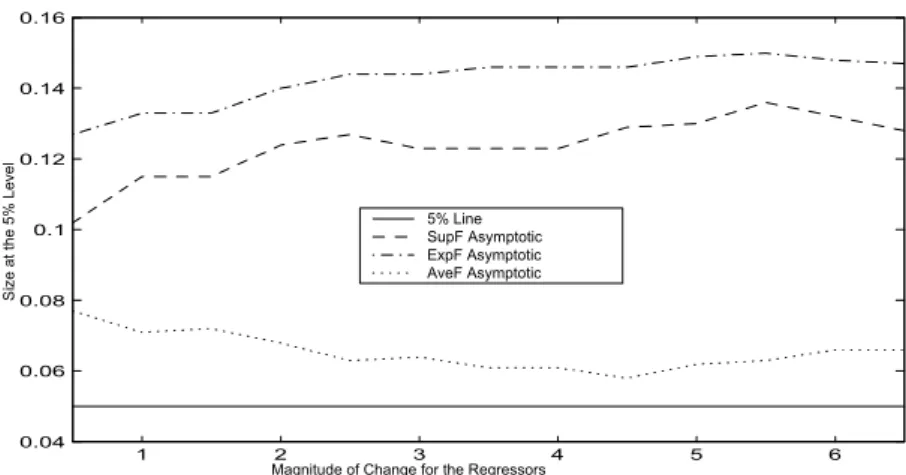
the most convenient and it may, in many circumstances, be the only method that is feasible. Figures1-2(Appendix A) show the PVFs constructed using the asymptotic distributions and for the case where there is a mean break in the regressors. They show the percentages of rejecting the null hypothesis at the5%level. In Figure1, we present the PVFs as function ofωfor_κ=T /2 = 20, and Figure2presents the ones as function of_κ forω = 3. We observe that theAveFT test is more accurate than the other tests especially theExpFT test which presents quite severe over-rejection in

(13)

the overwhelming majority of cases. Another feature of substantial importance is that the AveFT test performs quite well in the first case. However, the other tests are slightly more adequate in the second case in comparison with thefirst case. For the second case and unlike the AveFT test, the size distortions of theSupFT and ExpFT tests are severer when the break date is far from the boundaries of the sample.

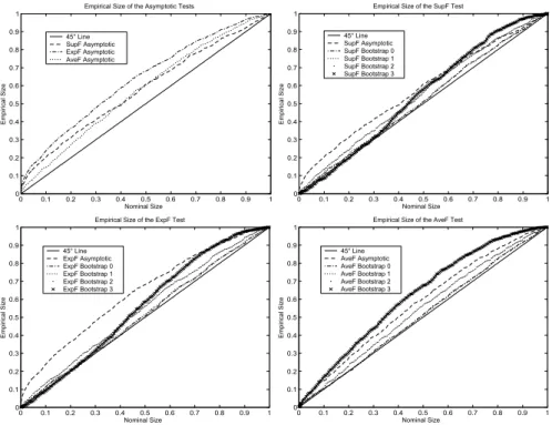
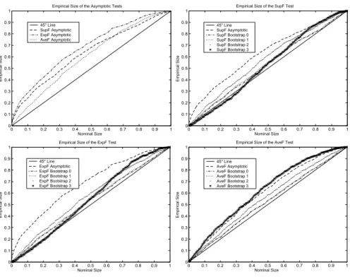
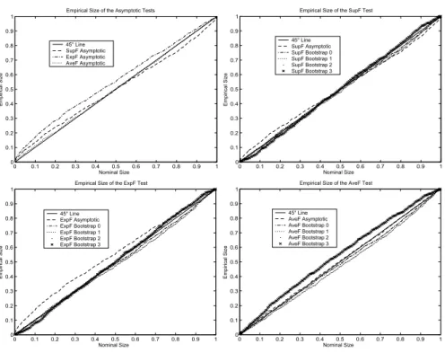
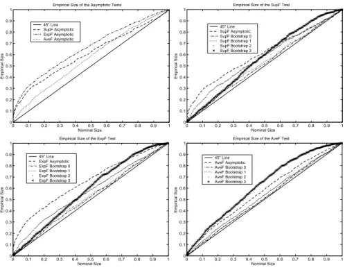
P value plots for the case whereω = 3and_κ=T /2 = 20are presented in Figures6-8(Appendix B). From the ones of tests based on the conventional asymptotic approximation, we first observe that the error in rejection probability committed by all the tests is severe especially when there is mean trend and mean break in the regressor process since the P value plots are above the45degree line, i.e. the actual size is greater than the nominal rejection frequency.22 This is not surprising since the asymptotic distributions of the test statistics have been derived under the hypothesis of stationary regressors. In comparison with the other tests, theExpFT test substantially over-reject more than the others, and the AveFT test is slightly more adequate than the SupFT test for the last regressor process.

Tests based on the Hansen’s bootstrap procedures are poor since they don’t allow to correct the size distortions of the asymptotic tests as they also over-reject relative to the nominal size. The heteroskedastic bootstrapAveFT test has higher tendency to over-reject than the one based on the conventional asymptotic approximation. This calls the usefulness and the validity of this bootstrap procedure into question. The parametric and nonparametric bootstrap procedures give similar results,23 correct the size distortions of the asymptotic tests and allow to do correct inference since the P value plots are very close to the 45 degree line, i.e. these tests achieve correct size. These procedures are then more accurate than the Hansen’s procedures which don’t completely solve the inference problem.

We now consider another case in which we set T = 50,δ2 = 0.50, δ3 = −0.75, and the other

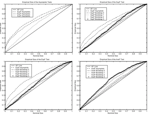
characteristics of the DGP are kept fixed. The P value plots are presented in Figures 9-11. We

first consider the tests based on the conventional asymptotic distribution. We observe that the SupFT test presents quite satisfactory results. The size distortions of the ExpFT test are quite severe especially when there is structural change in the regressor process. The AveFT test works well for thefirst two regressor processes since the P value plots are very close to the45degree line, i.e. the empirical size is very close to the correct rejection frequency. Thus, the error in rejection probability committed by this test is almost equal to zero (

¯ ¯ ¯Fˆ(αk)−αk ¯ ¯ ¯'0,_∀ k), which implies that the discrepancy P value plots are very close to the horizontal axisy= 0.

The bootstrapping versions of the SupFT test almost provide the same results as the con-ventional asymptotic distribution for the first two regressor processes. The performance of the heteroskedastic bootstrap is quite significantly poor when there is mean break in the regressors. The bootstrap procedures quasi-perfectly correct the size distortions of the asymptoticExpFT test

2 2_{This implies that} _F_ˆ₍_α

k)−αk > 0 for all k, which means that the discrepancy P value plots are above the

horizontal axisy= 0.

2 3_{This con}_fi_{rms the fact that the nonparametric bootstrap gives results indistinguishable from those of the}

para-metric bootstrap.

(14)

although there is slight under-rejection by the heteroskedastic bootstrap for the third regressor distribution. For the AveFT test, except for the heteroskedastic bootstrap which has tendency to over-reject, the other procedures are adequate. The parametric and nonparametric bootstrap procedures seem to be slightly more accurate than the Hansen’s procedures.

For the two considered cases, the theoretical results of Davidson and MacKinnon(1999)showing that the bootstrap tests should perform better are well proved for the parametric and nonparametric procedures. But, those showing that in many circumstances and in small samples, the bootstrap tests can show size distortions are well proved for the Hansen’s procedures in the overwhelming majority of cases.

From the obtained results of the two DGPs, we observe that there is diﬀerence in the results, and this may be explained by the fact that the performance of the tests may depend on how the data were actually generated. Thus, a test that works well against certain DGPs may not work well against others. This can be viewed in our Monte Carlo experiments for some testing procedures. 6.2. Inference when the null hypothesis is false

The anxiety for the size is understandable because a test with uncontrolled size is not useful regardless of the power. However, the fact that the bootstrap is able to eliminate the size distortions makes the test appropriate for a power study. In this case, we are interested in estimating the frequency of rejecting the null hypothesis when it is false. The main result in the analysis of power of the tests is found in Davidson and MacKinnon (2006). This result stipulates that the bootstrap tests with correct sizes can also often be shown to have the same power properties as their asymptotic counterparts. Consequently, if bootstrapping does result in a power loss whenB is large, that loss arises simply because bootstrapping corrects the tendency of the asymptotic tests to over-reject.

To compare the performance of the diﬀerent procedures we advocate the size-power curves constructed on the corrected size basis. We then require to carry out two experiences so as to generate Fˆ and Fˆ0 using the same sequence of random numbers to reduce the experimental error. Note that for the bootstrap tests, we don’t require to specify a priori the break date because the DGPs are constructed under the null hypothesis of no structural change.

Under the alternative hypothesis of structural change, the DGP is as follows:

yt= (

δ11+δ21yt−1+δ31yt−2+δ41xt−1+δ51xt−2+ut, 1≤t≤T /2, δ12+δ22yt−1+δ32yt−2+δ42xt−1+δ52xt−2+ut, T /2< t≤T,

(6.3) where T = 100 and ut ∼ i.i.d. N(0,1). The regression coeﬃcients are δ11 = 0.80, δ21 = 0.50,

δ31 = −0.75, δ41 = 1.00, δ51 = −0.50, δ12 = 0.30, δ22 = 0.00, δ32 = −0.25, δ42 = 0.50, and

δ52 = 0.00.24 The parametric and nonparametric bootstrap DGPs are then constructed using

the recursive rule given by (6.2) with the modification that in this case the regression coeﬃcient estimates (ˆδ1,ˆδ2,δˆ3,ˆδ4andˆδ5) are obtained under the incorrect assumption that the null hypothesis

2 4_{The magnitude of change}

θis then equal to0.50.

(15)

is true (see, section 4.5).25 We keep the same regressor processes considered in the study of the size performance.

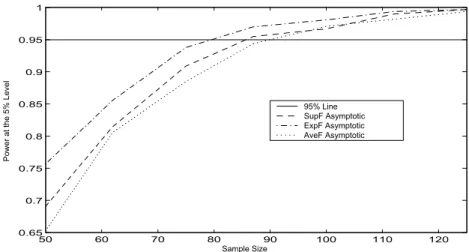
Figures3-5(Appendix A) show the PVFs constructed using the asymptotic distributions for all the regressor processes, respectively. They show the rejection proportions of the null hypothesis at the5%level as function of the sample size. Wefirst observe that the ExpFT test is more powerful than the others whatever the value of the sample size, and theSupFT test is in turn more powerful than theAveFT test except for the caseT = 100and the stationary regressor process. This power discrepancy between all the tests tends to zero as the sample size increases. Another feature of substantial importance is that the probability of rejecting the null hypothesis by all the tests tends to unity as the sample size increases.26 Thus, the tests areconsistent.

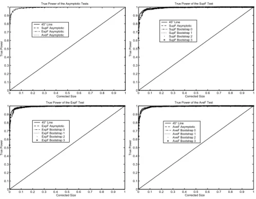
The size-power curves are presented in Figures12-14for the case whereω= 3and_κ=T /2 = 50. For all the tests, the procedures show perfect power properties for all the regressor processes with very slight superiority for the stationary distribution since the size-power curves are too close to the horizontal axis y = 1. The bootstrap tests don’t bring out any power loss since the intrinsic size-power curves are confused with those obtained for the asymptotic distribution. Thus, the theory that the test bootstrap power would be very similar to that of the asymptotic test on the basis of size correction is well proved.

The optimality properties of the ExpFT and AveFT tests obtained in large samples are main-tained under the conditions imposed here. The presence of mean trend and mean break in the marginal distribution of the regressors has not strongly aﬀected the results since almost the same power performance as for the stationary distribution is obtained.

The intuition often suggests that the bootstrap tests are less powerful than their asymptotic counterparts. This is because the formers have much less severe size distortions and then have low tendency to over-reject the null hypothesis unlike the asymptotic tests. The main result of this analysis is that in some cases, many bootstrap tests work very well since they have correct size and high power; property often diﬃcult to obtain when evaluating the performance of the tests in terms of size and power.

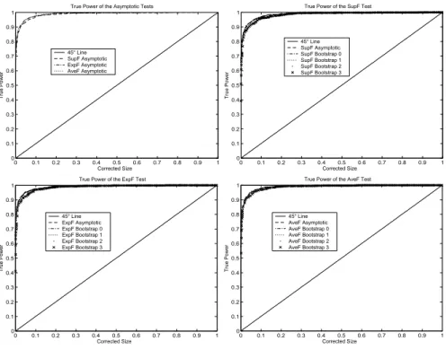
We now consider another DGP for which we setδ21= 0.90,δ31=−0.20,δ22= 0.40,δ32= 0.30,

and the other characteristics of the DGP are kept fixed. This is done to see whether the power performance of the tests depends on how the data are actually generated. The size-power curves are plotted in Figures15-17. In comparison with the results of the previous case, the procedures show lower power for all the regressor processes. As for thefirst DGP, there is very slight superiority for the stationary distribution since the corresponding size-power curves are closer to the horizontal axis y = 1 than those of the other regressor processes. The size-power curves of the bootstrap procedures are confused with those obtained for the asymptotic distribution. This proves once again the theory that the power of the bootstrap tests would be very similar to the one of the

2 5_{Note that}_ˆ_δ

1,ˆδ2,ˆδ3,ˆδ4 andˆδ5 cannot be consistent because when there exists a break date in the DGP while

the estimation is done without breaks, the obtained coeﬃcient regression estimates are not consistent because of the misspecification.

2 6_{This is obvious since as the intuition suggests, a test statistic having tendency to over-reject (section}₆_._{2) can}

have high power.

(16)

asymptotic tests on the corrected size basis. The results of this experiment show that change of some factors aﬀects the power performance of the tests, but globally it remains satisfactory.

The samples used in the applications are often larger than those used in our Monte Carlo experiments. However, all the procedures are accurate with a sample size of 100 in the cases considered here. Thus, there is not much to gain by carrying out experiments with larger sample sizes. To that eﬀect, we have carried out two other Monte Carlo experiments in which we set

|θ_|= 0.7 for the first andT = 150 for the second, and we kept fixed, for the two experiments, the other characteristics of the first considered DGP.27 The tests become more powerful for a larger magnitude of change. Thus, what is important to improve the power performance of the tests is the magnitude of jump and not the sample size.

6.3. Case of Student error terms

We now study the eﬀect of change of the error distribution on the performance of the testing procedures. To that eﬀect, we simulate leptokurtic data using the Student distribution with 5

degrees of freedom for the error terms. The same other characteristics of all the considered DGPs as well as the number of bootstrap and Monte Carlo replications are kept fixed. We claim that the number of bootstrap simulations,B = 999, is suﬃcient to capture the probability excess in the distribution tails.

For the study of the size performance, the P value plots are reported in Figures 18-20 for the

first DGP (model (6.1)) and in Figures 21-23 for the second DGP (model (6.1) with T = 50, δ2= 0.50 and δ3 =−0.75). We observe that there is a slight deterioration in the size performance

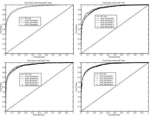
of the asymptotic tests for the two DGPs with respect to the Gaussian case. The correction of the size distortions by the parametric and nonparametric bootstrap procedures is quasi-perfect for the two DGPs as in the Gaussian case. The Hansen’s procedures show a slight degradation with respect to the Gaussian case for theSupFT andExpFT tests only for thefirst DGP. For the study of the power performance, the size-power curves are reported in Figures 24-26 for the first DGP (model(6.3)) and in Figures27-29 for the second DGP (model(6.3)withδ21= 0.90,δ31=−0.20,

δ22= 0.40andδ32= 0.30). The examination of these curves suggests that for the two DGPs, there

is a power loss with respect to the case of normal errors for all the testing procedures and whatever the regressor distribution.

We can then conclude that as the change of the DGP characteristics, the change of the error distribution aﬀects the size and power properties of the asymptotic and bootstrap testing procedures of single structural change.

7. Structural change analysis for U.S. interest rates

The importance of structural change in the U.S. inflation is considered by Ben Aïssaet al. (2004), Ben Aïssa and Jouini (2003), and Jouini and Boutahar (2003). Indeed, they use some selection procedures based on information criteria, sequence of tests for multiple breaks and a test similar

2 7

The results of these experiments are not reported here and are available upon request from the author.

(17)

to that based on Kolmogorov-Smirnov statistic applied to the evolutionary spectrum to determine the number of changes and their locations in the monthly U.S. inflation series. Both they find significant results since the breaks coincide with important facts and economic events such that the two Oil-Price Shocks and the major events in the International Monetary System.

The theory of the term structure of interest rates suggests that, if interest rates can be char-acterized asI(1)processes, then they should be cointegrated. Stock and Watson (1988) carry out cointegration tests for three monthly U.S. interest rates covering the period 1960:1-1979:8,28 and

find evidence of two cointegrating vectors. In the same context, Hansen(1992)tests the hypothesis that relationships between U.S. interest rates are stable over the period1960:1-1990:3. Indeed, he reports results of two fully modified regressions indicating that the change in the Federal Reserve’s operating procedures in 1979 altered the relationship between some interest rates. He finds that this regime-shift only appears to have aﬀected the relationship between the treasury-bill rates and the federal funds rate but not the relationship between the treasury-bill rates of diﬀerent maturities. 7.1. The modelling strategy and the results

In the same context of studying the relationship between U.S. interest rates, we propose a diﬀerent modelling strategy and apply the estimation and testing procedures discussed above using the monthly 90-day treasury-bill rate and the federal funds rate—plotted in Figure 30 (Appendix C)— covering the period 1957:1-2002:10 (yielding 550 observations) and obtained from the St. Louis Reserve Federal Bank database. Thus, we adopt a bivariate VAR(3)process:

yt=δ1+δ2yt−1+δ3yt−2+δ4yt−3+δ5xt−1+δ6xt−2+δ7xt−3+ut, (7.1)

whereyt is the 90-day treasury-bill rate andxtis the federal funds rate.

The number of bootstrap replications is set atB = 9999, a large value that we would recommend using in practice to improve the inference accuracy. The results of the diﬀerent testing procedures are as follows:

Asymptotic Bootstrap 0 Bootstrap 1 Bootstrap 2 Bootstrap 3

P value P value P value P value P value

SupFT 0.000 0.000 0.004 0.000 0.666

ExpFT 0.000 0.001 0.008 0.001 0.703

AveFT 0.165 0.169 0.156 0.132 0.376

The AveFT test fails to reject the null hypothesis of parameter stability for all the procedures even at the10%significance level. For the other tests, only the heteroskedastic bootstrap does not lead to reject the null hypothesis. The fact that this procedure does not allow a rejection of the null hypothesis is not surprising because the reported simulation results show that this procedure has sometimes tendency to under-reject the null hypothesis. However, the rejection of the null by

2 8_{They used data covering this period, presumably to exclude an eventual regime-shift in the term structure due}

to the change in the Federal Reserve’s operating procedures in1979.

(18)

the other procedures is obvious since the simulation results show that these procedures reject the null hypothesis with high proportions when there is a break in the data.

The relationship between the two series is then unstable and the break date thus selected by the SupFT test is located in 1981:5. Looking at the graphs of the series in Figure 30, we confirm the choice of this break since we observe that these series may be affected by structural breaks as there is a turbulence period at the beginning of the 1980s. The fact to find this regime-shift confirms the results of Hansen(1992)who found that the relationship between the 90-day treasury-bill rate and the federal funds rate has been affected by a regime-shift in1980. Thus, we see that with two different modelling strategies and two different techniques wefind the same regime-shift though the sample sizes are not the same. This gives us more information about the fact that the regime-shift is strongly evident and can be easily detected. The corresponding 95% confidence interval of the break date computed using the asymptotic distribution derived by Bai and Perron (1998) covers the quite large period stretching from1979:3to1984:2, indicating that the break date is imprecisely estimated.

The break date1981:5may be explained by the following events and facts. In1981, the United States of America have known the disinflation wave and which is known as "disinflation of Volcker" concerning a new control of the monetary policy. Indeed, before the year 1970, the repercussions of the real shocks on the economy were regarded as tiny. The considerablefluctuations of oil prices modified this point of view and led the Federal Reserve of the United States to reconsider the implementation of the monetary policy. In 1977, unemployment was running at 7%. Total labour costs to employers however, rose both in January1978and in 1979 because of increases in payroll taxes and the minimum wage, steps taken by administrative decision not market process but widely regarded as constituting almost as powerful an inflationary influence as were cash wage increases themselves. By 1979, spare capacity was becoming limited and production costs were rising at an annual rate of some 8%. During1979-1980, moreover, the price of oil and oil-related products also rose sharply under the spur of supply restrictions and rising world demand. In some ways the restrictive policies initially adopted to counter the stagflation of 1979-1980, like some of the main causes at work, followed lines similar to those observed in1974-1975. At a deeper level, however, the two sets of policies differed substantially. Couched primarily in terms of monetary aggregates, the post-1979policies seemed to embody a willingness to permit, and even to bring about, greater rises in interest rates than did the policiesfive years before, and the Federal Reserve’s discount rate at once edged up to 12%. After the election of Ronald Reagan in November 1980, the discount rates were raised to14%in May1981. The tax proposals of the president were totally different than the procedures taken in 1974-1975. President Reagan projected great tax cuts. The total effects of these last measures should lead to the restoration of the federal budget balance by 1984-1985. The year1981was marked by the rise of the tax deficit whereas the interest rates were on a rather high level of 9% and unemployment kept the margin of 8%. Actuated by the bad news coming from Mexico which had borrowed heavily and which stipulated that it doubts to refund its loans to the United States at the limits envisaged, all the American economy embarked on a productivity growth phase of the supported by a decrease of oil prices and the reduction of the inflation rate

(19)

of the with approximately 5%, but also by the deceleration of the raising of wages whereas the dollar, under the influence of the raised interest rates, attracted the flow of foreign capital, which appreciated approximately30%.

8. Conclusion

The paper has presented a detailed evaluation of the performance of some tests for single structural change based on the graphical methods of Davidson and MacKinnon (1998) whose interest is the principle of size correction that allows to show the true power of tests instead of the nominal power. The bootstrap methods improve the performance of the tests. The exception is that the Hansen’s heteroskedastic bootstrap has sometimes tendency to under-reject. Moreover, this procedure seems less precise than the asymptotic approximation for the AveFT test since the error in rejection probability committed by this bootstrapping version of the test is severer. The parametric and nonparametric bootstrap procedures are slightly more accurate than the hansen’s procedures. We found that on the basis of the corrected size, the bootstrap procedures have the same power properties than their asymptotic counterparts. The empirical illustration highlights the practical importance of the simulation results and indicates that the relationship between the interest rates has been altered by a regime-shift located at the beginning of the1980s.

Acknowledgements

The author is grateful to Emmanuel FLACHAIRE and the participants in the "Journées Doc-torales de l’ADRES", Paris, February 2005 for useful comments and remarks.

(20)

Appendix A: P value Functions 1 2 3 4 5 6 0.04 0.06 0.08 0.1 0.12 0.14 0.16

Magnitude of Change for the Regressors

S iz e at th e 5% L ev el 5% Line SupF Asymptotic ExpF Asymptotic AveF Asymptotic

Figure 1. Size of the Asymptotic Tests as Function of the Jump Size of the Regressors

5 10 15 20 25 30 35 40 45 0.04 0.06 0.08 0.1 0.12 0.14 0.16

Location of the Break for the Regressors

S iz e at th e 5 % L ev el 5% Line SupF Asymptotic ExpF Asymptotic AveF Asymptotic

Figure 2. Size of the Asymptotic Tests as Function of the Location of the Break for the

Regressors

(21)

50 60 70 80 90 100 110 120 0.65 0.7 0.75 0.8 0.85 0.9 0.95 1 Sample Size P ow er a t t he 5 % L ev el 95% Line SupF Asymptotic ExpF Asymptotic AveF Asymptotic

Figure 3. Power of the Asymptotic Tests as Function of the Sample Size for the Stationary

Regressor Process 50 60 70 80 90 100 110 120 0.6 0.65 0.7 0.75 0.8 0.85 0.9 0.95 1 Sample Size P ow er a t t he 5 % L ev el 95% Line SupF Asymptotic ExpF Asymptotic AveF Asymptotic

Figure 4. Power of the Asymptotic Tests as Function of the Sample Size for the Nonstationary

Regressor Process 50 60 70 80 90 100 110 120 0.55 0.6 0.65 0.7 0.75 0.8 0.85 0.9 0.95 1 Sample Size P ow er a t t he 5 % L ev el 95% Line SupF Asymptotic ExpF Asymptotic AveF Asymptotic

Figure 5. Power of the Asymptotic Tests as Function of the Sample Size for the Third Regressor

Process

(22)

Appendix B: P value Plots and Size-Power Curves 0 0.1 0.2 0.3 0.4 0.5 0.6 0.7 0.8 0.9 1 0 0.1 0.2 0.3 0.4 0.5 0.6 0.7 0.8 0.9 1 Nominal Size E m pi ric al S iz e

Empirical Size of the Asymptotic Tests 45° Line SupF Asymptotic ExpF Asymptotic AveF Asymptotic 0 0.1 0.2 0.3 0.4 0.5 0.6 0.7 0.8 0.9 1 0 0.1 0.2 0.3 0.4 0.5 0.6 0.7 0.8 0.9 1 Nominal Size E m pi ric al S iz e

Empirical Size of the SupF Test 45° Line SupF Asymptotic SupF Bootstrap 0 SupF Bootstrap 1 SupF Bootstrap 2 SupF Bootstrap 3 0 0.1 0.2 0.3 0.4 0.5 0.6 0.7 0.8 0.9 1 0 0.1 0.2 0.3 0.4 0.5 0.6 0.7 0.8 0.9 1 Nominal Size E m pi ric al S iz e

Empirical Size of the ExpF Test 45° Line ExpF Asymptotic ExpF Bootstrap 0 ExpF Bootstrap 1 ExpF Bootstrap 2 ExpF Bootstrap 3 0 0.1 0.2 0.3 0.4 0.5 0.6 0.7 0.8 0.9 1 0 0.1 0.2 0.3 0.4 0.5 0.6 0.7 0.8 0.9 1 Nominal Size E m pi ric al S iz e

Empirical Size of the AveF Test 45° Line AveF Asymptotic AveF Bootstrap 0 AveF Bootstrap 1 AveF Bootstrap 2 AveF Bootstrap 3

Figure 6. Empirical Size of the Tests for Stationary Regressor Process

0 0.1 0.2 0.3 0.4 0.5 0.6 0.7 0.8 0.9 1 0 0.1 0.2 0.3 0.4 0.5 0.6 0.7 0.8 0.9 1 Nominal Size E m pi ric al S iz e

Empirical Size of the ExpF Test 45° Line ExpF Asymptotic ExpF Bootstrap 0 ExpF Bootstrap 1 ExpF Bootstrap 2 ExpF Bootstrap 3 0 0.1 0.2 0.3 0.4 0.5 0.6 0.7 0.8 0.9 1 0 0.1 0.2 0.3 0.4 0.5 0.6 0.7 0.8 0.9 1 Nominal Size E m p iri ca l S iz e

Figure 7. Empirical Size of the Tests for Nonstationary Regressor Process

(23)

Figure 8. Empirical Size of the Tests when there is Mean Break in the Regressor Process

Empirical Size of the Asymptotic Tests

45° Line SupF Asymptotic ExpF Asymptotic AveF Asymptotic 0 0.1 0.2 0.3 0.4 0.5 0.6 0.7 0.8 0.9 1 0 0.1 0.2 0.3 0.4 0.5 0.6 0.7 0.8 0.9 1 Nominal Size E m pi ric al S iz e

Empirical Size of the SupF Test 45° Line SupF Asymptotic SupF bootstrap 0 SupF bootstrap 1 SupF bootstrap 2 SupF bootstrap 3 0 0.1 0.2 0.3 0.4 0.5 0.6 0.7 0.8 0.9 1 0 0.1 0.2 0.3 0.4 0.5 0.6 0.7 0.8 0.9 1 Nominal Size E m pi ric al S iz e

(24)

Empirical Size of the SupF Test 45° Line SupF Asymptotic SupF Bootstrap 0 SupF Bootstrap 1 SupF Bootstrap 2 SupF Bootstrap 3 0 0.1 0.2 0.3 0.4 0.5 0.6 0.7 0.8 0.9 1 0 0.1 0.2 0.3 0.4 0.5 0.6 0.7 0.8 0.9 1 Nominal Size Empirical Size of the ExpF Test

E m pi ric al S iz e 45° Line ExpF Asymptotic ExpF Bootstrap 0 ExpF Bootstrap 1 ExpF Bootstrap 2 ExpF Bootstrap 3 0 0.1 0.2 0.3 0.4 0.5 0.6 0.7 0.8 0.9 1 0 0.1 0.2 0.3 0.4 0.5 0.6 0.7 0.8 0.9 1 Nominal Size E m pi ric al S iz e

Figure 11. Empirical Size of the Tests when there is Mean Break in the Regressor Process

(25)

0 0.1 0.2 0.3 0.4 0.5 0.6 0.7 0.8 0.9 1 0 0.1 0.2 0.3 0.4 0.5 0.6 0.7 0.8 0.9 1 Corrected Size T ru e P ow er

True Power of the Asymptotic Tests

45° Line SupF Asymptotic ExpF Asymptotic AveF Asymptotic 0 0.1 0.2 0.3 0.4 0.5 0.6 0.7 0.8 0.9 1 0 0.1 0.2 0.3 0.4 0.5 0.6 0.7 0.8 0.9 1 Corrected Size T ru e P ow er

True Power of the SupF Test 45° Line SupF Asymptotic SupF Bootstrap 0 SupF Bootstrap 1 SupF Bootstrap 2 SupF Bootstrap 3 0 0.1 0.2 0.3 0.4 0.5 0.6 0.7 0.8 0.9 1 0 0.1 0.2 0.3 0.4 0.5 0.6 0.7 0.8 0.9 1 Corrected Size T ru e P ow er

True Power of the ExpF Test 45° Line ExpF Asymptotic ExpF Bootstrap 0 ExpF Bootstrap 1 ExpF Bootstrap 2 ExpF Bootstrap 3 0 0.1 0.2 0.3 0.4 0.5 0.6 0.7 0.8 0.9 1 0 0.1 0.2 0.3 0.4 0.5 0.6 0.7 0.8 0.9 1 Corrected Size T ru e P ow er

True Power of the AveF Test

45° Line AveF Asymptotic AveF Bootstrap 0 AveF Bootstrap 1 AveF Bootstrap 2 AveF Bootstrap 3

Figure 12. True Power of the Tests for Stationary Regressor Process

True Power of the SupF Test

45° Line SupF Asymptotic SupF Bootstrap 0 SupF Bootstrap 1 SupF Bootstrap 2 SupF Bootstrap 3 0 0.1 0.2 0.3 0.4 0.5 0.6 0.7 0.8 0.9 1 0 0.1 0.2 0.3 0.4 0.5 0.6 0.7 0.8 0.9 1 Corrected Size T ru e P ow er

True Power of the ExpF Test

45° Line ExpF Asymptotic ExpF Bootstrap 0 ExpF Bootstrap 1 ExpF Bootstrap 2 ExpF Bootstrap 3 0 0.1 0.2 0.3 0.4 0.5 0.6 0.7 0.8 0.9 1 0 0.1 0.2 0.3 0.4 0.5 0.6 0.7 0.8 0.9 1 Corrected Size T ru e P ow er

Figure 13. True Power of the Tests for Nonstationary Regressor Process

(26)

True Power of the SupF Test 45° Line SupF Asymptotic SupF Bootstrap 0 SupF Bootstrap 1 SupF Bootstrap 2 SupF Bootstrap 3 0 0.1 0.2 0.3 0.4 0.5 0.6 0.7 0.8 0.9 1 0 0.1 0.2 0.3 0.4 0.5 0.6 0.7 0.8 0.9 1 Corrected Size T ru e P ow er

Figure 14. True Power of the Tests when there is Mean Break in the Regressor Process

Figure 15. True Power of the Tests for Stationary Regressor Process

(27)

Figure 16. True Power of the Tests for Nonstationary Regressor Process

0 0.1 0.2 0.3 0.4 0.5 0.6 0.7 0.8 0.9 1 0 0.1 0.2 0.3 0.4 0.5 0.6 0.7 0.8 0.9

1 True Power of the Asymptotic Tests

Corrected Size T ru e P ow er 45° Line SupF Asymptotic ExpF Asymptotic AveF Asymptotic 0 0.1 0.2 0.3 0.4 0.5 0.6 0.7 0.8 0.9 1 0 0.1 0.2 0.3 0.4 0.5 0.6 0.7 0.8 0.9 1 Corrected Size T ru e P ow er

Figure 17. True Power of the Tests when there is Mean Break in the Regressor Process

(28)

0 0.1 0.2 0.3 0.4 0.5 0.6 0.7 0.8 0.9 1 0 0.1 0.2 0.3 0.4 0.5 0.6 0.7 0.8 0.9

1 Empirical Size of the Asymptotic Tests

Nominal Size E m pi ric al S iz e 45° Line SupF Asymptotic ExpF Asymptotic AveF Asymptotic 0 0.1 0.2 0.3 0.4 0.5 0.6 0.7 0.8 0.9 1 0 0.1 0.2 0.3 0.4 0.5 0.6 0.7 0.8 0.9

1 Empirical Size of the SupF Test

Nominal Size E m pi ric al S iz e 45° Line SupF Asymptotic SupF Bootstrap 0 SupF Bootstrap 1 SupF Bootstrap 2 SupF Bootstrap 3 0 0.1 0.2 0.3 0.4 0.5 0.6 0.7 0.8 0.9 1 0 0.1 0.2 0.3 0.4 0.5 0.6 0.7 0.8 0.9

1 Empirical Size of the ExpF Test

Nominal Size E m pi ric al S iz e 45° Line ExpF Asymptotic ExpF Bootstrap 0 ExpF Bootstrap 1 ExpF Bootstrap 2 ExpF Bootstrap 3 0 0.1 0.2 0.3 0.4 0.5 0.6 0.7 0.8 0.9 1 0 0.1 0.2 0.3 0.4 0.5 0.6 0.7 0.8 0.9 1 Nominal Size E m pi ric al S iz e

Empirical Size of the Asymptotic Tests 45° Line SupF Asymptotic ExpF Asymptotic AveF Asymptotic 0 0.1 0.2 0.3 0.4 0.5 0.6 0.7 0.8 0.9 1 0 0.1 0.2 0.3 0.4 0.5 0.6 0.7 0.8 0.9

1 Empirical Size of the SupF Test

Nominal Size E m pi ric al S iz e 45° Line SupF Asymptotic SupF Bootstrap 0 SupF Bootstrap 1 SupF Bootstrap 2 SupF Bootstrap 3 0 0.1 0.2 0.3 0.4 0.5 0.6 0.7 0.8 0.9 1 0 0.1 0.2 0.3 0.4 0.5 0.6 0.7 0.8 0.9 1 Nominal Size E m pi ric al S iz e