Ratio plot and ratio regression
with applications to social and
medical sciences
Dankmar B¨ohning
Southampton Statistical Sciences Research Institute & Mathematical Sciences, University of Southampton
Abstract. We consider count data modeling, in particular, the zero-truncated case as it arises naturally in capture-recapture modeling as the marginal distribution of the count of identifications of the members of a target population. Whereas in wildlife ecology these distributions are often of a well-defined type, this is less the case for social and medical science applications since study types are often entirely ob-servational. Hence, in these applications, violations of the assumptions underlying closed capture-recapture are more likely to occur than in carefully designed capture-recapture experiments. In consequence, the marginal count distribution might be rather complex. The purpose of this note is to sketch some of the major ideas in the recent developments in ratio plotting and ratio regression designed to explore the pattern of the distribution underlying the capture process. Ratio plotting and ratio regression are based upon considering the ratios of neighboring probabilities which can be estimated by ratios of observed frequencies. Frequently, these ratios show patterns which can be easily modeled by a regression model. The fitted regression model is then used to predict the frequency of hidden zero counts. Particular attention is given to re-gression models corresponding to the negative-binomial, multiplicative binomial and the Conway-Maxwell-Poisson distribution.
Key words and phrases: closed capture-recapture, Conway-Maxwell-Poisson, mixtures, multiplicative-binomial, negative-binomial, zero-truncated count distributions.
1. INTRODUCTION
We are interested in zero-truncated count distributional modelling which arises naturally in capture-recapture experiments or studies. The size N of a target population needs to be determined. For this purpose a trapping experiment or study is done where members of the target population are identified at T oc-casions where T might be known or not. Furthermore, the sampling occasions Dankmar B¨ohning is Professor in Medical Statistics, Southampton Statistical Sciences Research Institute, University of Southampton, Southampton, SO17 1BJ, UK (e-mail: d.a.bohning@soton.ac.uk)
∗
The author is grateful to all editors and reviewers for the many helpful comments. 1
might be specified prior to the study or they might occur randomly during the observational period. For each member i the count of identifications Xi is
re-turned where Xi takes values in {0,1,2,· · · } for i = 1,· · ·, N. However,
zero-identifications are not observed; they remain hidden in the study. Hence, a zero– truncated sample X1,· · · , Xn is observed, where we have assumed w.l.o.g. that
Xn+1 = · · · = XN = 0. So, n is the number of recorded individuals. The
as-sociated untruncated and zero-truncated densities will be denoted as px(θ) and
p+x(θ) = px(θ)/[1−p0(θ)], respectively. The setting above has been developed
primarily for wildlife populations (Bunge and Fitzpatrick 1993, Borchers et al. 2004, Chao 2001, Sanathanan 1977, Wilson and Collins 1992). We are interested here to apply the framework to social and medical scenarios as we will illustrate in the following three examples.
1.1 Homeless population of the city of Utrecht
As illustration of the problem, we consider the question of estimating the home-less population of Utrecht (NL). The city of Utrecht runs a shelter where homehome-less people can stay overnight. Data are available for a period of 14 nights in 2013 and are shown in Table1. It can be assumed that the shelter covers only the city of Utrecht. The table contains information on how often homeless people stayed in the shelter within this 14-nights period. For example, f1 = 36 people stayed
exactly one night, whereasf2 = 11 people stayed exactly two nights, and so forth.
In total, 222 different homeless people stayed in the shelter, spending a total of
S =P14
x=1xfx = 2,009 nights there. For more details see van der Heijden et al.
(2014a). In this case, the number of occasions is known with T = 14 and also the occasions are specified in the observational period. Whereas some homeless people use the shelter frequently, others use it only occasionally or very rarely. Hence the register for homeless people based on the shelter is incomplete. The city of Utrecht is interested in the total size of its homeless population. Hence, we are interested to find an estimate ofN, or, equivalently, off0, the size of the
hidden homeless population.
Table 1
Frequency distribution of the number of nightsxstayed in the shelter per homeless person for
the city of Utrecht for a period of 14 nights in 2013
x 1 2 3 4 5 6 7 8 9 10 11 12 13 14 n fx 36 11 6 11 5 7 6 11 3 8 7 12 22 77 222
1.2 Domestic violence in NL
In a study of domestic violence, van der Heijden et al. (2014b) reports per-petrator offense data in the Netherlands for the year 2009. The data represent the Netherlands excluding the police region for The Hague. Here the perpetrator study is reported in Table 2. In this case T is unknown and there are no pre-specified sampling occasions as domestic violence incidents occurred at unplanned time points in the observational period 2009.
Table 2
Frequencies of the number of times perpetrators have been identified in a domestic violence incident in the Netherlands in the year 2009
x 1 2 3 4 5 6 7 8 9 n fx 15,169 1,957 393 99 28 8 6 1 1 17,662
There were 15,169 perpetrators identified as being involved in a domestic vio-lence incident exactly once, 1,957 exactly twice, and so forth. In total, there were 17,662 different perpetrators identified by the police in the Netherlands for 2009. As not every case of domestic violence is reported to the police, an unknown number of perpetrators remain hidden. Hence, here the target population of in-terest consists of the perpetrators in the Netherlands (excluding The Hague) in the year 2009, whether they have been identified by the police or not.
1.3 Size of forced labour worldwide
The International Labour Office (ILO) undertook a study to estimate the size of forced labour worldwide (ILO 2012). Here forced labour is characterized by provision of some form of work or service which is done under threat of penalty and undertaken involuntarily. Frequently the term slave labour is used instead (Bales 2012). Due to its hidden nature forced labour is hard to measure. For this reason, the ILO launched a capture-recapture study to estimate the size of forced labour worldwide. Teams were established and searched for reports on forced labour. Sources of information included media, government reports, academic and trade union reports and many more. In total about 2500 different sources have been used. The period that was covered was the years 2002 – 2011. Reports were collected from anywhere in the world and therefore considerable heterogeneity should be expected. Table 3 shows the zero-truncated frequency distribution of the count x, the number of times a case of forced labour has been identified in any of the sources. There were 4069 cases of forced labour that were exactly identified by 1 report, 1,186 cases that were identified by 2 different reports etc. Each case will have a certain number of persons involved. From this an estimate of the size of forced labour (the number of people involved) can be derived. Here we are interested in estimating the number of cases f0 that were identified by x= 0 reports.
Table 3
Frequency distribution of forced labour report counts
x 1 2 3 4 5 6 7 8 9 10 11 n
fx 4,069 1,186 167 46 10 7 3 1 0 1 1 5,491
1.4 Screening for bowel cancer
Bowel cancer can develop without any early warning signs. The Faecal Occult Blood Test (FOBT) can detect small amounts of blood in the bowel motion. This might be indicative of a problem such as cancer but also something else such as polyps or nothing at all. Lloyd and Frommer (2008, 2004a, 2004b) present results of a screening study for bowel cancer in Sydney (Australia). From 1984 onwards about 50000 subjects were screened for bowel cancer using the FOBT. Self-administered testing took place onT = 6 successive days and at each of the
6 occasions absence or presence of blood in faeces was recorded. If at least one of theT tests is positive a gold standard evaluation took place and results could be healthy, polyps, or cancer. A person that tested negatively on all T tests is not further assessed. Out of exactly 49,927 persons, 46,553 tested negatively on all six tests (and these were not further investigated). Out of the other 3374 subjects who tested positively at least once, 3106 were examined and their true disease status determined. The other 268 subjects who tested positively were lost to the study. In Table4we see the frequency distribution of the 228 persons with cancer where x is the count of positive tests in the 6-days period. As 46,553 remained without further assessment the question arises of how much hidden cancer is present among this unassessed population.
Table 4
Frequency distribution of number of positive tests of those with cancer and testing positive at least once (Lloyd and Frommer 2008)
x 1 2 3 4 5 6 n fx 46 27 26 33 39 57 228
1.5 Assumptions involved in the ratio-regression approach
The ratio-regression approach to be presented is not assumption-free. We as-sume that the target population is closed, e. g. that there is no migration, no deaths, and no births. Specifically, the no-migration assumption can be question-able in some of the examples above such as the homeless study in the city of Utrecht. Here, the size of the time window is a steering element in satisfying the closed-population assumption. The larger the observational period the more likely is the occurrence of migration. The smaller the period the less homeless people are observed. In this case, it was found that 14 days established a reasonable compromise as increasing the period by one week did not add substantially more homeless people to the observed part of the homeless population. An alternative way to proceed would be to use open population modeling such as the Cormack-Jolly-Seber model (McCrea and Morgan 2015; see also Cormack 1964, Jolly 1965, Seber 1965 and this special issue) in which the time-specific dependency of the data is incorporated.
In some cases it might be unclear how the target population is defined. Whereas in the case of the bowel cancer study1.4the target population is thedisease-free screened population, this is less clear in the domestic violence study 1.2 of the Netherlands. Here, we define the target population to be all perpetrators that actually performed acts of domestic violence whether this has been identified by the authorities or not.
2. RATIO PLOT
We aim to estimate the population sizeN. AsN =N p0+N(1−p0) wherep0 is
the probability of a zero count or missing an observation, we can get an estimate of N by using the moment estimate n forN(1−p0) and solving ˆN = ˆN p0+n
for ˆN = n/(1−p0), a Horvitz-Thompson estimate of N. As p0 is unknown
in most applications (and certainly in those of section 1) we need to come up with some estimate for p0. A natural way to proceed is to use a parametric
p+x(θ) for x = 1,2,· · · , and use ˆθ in p0(ˆθ) to estimate N. See also Sanathanan
(1977). McCrea and Morgan (2015) call ˆN =n/[1−p0(ˆθ)] a
Horvitz-Thompson-like estimate to distinguish it from the conventional Horvitz-Thompson estimate ˆ
N =n/(1−p0).
A natural starting point for searching for an appropriate count distribution is the power series density
(1) px(θ) =axθx/η(θ)
where ax is a known, nonnegative coefficient, θ a positive parameter and x =
0,1,· · · ranges over the set of nonnegative integers. Also, η(θ) = P∞
x=0axθx
is the normalizing constant. The power series distribution contains the Poisson (ax= 1/x!), the binomial (ax= Txforx= 0,· · · , T with positive integerT and
ax = 0 for x > T) or the geometric (ax = 1).
5 4 3 2 1 0 1.0 0.8 0.6 0.4 0.2 0.0 count x p 0.4 6 5 4 3 2 1 0 35000 30000 25000 20000 15000 10000 5000 0 count x freq uenc y
Fig 1. Ratio plot for a sample of 100,000 counts from a binomial withT= 6and event parameter
p= 0.4(left panel) and frequency distribution (right panel). The vertical axis in the left panel
showspˆ= ˆrx/(1 + ˆrx).
It is a fundamental property of the power series distribution that
(2) rx= px+1(θ)/ax+1 px(θ)/ax = p + x+1(θ)/ax+1 p+x(θ)/ax =θ,
the ratio of neighboring probabilities multiplied by the inverse of their respective coefficients is a constant, independent ofx, in fact it is the parameterθitself. This property occurs for the untruncated as well as for the zero-truncated distribution as the normalizing constant (1−p0(θ)) cancels out. The quantityrx can be used
to develop adiagnostic devicefor the presence of a particular distribution. Aspx
is an unknown quantity we replace it by its nonparametric estimatefx/N so that
we obtain an empirical ratio
(3) rˆx = ax ax+1 fx+1 fx ,
as the unknown quantity N cancels out. Plotting ˆrx against x provides the
em-pirical ratio plot or simply the ratio plot. If the ratio plot shows a horizontal line pattern we can take this as supportive evidence for the presence of the dis-tribution of interest. The determining quantity in (3) is the ratio ax/ax+1 of
the coefficients of the power series family member. For the Poisson this ratio is
ax/ax+1 =x+ 1, for the binomial it is ax/ax+1 = (x+ 1)/(T −x), and for the
geometric it is simplyax/ax+1 = 1. As the ratio plot construction depends on the
coefficientax we emphasize this by mentioning the family member. For example,
if we use the concept for the binomial we speak of thebinomial ratio plot, if we use it for the geometric we speak of thegeometricratio plot. If there is no doubt of which family member is used we simply speak about the ratio plot. The ratio plot has been developed in its basic form in B¨ohning et al. (2013). We illustrate the concept for the binomial in Figure1. 100,000 counts have been sampled from a binomial with size parameterT = 6 and event parameterp= 0.4 corresponding to the parameterization in the power series of θ = p/(1−p) = 2/3. In the left panel of Figure 1 we see the ratio plot for the binomial on the event parameter scale. There is clear evidence of a horizontal line pattern supporting the binomial distribution. The benefit of the diagnostic device becomes clear when comparing it to the bar chart provided in the right panel of Figure 1 where the binomial distribution is more difficult to recognize.
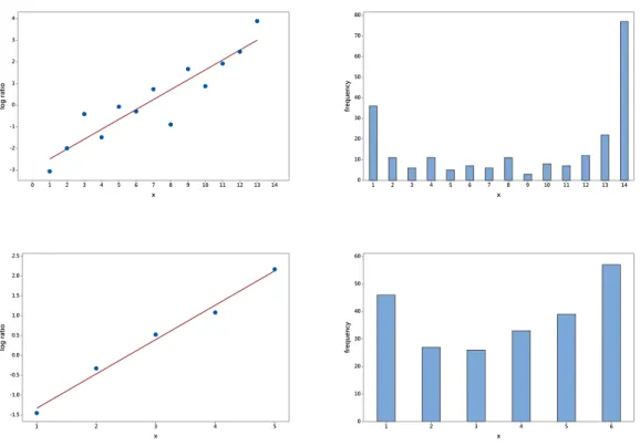
14 13 12 11 10 9 8 7 6 5 4 3 2 1 0 4 3 2 1 0 -1 -2 -3 x log ratio 14 13 12 11 10 9 8 7 6 5 4 3 2 1 80 70 60 50 40 30 20 10 0 x freq uenc y 5 4 3 2 1 2.5 2.0 1.5 1.0 0.5 0.0 -0.5 -1.0 -1.5 x log ratio 6 5 4 3 2 1 60 50 40 30 20 10 0 x freq uenc y
Fig 2. Binomial ratio plot (on the log-scale) for homeless data of section1.1 (upper left panel)
and bowel cancer data of section 1.4 (lower left panel) with associated frequency distributions
(upper and lower respective right panel)
We now apply the binomial ratio plot to the homeless study data of section
1.1 and the bowel cancer data of section 1.4. Figure 2 shows the ratio plot for the homeless data of Utrecht (upper left panel) and for the bowel cancer data (lower left panel). Note that the ratio ˆrx = (x+ 1)/(T−x)×fx+1/fx is plotted
on the log-scale. The associated frequency distributions are provided in the right panels of Figure2. There is clear evidence that a horizontal line pattern does not
hold. There could be various reasons why a horizontal line pattern is violated in the ratio plots present in Figure 2. It could be that the repeated visits to the homeless shelter (upper left panel) are not independent or that homeless people have different tendencies to visit the shelter. Similar issues might occur in the bowel cancer data (lower left panel) where repeated testing might not be independent or different patients might have different risk for a positive test. An alternative approach to deal with dependencies between occasions is the approach using log-linear models as suggested by Fienberg (1972) and Cormack (1989). See also Chao (2001). This approach requires availability of the data in form of complete capture histories xij where xij = 1 if unit iis identified at occasion j
and 0 otherwise. In certain applications such as the homeless or bowel cancer data occasion-specific data might be available (although we did not have access to these for the present work), in other applications such as the worldwide forced labour study only xi =PTj=1xij is available and log-linear modelling is not possible in
these cases.
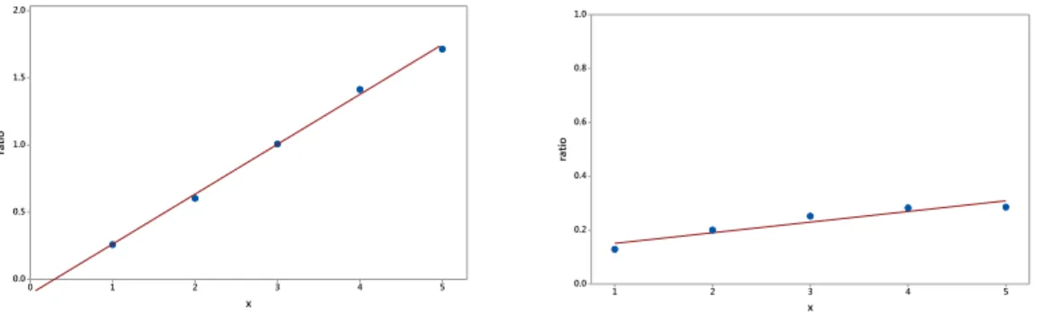
Let us now turn to the domestic violence data of section 1.2. The Poisson ratio plot in Figure3(left panel) provides evidence for a violation of the Poisson assumption in this case. There is a clear positive trend visible in the ratio plot. However, there is no reason why we can expect domestic violence counts to follow a Poisson distribution. We might as well consider the geometric distribution and its associated ratio plot implying plottingx →fx+1/fx as provided in the right
panel of Figure3. Apparently, there is also a positive trend visible although this appears more diminished in the geometric ratio plot than in the Poisson ratio plot. We denote by T0 the largest count considered, in this case T0 = 5. Note
that T0 ≤ T if the number of sampling occasions is known. An inspection of
the chi-square goodness-of-fit statistic χ2 = PT0−1
x=1 (log ˆrx−log ¯rx)2/vard(log ˆrx)
confirms this impression. Here, vard(log ˆrx) = 1/fx+1 + 1/fx (Rocchetti et al.
(2011), B¨ohning et al. (2013)), and for estimating the parameter θ we use the consistent and asymptotically unbiased estimates ¯rx =PxT=10−1(x+ 1)fx+1/fx for
the Poisson ratio plot and ¯rx = PTx=10−1fx+1/fx for the geometric Poisson ratio
plot. We find χ2 = 382.54 for the Poisson and χ2 = 94.86 for the geometric ratio plot, both withT0−1 = 4 df. Thus, it is clear that even in the case of the
geometric the fit is not yet acceptable, and we will turn to ratio regression in the next section to extend the modelling framework considerably.
3. RATIO REGRESSION
The basic idea is to extend the ratio plot to a full regression approach. Consider ˆ
rx = axax+1fxf+1x and the regression model in count x
(4) ˆrx=
p
X
j=1
βjgj(x)
where gj(x) is a known regression function of count x. In most applications we
have in mind, p= 2 orp= 3, and gj(x) is of simple structure such asg1(x) = 1
and g2(x) =x org2(x) = log(x+ 1). After estimating the coefficients β1,· · · , βp
we can estimatef0 as (5) fˆ0 = a0 a1 f1 Pp j=1βˆjgj(0) .
5 4 3 2 1 0 2.0 1.5 1.0 0.5 0.0 x ra tio 5 4 3 2 1 1.0 0.8 0.6 0.4 0.2 0.0 x rati o
Fig 3. Poisson ratio plot (left panel) and geometric ratio plot (right panel) for the domestic
violence data of the Netherlands ignoring low frequency datax≥6
3.1 Ratio regression and mixtures
We are interested in connecting the presence of unobserved heterogeneity (which could be described by a latent variable) with the concept of the ratio plot and ratio regression. If the target population consists of subpopulations and subpopulation membership is not observed we speak of the occurrence of unob-served heterogeneity. For example, in the case study on forced labour1.3, reports were collected from anywhere in the world and therefore considerable hetero-geneity should be expected. Assuming that in each subpopulation a power series distribution is valid then unobserved heterogeneity leads to a mixture of power series distributions mx =
R
θpx(θ)f(θ)dθ, where f(θ) represents the mixing
dis-tribution, the distribution of the subpopulation parameter θ in the population. Hence mixtures of parametric count distributions have attracted some attention in capture-recapture modelling (Dorazio and Royle 2005, Pledger 2005, Norris and Pollock 1996, Wang and Lindsay 2005, 2008, Mao and You 2009, B¨ohning and Kuhnert 2006). We can likewise consider the ratio plot for mixtures
(6) rx =
ax
ax+1 mx+1
mx
where we use again the known coefficientsax associated with the mixture kernel,
for example, in the case of a Poisson kernelax= 1/x! or the case of a geometric
kernelax= 1. The estimate ofrx will not change; however, the interpretation of
the observed pattern in the ratio plot will. This is mainly due to the following result (B¨ohning and Del Rio Vilas 2008):
Theorem1. Let mx=
R
θpx(θ)f(θ)dθ where px(θ)is a member of the power
series family and f(θ) an arbitrary density. Then, for rx = aax+1x mmx+1x we have
the following monotonicity:
rx≤rx+1
for allx= 0,1,· · ·.
The result in Theorem 1 can be interpreted as saying that the presence of unobserved heterogeneity will force a monotone increasing pattern in the ratio plot. In some special cases for the mixing distribution stronger results are possible.
Suppose thatX|Θ=θ is Poisson with densitypx(θ) and suppose further that the
density f(θ) of Θ is a gamma with parameters k and β. Then, using standard knowledge, mx= Rθpx(θ)f(θ)dθ= Γ(k1)βk R∞ 0 exp(−θ)θx x! ×θk −1exp(−θ/β)dθ = Γ(Γ(x+1)Γ(x+k)k)β−kβ+1β k+x, (7)
which corresponds to a negative-binomial with parameterp= 1/(β+ 1) so that
(8) mx =
Γ(x+k)
Γ(x+ 1)Γ(k)(1−p)
xpk.
It is easy to work out thatrx= aaxx+1mmx+1x = (x+ 1)mmx+1x = (1−p)(x+k) in this
case, so that the monotone pattern in the ratio plot becomes a straight line with intercept (1−p)kand positive slope (1−p).
3.2 Ratio regression and Chao estimation
Another question is how the result in Theorem 1connects to established esti-mators such as Chao’s estimator (Chao 1987, 1989). Chao’s estimator of f0 has
been developed as a lower bound estimator under mx = Rθpx(θ)f(θ)dθ where
px(θ) is the Poisson density and f(θ) an arbitrary mixing distribution. The
orig-inal estimator takes the form ˆf0 = f12/(2f2) and is one of the most frequently
used estimators in capture-recapture modeling.
We letpx(θ) be any member of the power series now. Then Theorem1 implies
(9) a0 a1 m1 m0 ≤ ax ax+1 mx+1 mx forx= 0,1,· · ·.
For x = 1 it follows that m0 ≥ (a0a2/a12)(m21/m2), and replacing mx by fx/N
leads to Chao’s lower bound estimator (a0a2/a21)(f12/f2) for f0 in the case of
the power series family, and in particular to f12/(2f2) in the Poisson case. The
lower bound estimator becomes asymptotically unbiased if there is no heterogene-ity (the mixing distribution becomes a one mass point distribution). Note that the lower bound estimator is valid for any mixing distribution on θ including a discrete mixing distribution with point mass at zero (leading to a zero-inflated distribution) as this is a special case of a discrete mixing distribution. However, its bias will depend on the choice of the mixture kernel. For example, in the case of the domestic violence data of section1.2we can expect, by inspecting the ratio plot in Figure 3, that the geometric lower bound will have a smaller bias than the Poisson lower bound as the bias-determining difference
(10) a0 a1 f1 f0 −a1 a2 f2 f1
can be expected to be smaller for the geometric than for the Poisson.
The result of Theorem 1 allows many lower bound estimators since m0 ≥
(a0ax+1/ax) (m1mx/mx+1) for x = 1,2,· · ·. For example, (a0a3/a2)(f1f2/f3)
provides a lower bound estimator forf0 if we choose x = 2. However, none will
be as sharp as Chao’s lower bound, the one we obtain for x = 1. Nevertheless, considering the ratios rx for x > 1 can be helpful and ratio regression can be
3.3 Ratio regression and empirical Bayes
The ratiorx = axax+1mmx+1x has an interesting connection to Bayesian inference.
In fact, rx = aax+1x mmx+1x = axax+1 R θax+1θ x+1/η(θ)f(θ)dθ R θaxθ x/η(θ)f(θ)dθ = R θθ× axθx/η(θ)f(θ) R θaxθ x/η(θ)f(θ)dθdθ= R θθf(θ|x)dθ (11)
is the posterior mean w.r.t. the prior distribution f(θ) on θ. Here f(θ|x) =
axθx/η(θ)f(θ)
R
θaxθ
x/η(θ)f(θ)dθ is the posterior distribution. Hence ˆrx =
ax
ax+1
fx+1
fx provides an
estimate of the posterior meanwithout assuming any knowledge of the prior dis-tribution nor is there any requirement for estimating the prior disdis-tribution, an idea which goes back to Robbins (1955) and is considered the origin of empir-ical Bayes. For more details see Carlin and Louis (2011). In conclusion, when modellingrx we are modelling the posterior mean.
3.4 Ratio regression and count distribution modeling
We return to the ratio regression approach (4). To ensure positive fitted values we need to incorporate a link-function leading to the ratio-regression model
(12) log ˆrx =
p
X
j=1
βjgj(x)
where gj(x) is a known regression function of count x. Indeed, fitting a simple
straight line to ˆrxin the domestic violence data of section1.2would lead to a
neg-ative intercept estimate (see left panel of Figure3) and, hence, to a non-feasible estimate off0. This is not a specific problem of the least-squares estimation
tech-nique used here, but a more general deficiency of the negative-binomial as also the maximum likelihood estimate of the shape parameter lies on the boundary of the parameter space. Invoking an appropriate link-function such as the log-link avoids this non-feasibility, but we are also losing the interpretation of the straight line ratio regression as the negative-binomial model. Instead of working with the negative-binomial we can try the Conway-Maxwell-Poisson distribution given by
(13) mx=
1
C θx
(x!)ν,
forx= 0,1,· · · and positiveθandν. The normalizing constantC=P∞
x=0θx/(x!)ν
is not available in closed form. For more details see Sellers and Shmueli (2010). It is easy to see thatrx= (x+ 1)mx+1/mx =θ(x+ 1)1−ν which suggests the ratio
regression approach with log-link
(14) logrx =β1+β2log(x+ 1)
whereβ1= logθandβ2 = (1−ν) and the restrictionβ2≤1. Hence working with
the Conway-Maxwell-Poisson distribution is equivalent to working with a straight line model on the log-scale for the ratio regression. We see the log[(x+ 1)fx+1/fx]
and the model fit for β1 +β2log(x+ 1) in Figure 4 for the domestic violence
5 4 3 2 1 1.0 0.5 0.0 -0.5 -1.0 -1.5 x log ratio observed b1+b2 log(x+1) b1 + b2 log(x+1)+b3 x
Fig 4. Poisson ratio regression usingβ1+β2log(x+ 1)(solid curve) andβ1+β2log(x+ 1) +β3x
(dashed curve) for the domestic violence data of section1.2
good for x = 1,2,3, it is deteriorating for values x = 4,5. The model logrx =
β1 +β2log(x+ 1) +β3x provides an excellent fit for all x−values as Figure 4
shows. An estimate ˆf0 is simply found from the estimated regression coefficients
as ˆf0 =f1exp(−βˆ1). Here as well as for the general case of the modelE(Y) =Xβ,
we use the weighted least-squares estimate
(15) βˆ= (XTWX)−1XTWY,
whereY = (logr1,· · ·,logrT0−1)
T,X is the design matrix containing the
regres-sion functions of the model, W is a diagonal matrix containing the estimated inverse variances of Y1,· · ·, YT0−1, more precisely, wi = (1/fi+ 1/fi+1)
−1. Here T0 is the largest count considered. Note that the estimated covariance matrix of
(15) is readily available as
(16) covd(βˆ) = (X
TWX)−1.
The ratio regression approach opens the door to a huge arena of techniques. However, whatever we choose as regression model we would like to make sure to include an intercept term as this guarantees that the power series family is included as a special case. For example, in the Poisson ratio regression case ˆrx =
(x+ 1)px+1/px = Ppj=1βjgj(x) we always choose g1(x) = 1 as this will include
the Poisson model as a special case (β2 =· · ·βp = 0).
In the search for better fitting ratio regression models we are also moving away from known corresponding probability models. In fact, the question arises does
a model such as logrx = β1 +β2log(x+ 1) +β3x correspond to a probability
distribution at all? The answer to this question is given by Theorem 2 and is basically ayes under the mild assumption thatrx >0 for all x = 0,· · · , T0−1
and underlines the importance of an appropriate link function. [We think of rx
as arising from some regression modelrx = exp[Ppj=1βjgj(x)].]
Theorem 2. Let rx>0 be given for x= 0,1, ..., T0−1. Then there exists a
unique count distributionpx for x= 0, ..., T0 with the properties
1. px+1 =pxrxax+1/ax forx= 0,1, ..., T0−1 2. p0 = 1 1 +r0a1/a0+ (r0a1/a0)(r1a2/a1) +...+QxT0=0−1rxax+1/ax
A proof of Theorem2is given in the appendix. The value of Theorem2lies in the fact that it guarantees the existence of a proper probability distribution for any valid ratio regression model. It will also allow the construction of an estimator forp0 by means of
(17) pˆ0 =
1
1 + ˆrˆ0a1/a0+ (ˆrˆ0a1/a0)(ˆˆr1a2/a1) +...+QxT0=0−1rˆˆxax+1/ax
,
where ˆrˆx= exp[Ppj=1βˆjgj(x)] is the fitted regression model forx= 0,1,· · · , T0−
1, ultimately leading to the Horvitz-Thompson-like estimator n/(1−pˆ0). Note
that we are using here ˆrˆx for the fitted value to distinguish it from the
em-pirical observed ratios ˆrx, and the theoretical model ratios rx. However, in the
following applications we will only use the simpler estimator for f0, namely
ˆ
f0= exp[−Ppj=1βˆjgj(0)]×f1= ˆˆr0×f1. 3.5 Ratio regression and variance estimation
Another benefit of the ratio regression approach is that variance estimators for ˆf0 can easily be developed as variance estimators for the estimated regression
coefficients are easily available. We will demonstrate this for the binomial straight line ratio regression model. In this case, ˆf0 =f1exp(−βˆ1)/T. Using conditioning
moment techniques (B¨ohning 2008)
V ar( ˆf0) = E[V ar( ˆf0|f1)] +V ar[E( ˆf0|f1)] (18) ≈ T12 f12exp(−βˆ1)2V ar( ˆβ1) +f1exp(−βˆ1)2(1−n+ ˆf1f 0) (19) = T12f1exp(−βˆ1)2 f1V ar( ˆβ1) + 1−f1/(n+ ˆf0) , (20)
where we have used the δ−method for the first term on the RHS of (18). Note that an estimate of V ar( ˆβ1) is readily available from (16). Hence a prediction
interval forf0 can be constructed as ˆf0±1.96
q
V ar( ˆf0) and for N asn+ ˆf0±
1.96
q
4. APPLICATIONS
We start with the data on the homeless population of Utrecht discussed in section 1.1. We have seen in the binomial ratio plot (upper left panel of Figure
2) that the model
(21) log x+ 1 T −x px+1 px =β1+β2x
provides a good approximation of the observed log-ratio logTx+1−xfx+1
fx
. Hence we use this model to predict ˆf0 = exp(−βˆ1)f1/T = 66, leading to a population
size estimate of ˆN =n+ ˆf0= 288.
It is interesting to note the connection to the multiplicative-binomial distribu-tion (Altham 1978) defined as
(22) px = T x ! θx(1−θ)T−xηx(T−x) C
where η > 0 is an additional positive parameter and C = PT
x=0 Tx
θx(1−
θ)T−xηx(T−x). Clearly, if η = 1 the multiplicative-binomial reduces to the stan-dard binomial. The parameter η catches over- as well as underdispersion al-though there are no simple ranges for η representing the two forms of non-equidispersion. For more details see Lovison (1998). The ratio regression approach for the multiplicative-binomial yields
(23) logrx= log x+ 1 T−x px+1 px =β1+β2x
with no restrictions on β1 = log[θ/(1−θ)] + (m−1) log(η) and β2 = −2 logη.
Hence the straight line model for the binomial ratio regression is identical to the multiplicative-binomial.
In Table 5 we have given two additional estimators. One is Chao’s estimator provided as ˆf0 = (T−1)/T f12/(2f2) = 55 for the binomial as developed in section
3.2, corresponding to a population size estimate of ˆN = 277. We can see that the ratio regression approach corrects the Chao estimator upwards. The other is Turing’s estimator under homogeneity. Here the idea is to expressp0 as a function
of p1 and the mean. As it turns out for the binomial, p0 = (p1/E(X))T /(T−1)
whereX is binomial with size parameterT. The Turing estimate ˆN =n/(1−pˆ0)
with ˆp0 = (f1/S)T /(T−1) follows. Note that S = f1 + 2f2 +· · ·+T fT. One
can also view the Turing estimator as a form of coverage estimator as 1−f1/S
represents the sample coverage. For more details on Good-Turing estimation see Good (1953), Bunge and Fitzpatrick (1993), and Chao and Bunge (2002). In the case of the homeless data we find the Turing estimate of the population size of the homeless population to be 225, considerably smaller than the other two estimates which is as expected.
Here we look at the bowel cancer screening data of section 1.4. As the lower left panel of Figure 2 suggests we can use the straight line regression model in this case. Besides the 228 cancer cases detected by the screening programme we estimate 71 additional undetected cancer cases in contrast to Chao’s estimator with 33 additional cases. The Turing estimator provides only 7 additional cases, clearly too low. For the details see Table 5.
We have already discussed in section 3.4 the modelling for the Poisson ratio regression of the domestic violence data of section1.2where it was found that the model log[(x+ 1)fx+1/fx] =β1+β2log(x+ 1) +β3x+xprovided an excellent fit.
Note again that the termPoissonsolely refers to the construction of the response log[(x+ 1)fx+1/fx]. Using the model log[(x+ 1)fx+1/fx] =β1+β3x+x in the
ratio regression, we find an estimate of the total number of domestic violence perpetrators in the Netherlands of 131,668. For comparison Chao’s estimator
n+f12/(2f2) provides an estimate of 76,451 perpetrators and Turing’s estimator n/(1−f1/S) yields 64,370 persons, only half the size of the ratio regression
estimator. Using the better fitting model log[(x+ 1)fx+1/fx] = β1+β2log(x+
1) +β3x +x, we find an estimate of 328,224 perpetrators. The AIC for this
model is -47.7 which compares well with the AIC of -6.6 of the former model. However, we have seen in section 2 that there is evidence that the geometric distribution provides a better fit to the domestic violence data than the Poisson distribution. Note that a geometric ratio regression can be viewed as a Poisson ratio regression with an offset term log(x+ 1). In our case, the geometric ratio regression model log[px+1/px] = β1 +β3x is equivalent with the Poisson ratio
regression log[(x+ 1)px+1/px] = log(x+ 1) +β1+β3x. Hence this appears to be
a reasonable alternative model to use. Fitting a geometric ratio regression model log[fx+1/fx] =β1+β3x+x leads to an estimate of the total number of domestic
violence perpetrators in the Netherlands of 179,979. Based on this estimate, the sample coverage is very low at about 10%, hence the police data base provides only a small peak of the domestic violence iceberg in the Netherlands. This is as expected since dark number research1estimates the number of reported domestic crimes between 10% and 20% (Summers and Hoffman 2002). The details are found in Table5.
Let us now look at the data on the magnitude of worldwide forced labour. We see in Figure5that the Poisson ratio regression model log[(x+ 1)fx+1/fx] =
β1+β2x+xprovides a reasonable approximation of the pattern visible in the
ra-tio plot. The rara-tio regression estimate for worldwide number of reports on forced labour is 14,096, almost three times as much as has been found in the sources (n= 5,491). The estimators of Chao and Turing are 12,471 and 12,475, respectively. The details are again in Table5. Note that Turing and Chao are very close here, despite the fact that there is considerable heterogeneity, illustrating that Chao’s estimator is not always able to adjust for heterogeneity satisfactorily. The ratio regression model used here does not correspond to a known probability density al-though it can be al-thought of as an approximation of the Conway-Maxwell-Poisson distribution as log(x+ 1)≈x in the vicinity of 1.
1Dark number research is a social sciences term for research focussing on elusive target populations such as populations untertaking illegal activities or behaviors.
7 6 5 4 3 2 1 1.5 1.0 0.5 0.0 -0.5 -1.0 x log ratio
Fig 5. Poisson ratio regression usingβ1+β2xfor the forced labour data of section1.3
Table 5
Estimates of the population sizeN for the various applications; RR denotes the ratio
regression approach; ’P’ stands for Poisson, ’G’ for geometric and ’B’ for Binomial
estimates ofN with 95% prediction intervals
application n ax model RR Chao Turing
1.1 222 B β1+β2x 288 277 225 (233 - 342) (229 - 324) (224 - 226) 1.2 17,662 P β1+β3x 131,668 76,451 64,370 (106,583 - 156,753) (73,363 - 79,538) (62,302 - 66,438) 1.2 17,662 P β1+β3x 328,224 +β2log(x+ 1) (320,586 - 335,862) 1.2 17,662 G β1+β2x 179,979 (156,718 - 203,240) 1.3 5,491 P β1+β2x 14,096 12,471 12,475 (10,749 - 17,443) (11,916 - 13,026) (12,016 - 12,934) 1.4 228 B β1+β2x 299 261 235 (269 - 329) (238 - 283) (232 - 238) golf tees 162 B β1+β2x 218 195 172 (N = 250) (173 - 263) (173 - 217) (168 - 176) taxicabs 283 B β1+β2x 411 395 376 (N = 420) (310 - 512) (353 - 437) (350 - 402)
We conclude this section by applying the method to two data sets for which the true population size is known. The first one is reported in Borchers et al. (2004) and goes back to a capture-recapture experiment. Golf tees were placed
7 6 5 4 3 2 1 0 3 2 1 0 -1 -2 -3 x log ratio 5 4 3 2 1 0 -1.0 -1.2 -1.4 -1.6 -1.8 -2.0 -2.2 -2.4 -2.6 x log ratio
Fig 6. Binomial ratio plot withT= 8for golf tees data (left panel) and binomial ratio plot with
T = 10for taxicab data (right panel)
in 250 clusters in a specific area on grounds of the University of St. Andrews (Scotland) and 8 surveyors were used to recover them. Of the total of 250 golf tee clusters 162 could be recovered successfully. Details are provided in Table
6. Note that here f0 = 88 is known but we will not use this information in
the estimation process. The binomial ratio plot for these data is shown in Fig-ure 6 (left panel). Based on this graph we think that a straight line regression log ([(x+ 1)/(T −x)fx+1/fx]) =β1+β2x+x is not inappropriate. The
estima-tors for these data are presented in Table5. For the binomial ratio regression we find an estimate of 218 which improves upon Chao’s (195) and Turing’s (172) estimate and compares favorably with the true size of 250. In fact, the predic-tion interval forN (see also section3.5) based on the binomial ratio regression is (173−263) with the upper interval end covering the trueN = 250. The prediction interval forN based upon Chao’s estimator is instead (173−217), not including the true N = 250. Similarly, the prediction interval for N based upon Turing’s estimator is (168−176), clearly not including the trueN.
Table 6
Frequency distribution of recovery count per golf tee cluster (Borchers et al.2004)
x 0 1 2 3 4 5 6 7 8 n fx (88) 46 28 21 13 23 14 6 11 162
Table 7
Frequency distribution of count of identifications per taxicab (Carothers 1973); there were no
counts larger thanT0= 6
x 0 1 2 3 4 5 6 n fx (137) 142 81 49 7 3 1 283
The second data set is reported in McCrea and Morgan (2015) and goes back to Carothers (1973). The number of registered taxicabs in Edinburgh (Scotland) is known to beN = 420 at the time of the experiment. OnT = 10 sighting occa-sions the passing taxicabs are identified and the count of re-sightings per taxicab determined. The details are provided in Table7.n= 283 different taxicabs could
be identified of which 142 were seen only once, 81 twice, and so forth. No taxicab had been identified more than 6 times. For the binomial ratio regression we also use a straight line model as is motivated by the right panel in Figure 6. The associated binomial ratio regression estimate of the population size is 411 which is close to the known number of taxicabs of 420. Chao’s and Turing’s estimates are 395 and 376, respectively (see also Table 6). In this data set there is more variation as the prediction intervals forN based on the binomial ratio regression and Chao’s estimator are both wide: (310−512) for the ratio regression and (353−437) for Chao’s estimator. Both easily cover the true N = 420. Turing’s estimator underestimates with a prediction interval of (350−402), not including the true N = 420.
These examples and applications show that the ratio regression approach can be a valuable tool in estimating population size.
5. EXTENSIONS AND DISCUSSION
The question arises of what happens if part of the target population remains undetectable. For example, in the case study of homeless people in Utrecht 1.1, some homeless people might never visit a shelter to stay overnight. As for any other method the ratio regression approach assumes that there is a positive de-tection probability. If this is not the case, then, even if the observational period is chosen to be large, some homeless people remain undetected and the ratio re-gression approach will provide only a lower bound. Hence it is crucial to discuss with practitioners responsible for the well-being of homeless people how realistic the assumption is that every homeless person is likely to visit the shelter at some time.
Some guidance for the practical use of the ratio regression model might be appropriate. The first important choice is the base family as this leads to the coefficients ax, for x = 0,1,· · ·. For example, if there is a finite number of
trap-ping occasions such as in applications1.1 and 1.4the natural base family is the binomial and every regression model considered should include an intercept term so that the binomial is included as a special case. In data examples such as 1.2
or1.3, the base family is less clear as at least the Poisson or the geometric distri-butions could be considered. Here ratio plotting might help and the distribution with least positive trend might be chosen as base family (and hence determine the coefficientsax). The choice of link function is usually not a problem as the log-link
is typically suitable. Choosing the regression model is clearly important and guid-ance can be received again from the ratio plot. However, several models might appear equally suitable and model selection criteria such as the Akaike infor-mation criterion might be used to select models. Finally, goodness-of-fit analysis could be provided as already mentioned in section 2. The ratio regression ap-proach can be widely applied, clearly also to ecological data. However, it should be mentioned that sample sizes should be at least moderate as the ratiosfx+1/fx
need to be constructed on the basis of frequency distribution of the count of captures X. Depending on the spread of the distribution, our experience is that
n >50 is desirable.
The approach can be extended in several ways. A very interesting extension is that validation information can be easily incorporated into the ratio regression modeling. To demonstrate, we again consider the bowel cancer application of
section1.4. For some reason a subsample of the screened persons with confirmed bowel cancer took the diagnostic test a second time for six consecutive times. The results for n = 122 persons with confirmed cancer are found in Table 8. As we know the cancer status of all 122 persons participating in this secondary application we do observe zero counts. For 22 persons with bowel cancer the diagnostic test was negative at all times. We call this avalidation sampleas there are no hidden cases here.
Table 8
Frequency distribution of number of positive secondary tests of those with confirmed cancer (Lloyd and Frommer 2004b)
x 0 1 2 3 4 5 6 n fx 22 8 12 16 21 12 31 122 5 4 3 2 1 0 3 2 1 0 -1 -2 -3 x log ratio
positivw sample (no zero counts) validation sample (include zero counts)
Fig 7. Binomial ratio regression with additional validation sample using log[(x+ 1)/(T −
x)fx+1/fx] = β1 +β2x+β3set+β4x×set+x for the bowel cancer data of section 1.4
with additional validation information
It is now possible to incorporate the information coming from the validation sample into the modeling as is done in (24):
(24) log[(x+ 1)/(T −x)fx+1/fx] =β1+β2x+β3set+β4x×set+x.
Here set represents a dummy variable which takes on the value 1 if fx is from
the validation sample and 0 otherwise. The model (24) allows two completely separate lines for the positive sample (where no zero counts are observed) and the validation sample (where zero counts are observed), respectively. The associated
graph is given in Figure7. Ifβ4 = 0 the parallel line model occurs and ifβ3 = 0, in
addition, the two lines become identical. Tests for these hypotheses can be done in standard ways and, in our case, there is no evidence to reject the identical lines model as also Figure 7 indicates. The resulting estimate is 298 persons with cancer which is not much different from the estimate of 299 achieved by the positive sample only. Using a validation sample does not only lead to an increased efficiency it also reassures that the model, used for the positive sample to predict the frequency of hidden zero counts, is also a reasonable model for the prediction. In the parallel line model, the prediction would still partly use the validation sample whereas in the separate line model the validation sample is not used at all in predictingf0.
Ratio plotting has been proposed in B¨ohninget al.(2013) and connected work has been referenced therein. See also McCrea and Morgan (2015). Ratio regression for the Poisson case has been suggested in Rocchettiet al. (2011) and a special fractional polynomial model for the binomial ratio case by Hwang and Shen (2010). This paper develops the most general form of the ratio regression approach as it allows any member of the power series distribution as base distribution, a basically unlimited choice of regression model which is connected to the ratio of neighboring frequencies by a feasible link function.
REFERENCES
[1] Altham, P. M. E.(1978). Two generalizations of the binomial distribution.Journal of the
Royal Statistical Society Series C (Applied Statistics)27162-167.
[2] Bales, K.(2012).Disposable People: New Slavery in the Global EconomyOakland,
Univer-sity of California Press.
[3] B¨ohning, D.andKuhnert, R.(2006). The equivalence of truncated count mixture
distri-butions and mixtures of truncated count distridistri-butions.Biometrics 621207–1215.
[4] B¨ohning, D.(2008). A simple variance formula for population size estimators by
condition-ing.Statistical Methodology 5410–423.
[5] B¨ohning, D. and Del Rio Vilas, V.(2008). Estimating the hidden number of scrapie
affected holdings in Great Britain using a simple, truncated count model allowing for het-erogeneity. Journal of Agricultural, Biological and Environmental Statistics 131–22.
[6] B¨ohning, D.,Baksh, M.F.,Lerdsuwansri, R.andGallagher, J.(2013). The use of the
ratio-plot in capture-recapture estimation.Journal of Computational and Graphical Statis-tics22135–155.
[7] Borchers, D.L.,Buckland, S.T. and Zucchini, W.(2004). Estimating Animal
Abun-dance. Closed Populations.London, Springer.
[8] Bunge, J.andFitzpatrick, M.(1993). Estimating the number of species: a review.Journal
of the American Statistical Association88364–373.
[9] Carlin, B. P.andLouis, T. A.(2011). Bayesian methods for data analysis, 3rd edition.
Monographs on Statistics and Applied Probability, London, Chapman & Hall/CRC.
[10] Carothers, A.D.(1973). Capture-Recapture methods applied to a population with known
parameters.The Journal of Animal Ecology 42125–146.
[11] Chao, A.(1987). Estimating the population size for capture-recapture data with unequal
catchability.Biometrics 43783–791.
[12] Chao, A. (1989). Estimating population size for sparse data in capture-recapture
experi-ments.Biometrics 45427–438.
[13] Chao, A.(2001). An overview of closed capture-recapture models.Journal of Agricultural,
Biological, and Environmental Statistics6158–175.
[14] Chao, A. andBunge, J.(2002). Estimating the number of species in a stochastic
abun-dance model.Biometrics 58531–539.
[15] Cormack, R.M. (1964). Estimates of survival from sightings of marked animals.
Biometrika51429–438.
[17] Dorazio, R.M.andRoyle, J.A.(2005). Mixture models for estimating the size of a closed population when capture rates vary among individuals.Biometrics 59351–364.
[18] Fienberg, S.E.(1972). The multiple recapture census for closed populations and
incom-plete 2k contingency tables.Biometrika59591–603.
[19] Good, I.J.(1953). The population frequencies of species and the estimation of population
parameters.Biometrika40237–264.
[20] Hwang, W.-H.andShen, T.-J.(2010). Small-sample estimation of species richness applied
to forest communities.Biometrics 661052–1060.
[21] ILO(2012).ILO Global Estimate of Forced Labour. Results and Methodology.International Labour Organization, Geneva.
[22] Jolly, G.M.(1965). Explicit estimates from capture-recapture data with both death and
immigration-stochastic model .Biometrika 52225–247.
[23] Lloyd, C.J. andFrommer(2004a). Estimating the false negative fraction for a multiple
screening test for bowel cancer when negatives are not verified.Australian and New Zealand
Journal of Statistics46531–542.
[24] Lloyd, C.J. and Frommer (2004b). Regression based estimation of the false negative
fraction when multiple negatives are unverified.Journal of the Royal Statistical Society Series C 53619–631.
[25] Lloyd, C.J. and Frommer (2008). An application of multinomial logistic regression to
estimating performance of a multiple-screening test with incomplete verification.Journal of
the Royal Statistical Society Series C 5789–102.
[26] Lovison, G. (1998). An alternative representation of Altham’s multiplicative-binomial dis-tribution.Statistics & Probability Letters36415–420.
[28] Mao, C.-X.andYou, N. (2009). On comparison of mixture models for closed population
capture-recapture studies.Biometrics 65547-553.
[28] Mao, C.-X.(2008). On the nonidentifiability of population sizes.Biometrics 64977-979.
[29] McCrea, R.S.andMorgan, B.J.T.(2015).Analysis of Capture-Recapture Data.
Chap-man & Hall/CRC, Boca Raton.
[30] Norris, J.L.andPollock, K.H.(1996). Nonparametric MLE under two closed
capture-recapture models with heterogeneity.Biometrics 52639–649.
[31] Pledger, S. A.(2005). The performance of mixture models in heterogeneous closed
pop-ulation capture-recapture.Biometrics 61868–876.
[32] Robbins, H.(1955). An empirical Bayes approach to statistics.In Proceedings of the 3rd
Berkeley Symposium on Mathematical Statistitcs and Probability 1.Berkeley, CA: University
of California Press, 157–164.
[33] Rocchetti, I., Bunge, J. and B¨ohning, D. (2011). Population size estimation based
upon ratios of recapture probabilities.Annals of Applied Statistics,51512–1533.
[34] Sanathanan, L(1977). Estimating the size of a truncated sample.Journal of the American
Statistical Association72669–672.
[35] Seber, G.A.F.(1965). A note on the the multiple-recapture census.Biometrika 52249–
259.
[36] Sellers, K.F. andShmueli, G.(2010). A flexible regression model for count data. The
Annals of Applied Statistics 4943–961.
[37] Summers, R.W. and Hoffman, A.M. (2002).Domestic Violence. A Global View. Greenwood Press, Westport.
[38] van der Heijden, P. G. M.,Cruyff, M. and Van Houwelingen, H. C.(2003).
Es-timating the Size of a criminal population from police records using the truncated Poisson regression model.Statistica Neerlandica 571–16.
[39] Van der Heijden, P. G. M.,Cruyff, M.andB¨ohning, D.(2014a). Analyses daklozen
Utrecht 2013.Universiteit Utrecht en University of Southampton. Utrecht, 28 januari 2014.
[40] van der Heijden, P.G.M.,Cruyff, M.andB¨ohning, D.(2014b). Capture-recapture to
estimate crime populations. In: G.J.N. Bruinsma and D.L. Weisburd (eds.).Encyclepedia of
Criminology and Criminal Justice.Berlin: Springer, 267 278.
[41] Wang, J.-P.andLindsay, B.G.(2005). A penalized nonparametric maximum likelihood
approach to species richness estimation.Journal of the American Statistical Association100
942–959.
[42] Wang, J.-P.and Lindsay, B.G.(2008). An exponential partial prior for improving
non-parametric maximum likelihood estimation in mixture models. Statistical Methodology 5
[43] Wilson, R.M.andCollins, M.F.(1992). Capture-recapture estimation with samples of size one using frequency data.Biometrika 79543–553.
APPENDIX
Proof. Letrx>0 be given forx= 0,· · · , T0−1. Any probability distribution
p0, . . . , pT0 >0 will meet the constraintp0+· · ·+pT0 = 1. Since the probability
distribution needs also to fulfill the recurrence relation px+1 =rxpxax+1/ax, we
have that 1 =p0+· · ·+pT0 =p0+p0r0a1/a0+(p0r0a1/a0)(r1a2/a1)+· · ·+p0 T0−1 Y x=0 rxax+1/ax =p0[1 +r0a1/a0+ (r0a1/a0)(r1a2/a1) +· · ·+ T0−1 Y x=0 rxax+1/ax].
Hence, it follows that
p0 = 1/[1 +r0a1/a0+ (r0a1/a0)(r1a2/a1) +· · ·+
T0−1
Y
x=0
rxax+1/ax]
necessarily, and 0 < p0 < 1. The remaining probabilities follow uniquely from
the recurrence formula. According to the latter, px+1 = rxpx/ax implies that