Advancing the theory and applications of Lagrangian Coherent Structures methods for oceanic surface flows

Advancing the theory and applications of Lagrangian

Coherent Structures methods for oceanic surface flows

by

Margaux Filippi

Submitted in partial fulfillment of the requirements for the degree of

Doctor of Science

at the

MASSACHUSETTS INSTITUTE OF TECHNOLOGY

and the

WOODS HOLE OCEANOGRAPHIC INSTITUTION

June 2019

©

2019 Margaux Filippi All rights reserved.

The author hereby grants to MIT and WHOI permission to reproduce and to distribute publicly paper and electronic copies of this thesis document in whole or in part in any

medium now known or hereafter created.

Author . . . .

Joint Program in Applied Ocean Science & Engineering, MIT & WHOI

May 29, 2019

Certified by . . . .

Irina I. Rypina

Associate Scientist in Physical Oceanography, WHOI

Thesis Supervisor

Certified by . . . .

Thomas Peacock

Associate Professor of Mechanical Engineering, MIT

Thesis Supervisor

Accepted by . . . .

Nicolas Hadjiconstantinou

Chairman, Committee on Graduate Students, Department of Mechanical

Engineering, MIT

Accepted by . . . .

David Ralston

Chairman, Joint Committee for Applied Ocean Science & Engineering, MIT

Advancing the theory and applications of Lagrangian Coherent

Structures methods for oceanic surface flows

by

Margaux Filippi

Submitted to the Joint Program in Applied Ocean Science & Engineering, MIT & WHOI on May 29, 2019, in partial fulfillment of the requirements for the degree of

Doctor of Science

Abstract

Ocean surface transport is at the core of many environmental disasters, including the spread of marine plastic pollution, the Deepwater Horizon oil spill and the Fukushima nuclear con-tamination. Understanding and predicting flow transport, however, remains a scientific chal-lenge, because it operates on multiple length- and time-scales that are set by the underlying dynamics. Building on the recent emergence of Lagrangian methods, this thesis investigates the present-day abilities to describe and understand the organization of flow transport at the ocean surface, including the abilities to detect the underlying key structures, the regions of stirring and regions of coherence within the flow.

Over the past four years, the field of dynamical system theory has adapted several algo-rithms from unsupervised machine learning for the detection of Lagrangian Coherent Struc-tures (LCS). The robustness and applicability of these tools is yet to be proven, especially for geophysical flows. An updated, parameter-free spectral clustering approach is developed and a noise-based cluster coherence metric is proposed to evaluate the resulting clusters. The method is tested against benchmarks flows of dynamical system theory: the quasi-periodic Bickley jet, the Duffing oscillator and a modified, asymmetric Duffing oscillator.

The applicability of this newly developed spectral clustering method, along with several common LCS approaches, such as the Finite-Time Lyapunov Exponent, is tested in several field studies. The focus is on the ability to predict these LCS in submesoscale ocean surface flows, given all the uncertainties of the modeled and observed velocity fields, as well as the sparsity of Lagrangian data. This includes the design and execution of field experiments targeting LCS from predictive models and their subsequent Lagrangian analysis. These experiments took place in Scott Reef, an atoll system in Western Australia, and off the coast of Martha’s Vineyard, Massachusetts, two case studies with tidally-driven channel flows.

The FTLE and spectral clustering analyses were particularly helpful in describing key transient flow features and how they were impacted by tidal forcing and vertical velocities. This could not have been identified from the Eulerian perspective, showing the utility of the Lagrangian approach in understanding the organization of transport.

Thesis Supervisor: Irina I. Rypina

Title: Associate Scientist in Physical Oceanography, WHOI

Thesis Supervisor: Thomas Peacock

Acknowledgments

This thesis is the outcome of six years in the MIT/WHOI Joint Program. As is typically the case with interdisciplinary studies and field studies in particular, large collaborations are what made the work possible and as such, I would like to thank the people who were involved, as well as the organizations who funded my work and the people who helped me professionally and personally.

My advisor Thomas Peacock first introduced me to the field of dynamical systems theory when I joined his lab in June of 2013. Tom has always been enthusiastic about my work and his excitement was always contagious and motivating. Tom has also trusted me with many responsibilities and enabled many travels around the world; for these incredibly enriching experiences, I am tremendously grateful.

My advisor Irina Rypina officially joined this project in October of 2017. I am eternally grateful for her brilliance, her rigor and her insight, which have shaped a lot of this thesis. Her patience and her commitment to me as a student were also greatly appreciated. I hope the friendship that was developed can endure for many years.

The members of my thesis committee Pierre Lermusiaux and Amala Mahadevan were remarkably involved in my work throughout the years. Their exceptional expertises were humbling and a valuable input to this thesis. They were both also very supportive of me as a mentee and their devotion to teaching has been recognized by many students.

The mentorship of Alireza Hadjighasem made chapter 2 of this thesis possible. I must also thank George Haller for his interest and his useful feedback. The braids group, Jean-Luc Thiffeault, Marko Budiˇsi´c and Michael Allshouse, have also taught me enormously about fluid flows, dynamical system theory and the world of research. Their guidance and their levity have been an incredible help over the past six years. I would also like to thank two other fluid dynamicists who have mentored me professionally and personally: Dick K.P. Yue and John O. Dabiri.

The analyses in Chapter 3 of this thesis were carried out on the numerical model run and output by Matthew Rayson at the University of Western Australia (UWA) in Perth. The field work in this chapter was enabled by Ryan Lowe, Greg Ivey and Carlin Bowyer

at (UWA). The trip was funded by Thomas Peacock and MIT MISTI, as well as by the Martin A. Abkowitz Travel Award from the MIT Mechanical Engineering department. I was funded by the MITMartin FamilySociety ofFellows for Sustainability. The cruise was organized by the Australian Institute of Marine Science (AIMS). The principal investigator, James Gilmour, and the whole crew aboard research vessel Solander, were an incredibly help with the drifter release; moreover, their dedication to coral science was inspiring. The team at UWA and at AIMS offered me a warm welcome to Perth and my trip to Western Australia nothing short of amazing. It also included some of the best freediving I have ever experienced, in a remote coral atoll; to all the people who made this possible, I am forever grateful.

Chapter 4 was one of the outcomes of the ALPHA project, an international collaboration funded by the NSF Hazards SEES grant 1520825. Numerous members of the ALPHA team assisted in the releases of drifters and of drogues, so I must extend my thanks to the whole team. Pierre Lermusiaux’s MIT MSEAS group provided the numerical model data; Pierre, Patrick Haley and Chinmay Kulkarni in particular were very helpful. Benjamin Hodges at WHOI taught me the building of mock drogues and the preparation of CODE drifters: these lessons will always be remembered. Finally, Siavash Ameli was an incredible help throughout the years: this thesis could not have been completed without his TRACE platform.

The Academic Program Office at WHOI supported me financially for the last year of this thesis. On a personal level, I would also like to acknowledge their encouragement and dedication to students. Thank you to Meg Tivey, Ed Boyle, Leanora Fraser and Henrik Schmidtfor the support. In the Applied Ocean Physics & Engineering department, I would like to express my gratitude to Andone Lavery for her mentorship and her support throughout the years. Being part of WHOI was an honor. Thank you also to my fellow JP students and my cohort of Oceans 13.

In the Mechanical Engineering department at MIT, I would like to thank the staff for supporting and cheering on their students. Many thanks in particular to Leslie Regan, Ray Hardin, Lorraine Rabb and Saana McDaniel. To my former and honorary labmates in the ENDLab, including Sasan John Ghaemsaidi, Rohit Supekar, Boyu Fan and Gerald (Jerry) Wang: thank you for the camaraderie. Project Manus and MakerWorkshop, under the

mentorship of Marty Culpepper, have provided me with a home in MechE and made me the engineer I am today. To all my fellow MW mentors, mentees and friends, thank you so much for the teachings and the friendships. You are everything I expected MIT to be. For this life-changing experience, I would like to express my gratitude to my dearest friend Maha Niametullah Haji and to Marcel Thomas.

The pursuit of a doctoral thesis can be grueling and I have been blessed with the support and the love from my friends and family. I would like to express my gratitude to a few people in particular. First, I could never thank my mother enough for everything she has done for me. My father made me who I am and I will always cherish what he has taught me. To my sister, Carole, thank you for looking after me and for comforting me through the ups and downs. To my step-father, Eric, thank you for the supportive and the invariably positive attitude. Maha Niametullah Haji has been here for me at every step of this thesis. To her, and to my friends Lauren Kuntz and Jackie Cristina Diaz–Sua, thank you for carrying me through graduate school. You are the best friends I could ask for. Finally, I am forever grateful to Ernest C. Browne IV for his unconditional love and support. By helping me build drogues, driving me between campuses, flying to conferences and constantly motivating me, you have facilitated so much over the past couple of years. Thank you for making my life so beautiful.

Contents

1 Introduction 21

1.1 The importance of ocean surface transport at the submesoscale . . . 22

1.2 The Lagrangian versus Eulerian perspectives of transport . . . 27

1.3 Common LCS detection methods . . . 30

1.3.1 Finite-Time Lyapunov Exponent . . . 31

1.3.2 Cluster-based methods . . . 32

1.3.3 Non-exhaustive review of LCS methods . . . 33

1.3.4 Bickley Jet example . . . 36

1.4 Previous applications of LCS to ocean surface flows . . . 40

1.5 Thesis overview . . . 42

2 A parameter-free spectral clustering approach with noise-based cluster coherence metrics 45 2.1 Motivations . . . 46

2.2 Clustering methods considered for Lagrangian Coherent Structures detection 49 2.2.1 Fuzzy C-Means (FCM) . . . 51

2.2.2 Conventional Spectral clustering . . . 56

2.3 Updated spectral clustering approach with noise perturbation metrics . . . . 66

2.3.1 Deviations from Hadjighasem et al. [2016] . . . 67

2.3.3 Algorithm Summary . . . 73

2.4 Application to benchmark flows . . . 75

2.4.1 Bickley Jet . . . 75

2.4.2 Duffing oscillator . . . 79

2.4.3 Asymmetric Duffing oscillator . . . 86

2.5 Conclusions . . . 89

3 Uncovering transport in a coral atoll with Lagrangian Coherent Structures 91 3.1 Motivations . . . 92

3.2 Scott Reef geography . . . 96

3.3 Numerical modeling of Scott Reef . . . 98

3.4 Predictive analysis of the 2007 dataset . . . 100

3.5 Field experiments . . . 103

3.6 Results . . . 105

3.6.1 Summary of the key experimental results . . . 106

3.6.2 FTLE analysis of the 2016 dataset: neap tide versus spring tide events 112 3.6.3 Spectral clustering analysis of the 2016 dataset: finding the optimal parameters . . . 116

3.6.4 Ocean physics and the role of surface convergence . . . 119

3.7 Discussion . . . 126

3.8 Acknowledgments . . . 129

4 Case studies of Lagrangian Coherent Structures around No Man’s Land 131 4.1 Overview . . . 132

4.1.1 The ALPHA project . . . 132

4.1.2 Oceanography and bathymetry of the domain . . . 134

4.1.3 Numerical model . . . 134

4.2 No Man’s Land 2017 experiment . . . 137

4.2.1 LCS predictions . . . 139

4.2.2 Experimental results . . . 142

4.2.3 Comparison of experimental and numerical trajectories . . . 144

4.2.4 LCS analysis . . . 146

4.2.5 Discussion . . . 152

4.3 No Man’s Land 2018 experiment . . . 153

4.3.1 LCS predictions . . . 154

4.3.2 Experimental results . . . 156

4.3.3 Comparison of experimental and numerical trajectories . . . 156

4.3.4 Comparison of experimental and numerical trajectories for the 04:00 to 10:00 time window on August 8 . . . 160

4.3.5 LCS analysis for the 04:00 to 10:00 time window on August 15 . . . . 161

4.3.6 Discussion . . . 166 4.4 Conclusions . . . 168 5 Conclusion 173 5.1 Synthesis of results . . . 173 5.2 Discussion . . . 175 5.3 Upcoming work . . . 179

A Parameter-free spectral clustering protocol with the maximum distance function 181 A.1 Bickley Jet . . . 181

A.2 Duffing oscillator . . . 183

B FTLE ridge calculations for Scott Reef 187

C.1 2017 No Man’s Land Experiment . . . 197

C.1.1 Finite-Time Lyapunov Exponent (FTLE) . . . 197

C.1.2 Spectral clustering . . . 198

C.1.3 Encounter volume . . . 202

C.2 2018 No Man’s Land Experiment . . . 204

C.2.1 Spectral clustering . . . 204

List of Figures

1-1 A chart of the Gulf Stream by Poupard & Franklin [1786]. . . 22 1-2 Satellites images of ocean eddies and vortices highlighted by plankton blooms. 24 1-3 British Petroleum oil discarded into the Gulf of Mexico from the Deepwater

Horizon spill. . . 25 1-4 A rotating saddle misclassified as a vortex by most nonobjective diagnostics,

from Haller [2015]. . . 28 1-5 Steam rings blown by Mount Etna. Photography courtesy of Tom Pfeiffer.

Figure from [Haller, 2015]. . . 30 1-6 Comparison of Lagrangian methods on the Bickley jet example. Figure adapted

from Hadjighasem et al. [2017]. . . 37 1-7 Encounter volume for the periodic Bickley jet flow using encounter radius

5×105_{. Figure adapted from Rypina & Pratt [2017] . . . . 37}

1-8 Comparison between the evolution of fluid patches, LCS and drifters. Figure from Olascoagaet al. [2013]. . . 41 1-9 Comparison between FSLE and drifters. Figure from Hazaet al. [2010]. . . . 43

2-1 Examples of LCS methods targeting leakage-free vortices. . . 48 2-2 Comparison between K-Means and spectral clustering on six two-dimensional

datasets. Figures from the Python scikit documentation [Pedregosa et al., 2011]. . . 50

2-3 Sensitivity of FCM to initial random initialization: output of 5 iterations of the FCM algorithm on the same Bickley jet example dataset. . . 55 2-4 Mock example for spectral clustering with nodes xi, the edges ei between

them, the matrix W of the associated weightswij and the sparsified W. . . . 58

2-5 Mock example of the partition of a set of nodes from figure 2-4, the graph Laplacian and the corresponding eigenvalues. . . 60 2-6 The impact of the value of the radius r on the size of the detected clusters

and the number k of connected components with a Bickley Jet example. . . . 62 2-7 The impact of the distance function on spectral clustering with a Bickley Jet

example. . . 65 2-8 Example spectral clustering results for the Bickley Jet with runs iterated from

Hadjighasemet al. [2016]. . . 66 2-9 Illustration of the gap ratio. . . 69 2-10 Illustration of the spectral clustering protocol with coherence metrics. . . 72 2-11 Mean pairwise distances between particles and boundary filtering examples. . 74 2-12 Bickley Jet flow reiterated from Rypina et al. [2007]. . . 76 2-13 Quasi-periodic Bickley Jet flow reiterated from Hadjighasem et al.[2016]. . . 77 2-14 Step 1 of the spectral clustering protocol for the Bickley Jet example: gap

ratio as a function of r. . . 78 2-15 Step 2 of the spectral clustering protocol for the Bickley jet. . . 79 2-16 Step 3 of the spectral clustering protocol for the Bickley jet: results with

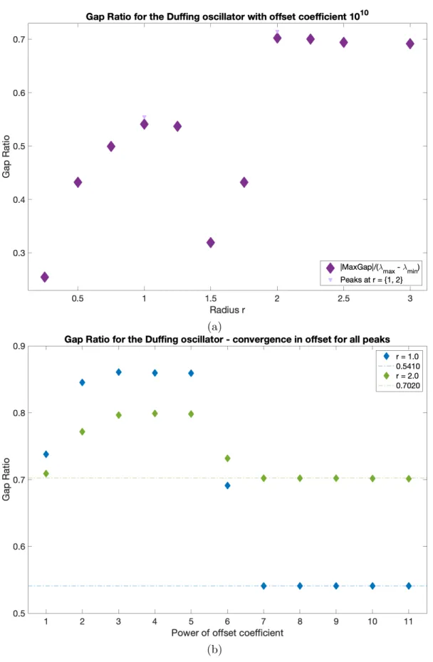
coherence metrics under noise. . . 80 2-17 The Duffing oscillator. (a) Poincar´e map with 1000 periods of perturbation

Tpert = 2π/ω. (b) Forward time FTLE for 30Tpert, time chosen for the spectral

clustering analysis. (c) FTLE ridges in forward (red) and backward (green) time for 10Tpert. (d) Superimposed forward (positive, red tones) and backward

2-18 Steps 1 and 2 of the spectral clustering protocol for the Duffing oscillator. . . 83

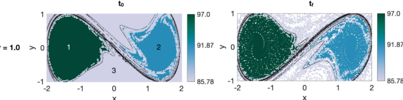
2-19 Step 3 of the spectral clustering protocol for the Duffing oscillator: results with coherence metrics under noise. The FTLE ridges are superimposed and correspond to the boundaries of the clusters. . . 84

2-20 Boundary calculations for the single connected set within the Duffing oscilla-tor, detected withr = 2.0. . . 84

2-21 The asymmetric Duffing oscillator. (a) Poincar´e map with 1000 periods of perturbation Tpert. (b) Forward and (c) backward FTLE for 10Tpert. . . 86

2-22 Steps 1 and 2 of the spectral clustering protocol for the asymmetric Duffing oscillator. . . 88

2-23 Step 3 of the spectral clustering protocol for the asymmetric Duffing oscillator: results with coherence metrics under noise perturbation. The FTLE ridges are superimposed and correspond to the boundaries of the clusters. . . 89

2-24 Coherence metrics applied to closed orbits of the Poincar´e map of the asym-metric Duffing oscillator. . . 90

3-1 Connectivity matrix for the Hawaiian archipelago. Retrieved from NOAA Coral Reef Watch based on the works of Kolinski & Cox [2003]; Kool et al. [2010] . . . 93

3-2 Connectivity and LCS in Coral Bay, Australia. Figures and captions extracted from Leclair et al. . . 95

3-3 Location of the Scott Reef atoll system off the northwest coast of Western Australia (maps accessed in ESRI, ArcGIS). Figure and caption from Foster & Gilmour [2018]. . . 96

3-4 Bathymetry of Scott Reef from Raysonet al. [2018]. . . 97

3-5 Meshes used for the SUNTANS model runs. . . 100

3-7 (a) Spectral clustering and (b) FTLE analyses of the 2007 dataset for the

channel. Data from Alireza Hadjighasem. . . 102

3-8 Research Vessel Solander from the Australian Institute of Marine Science docked in Broome, Western Australia. . . 104

3-9 Surface drifters built ad hoc . . . 104

3-10 Release strategy for the drifters at Scott Reef . . . 106

3-11 Scott Reef field release: drifter trajectories. . . 107

3-12 Scott Reef field release Part 1. Comparison between the experimental drifter positions, the velocity field and the LCS analysis at the start of the release at (Left) 06:30 and (Right) 07:00. . . 110

3-13 Scott Reef field release Part 2. Comparison between the experimental drifter positions, the velocity field and the LCS analysis throughout the release at 07:30, time at which all drifters were in water; 10:00, roughly half-way through the 6-hour experiment; 12:00 at low tide and start of the flood; and 13:30, 6 hours after all drifters were in water. . . 111

3-14 FTLE fields in forward and backward times for Scott Reef South around (a) neap tide on September 27 and (b) spring tide on October 3. . . 113

3-15 FTLE fields in forward and backward times in the Scott Reef channel around (a) neap tide on September 27 and (b) spring tide on October 3. . . 115

3-16 Periodicity of the FTLE ridges around spring tide: superimposition of FTLE ridges (dark red) at 6 consecutive (a) highs and (b) lows of the tidal cycle. . 116

3-17 Step 1 of the spectral clustering protocol for the Scott Reef channel. . . 118

3-18 Step 2 of the spectral clustering protocol for the Scott Reef channel. . . 119

3-19 Step 3 of the spectral clustering protocol with coherence metrics for the Scott Reef channel. . . 120

3-20 Spectral clustering results for the Scott Reef high tide event with a 12-hour integration window, area shrinkage and vertical fluxes for the northern cluster over 12 hours. . . 121 3-21 Divergence in the Scott Reef channel before and after removing the divergent

component for (a) the neap tide event and (b) the spring tide event. . . 123 3-22 Forward FTLE fields in the Scott Reef channel for the non-divergent velocity

fields around (a) neap tide on September 27 and (b) spring tide on October 3. 124 3-23 Step 1 of the spectral clustering protocol for the non-divergent velocity fields:

high tide during (a) neap tide and (b) spring tide. . . 125 3-24 Step 3 of the spectral clustering protocol for the non-divergent velocity field

at high tide around neap tide: results with coherence metrics for the peak at

r= 0.025. . . 125

4-1 Google Earth satellite image of the region of interest around the island of Martha’s Vineyard, Massachusetts. . . 133 4-2 Bathymetry south of Martha’s Vineyard. Depths in meters. Data from MSEAS.135 4-3 CODE/DAVIS-type drifters. . . 138 4-4 LCS predictions for the August 14, 2017 No Man’s Land experiment. . . 140 4-5 CODE drifter trajectories for the August 14, 2017 No Man’s Land experiment. 143 4-6 (a) CODE drifter trajectories (thick blue lines) and numerical trajectories

individually seeded for each ensemble of the model (colored dotted lines). The release positions are shown in red crosses. (b) Pairwise distances between the experimental and numerical trajectories, for each ensemble and each drifter. (c) Same as (b) minus drifters 4-6. . . 145 4-7 LCS results for the August 14, 2017 No Man’s Land experiment. . . 147 4-8 LCS analysis for the August 14, 2017 No Man’s Land experiment: zoom in

on the clustering results. . . 151 4-9 LCS predictions for the August 7, 2018 No Man’s Land experiment. . . 155

4-10 CODE drifter trajectories for the August 7, 2018 No Man’s Land experiment from 16:00 to 22:00. . . 157

4-11 (a) CODE drifter trajectories (thick lines) and numerical trajectories (thin lines), individually seeded in TRACE from the MSEAS velocity fields. Each color correspond to a different drifter trajectory. (b) Pairwise distances be-tween the experimental and numerical trajectories for each drifter. The colors match those in (a). The average distance is plotted with the thick grey line. 158

4-12 (a) Wind data used by MSEAS forecasts. (b) Measured wind time series for August 7, 2018. . . 159 4-13 Tidal time series for August 7 and August 8, 2018. . . 161

4-14 CODE drifter trajectories (a) until August 15 12:00, 20 hours after the last drifter deployment and (b) from 04:00 to 10:00 on August 15. The drifter positions are color-coded by time. . . 162 4-15 (a) CODE drifter trajectories (thick lines) and numerical trajectories (thin

lines), individually seeded in TRACE from the MSEAS velocity fields, for 04:00 to 10:00 on August 15. (b) Pairwise distances between the experimental and numerical trajectories for each drifter. The average distance is plotted with the thick grey line. . . 163 4-16 LCS analysis for the August 8, 2018 No Man’s Land experiment. . . 167

4-17 Zoom on the coherent spectral cluster at 10:00 from figure 4-16. . . 168

A-1 Steps 1 and 2 of the spectral clustering protocol for the Bickley jet with the maximum distance function. . . 182

A-2 Step 3 of the spectral clustering protocol for the Bickley jet with the maximum distance function. . . 183

A-3 Steps 1 and 2 of the spectral clustering protocol for the Duffing oscillator. (Top) Sweep of r parameters with offset coefficient 1010 _{and the average}

dis-tance function. (Middle) Same for the maximum disdis-tance function. (Bottom) Sweep of offset coefficients 10n _{for the gap ratio peaks. . . 184}

A-4 Spectral clustering results for the Duffing oscillator with the maximum dis-tance function. . . 184

B-1 Comparison between backward-time FTLE ridge advected from 07:30 and computed backward-time FTLE fields on a sliding window covering the Scott Reef field experiment. . . 189 B-2 Comparison between backward-time FTLE ridge advected from 07:30 and

computed backward-time FTLE fields on a sliding window covering the Scott Reef field experiment (Part 2) . . . 190 B-3 Comparison between forward-time FTLE ridge advected from 07:30 and

com-puted FTLE fields on a sliding window covering the Scott Reef field experiment.191 B-4 Comparison between forward-time FTLE ridge advected from 07:30 and

com-puted FTLE fields on a sliding window covering the Scott Reef field experi-ment (Part 2). . . 192 B-5 Comparison between forward-time FTLE ridge advected from 07:30 and

com-puted FTLE fields on a sliding window covering the Scott Reef field experi-ment (Part 3). . . 193 B-6 Comparison between forward-time FTLE ridge advected from 07:30 and

com-puted FTLE fields on a sliding window covering the Scott Reef field experi-ment (Part 4). . . 194

C-1 Tidal time series for August 14, 2017. . . 198 C-2 Evolution of the FTLE field at different times of the tidal cycle for the day of

C-3 Sweep of r radii for the parameter-free spectral clustering protocol used for the analysis of the 2017 No Man’s Land experiment. (a) Sweep for the 14:20 to 20:20 time window. (b) Sweep for the 15:51 to 21:51 time window. . . 200 C-4 Sweep of offset coefficients for the r values corresponding to the peaks in gap

ratios from figure C-3. (a) Sweep for the 14:20 to 20:20 time window. (b) Sweep for the 15:51 to 21:51 time window. . . 201 C-5 Encounter volume over the entire domain of computations for the analysis of

the 2017 No Man’s Land experiment. (a) Results for the 14:20 to 20:20 time window. (b) Results for the 15:51 to 21:51 time window. (c) Results for the 21:51 to 03:51 time window. . . 203 C-6 Sweep of r radii for the parameter-free spectral clustering protocol used for

the analysis of the 2018 No Man’s Land experiment. Sweep for the 04:00 to 10:00 time window. . . 204 C-7 Sweep of offset coefficients for the r value corresponding to the peak in gap

ratios from figure C-6. Sweep for the 04:00 to 10:00 time window. . . 204 C-8 Encounter volume over the entire domain of computations for the analysis of

the 2018 No Man’s Land experiment. (a) Results for the 04:00 to 10:00 time window. (b) Results for the 10:00 to 16:00 time window. . . 205

Chapter 1

Introduction

Ocean surface transport has been at the core of societal problems since the American Revo-lution: Benjamin Franklin, who charted the Gulf Stream as early as 1768, shared knowledge of its circulation patterns with America’s French allies, thereby giving them a maritime tac-tical advantage in the North Atlantic during the Revolutionary War. A 1786 version of this chart provided in figure 1-1 on page 22. Centuries later, transport in the ocean is still a topic of active research as many environmental disasters are related to ocean surface transport, including the spread of marine plastic pollution, the Deepwater Horizon oil spill and the nu-clear contamination from the Fukushima Daiichi plant. Understanding and predicting flow transport, however, remains a scientific challenge.

Building on the recent emergence of Lagrangian methods and other analytical tools from dynamical system theory, this thesis investigates the present-day abilities to describe and understand the organization of flow transport at the ocean surface, including the abilities to detect the underlying key structures, the regions of stirring and regions of coherence within the flow. The motivations for studying ocean transport and, particularly, surface transport are presented in section 2.1. Section 1.2 introduces the Lagrangian perspective to describing flow transport. Section 1.3 presents an introduction to Lagrangian Coherent Structures (LCS). Previous applications of LCS to oceanic flows are reviewed in section 1.4. Lastly, the

Figure 1-1: A chart of the Gulf Stream by Poupard & Franklin [1786]. Knowledge of the surface currents helped navigation of the North Atlantic.

overview of this thesis is presented in section 2.2.

1.1

The importance of ocean surface transport at the

submesoscale

As seawater flows throughout the global ocean, it advects its physical properties and tracers such as heat, nutrients and oxygen. The distribution of different water properties by ocean transport occurs throughout the water column: at the surface, in the deep ocean and at the intermediate upper ocean layer, the layer between the surface and the steep temperature gradient called the thermocline. The dynamics of ocean transport play a major role in regulating Earth’s climate [van Sebilleet al., 2018]. Ocean physics also impact marine ecology by shaping the environmental conditions around different ecosystems, including their access

to nutrients and light.

The ocean surface is of particular importance because it is the interface between the atmosphere and the ocean: air-sea interactions dictate processes such as heat transport [Thomaset al., 2008; Zhanget al., 2014], which are an essential component of climate models. Moreover, about 50% of oxygen on Earth results from photosynthesis by phytoplankton in the upper layer of the ocean [Field et al., 1998; Marinov et al., 2008; Mahadevan, 2016], typically located within the upper 100 meters. Satellites images of plankton blooms, such as the ones provided in figure 1-2 on page 24, exemplify the role of oceanic structures in transporting and confining nutrients and plankton [Sandulescu et al., 2007]: the chlorophyll marks the edges of the ocean eddies and vortices trapping the plankton.

Ocean surface transport is also at the core of several societal and environmental disasters [Poje et al., 2014]. As previously mentioned, knowledge of the Gulf Stream helped the American Revolution; a 1786 chart was provided in figure 1-1. In 2010, the Deepwater Horizon spill released four million barrels of oil into the Gulf of Mexico, according to an estimate from Crone & Tolstoy [2010], highlighting the importance of reliable forecasts of oceanic contaminant transport [Olascoaga & Haller, 2012]. Pictures of the spill are shown in figure 1-3 on page 25. The following year, an earthquake and a tsunami caused the Fukushima Daiichi nuclear power plant to discharge radioactive particles into the ocean: these tracers have then spread throughout the North Pacific Ocean [Rypina et al., 2013, 2014a], further showing the importance of understanding the pathways and barriers to transport in the ocean.

Ocean surface transport is a complex problem because it operates on multiple length- and time-scales that are set by the underlying dynamics. At large length scales, such as that of ocean basins, the ocean dynamics are mostly governed by the Earth’s rotation, by pressure and temperature gradients and by the small depth-to-length ratio, as the horizontal velocities are several orders of magnitude higher than the vertical velocities. At small lengthscales (∼ O(≤1m)), the flows are dominated by turbulence and are highly three-dimensional. In

Figure 1-2: Satellites images of plankton blooms trapped in eddies. (a) Phytoplankton blooms in the Drake Passage stretching about 1300 km and highlighting the multi-scale vortex structures. Image taken with the Visible Infrared Imaging Radiometer Suite on the Suomi NPP satellite (Credits: NASA/Norman Kuring). (b) Phytoplankton blooms (natural-color image) in the Baltic Sea captured by the Operational Land Imager on Landsat 8. (Credits: NASA/Joshua Stevens/U.S. Geological Survey.) (c) 150-km wide eddy off the South Africa coast captured by the Terra satellite with the Moderate Resolution Imaging Spectroradiometer (Credits: NASA/Jesse Allen). (d) Zoom in of the rectangular insert in

(a)

(b)

Figure 1-3: British Petroleum oil discarded into the Gulf of Mexico from the Deepwater Horizon spill. Photographic credits: (a) Beltr´a [2010] (b) Kari Goodnough/Bloomberg via Getty Images.

between lie the mesoscale and the submesoscale. Mesoscale motions are characterized by a small value of the Rossby number Ro = _LfU , where U and L are the characteristic velocity and length scales, respectively, f = 2Ω sin(φ) is the Coriolis frequency at latitudeφ and Ω is the angular frequency of planetary rotation. Small Romeans that the flow is in geostrophic balance constrained by the planetary rotation and the pressure gradient force: the Coriolis force dominates over the inertial and centrifugal forces. Typically, the mesoscale refers to scales ranging from 10 to 500 km [Abernathey & Haller, 2018].

At large lengthscales and mesoscales, oceanic flow processes have been extensively studied [Ferrari & Wunsch, 2009; Wunsch & Ferrari, 2018], but within the transition scale between the mesoscale and the small scale, dynamical features are less well understood [Thomaset al., 2008; Poje et al., 2014; McWilliams, 2016]. This transition scale is called the submesoscale: it is often defined dynamically by O(1) Rossby number Ro. Thomas et al. [2008] also characterize the submesoscale byO(1) Richardson number,Ri: Ri= _(du/dzN2 ₎2, wheredu/dzis

the vertical shear in velocityu(z) andN =

q

−g_ρdρ_dz is the Brunt–V¨ais¨al¨a buoyancy frequency, withg the local acceleration due to gravity andρ the density. For typical flow speeds of 0.10 ms−1_{,O(1) Rocorresponds to∼1 km in Massachusetts and ∼750 m at very high latitudes;}

Ro is undefined at the equator where f = 0. Typically, the submesoscale corresponds to lengthscales of O(1-10km).

Submesoscale processes are of particular interest for several reasons: just to name a few, they play a major role in the energy cascade towards smaller-scale dissipation, they are also relevant to primary productivity by phytoplankton [Mahadevan, 2016]. Understanding ocean surface transport at this scale is also of vital importance for the outcomes of search and rescue operations [Peacock & Haller, 2013; Allshouse & Peacock, 2015b], as drifts ofO(1-10km) are typically found to occur over 2–3 days. One major reason why dynamical features on the ocean surface are the least understood at the submesoscale is because they present what McWilliams [2016] calls “an observational barrier”: submesoscale processes have shorter spatiotemporal scales than mesoscale or larger features, making it hard to obtain a global

and continuous coverage of these processes with the required spatio-temporal resolution using standard technology and approaches [Zhang & Qiu]. For instance, present-day remote sensing offers global coverage of the Earth, but it only recently started offering the spatial accuracy required to observe submesoscale phenomena globally [McWilliams, 2016]; note that the temporal resolution required for a global coverage of submesoscale processes is still lacking. Smaller features, including fine-scale microstructures of ∼ O(≤1m)), can be measured with shipboard instruments [Seo et al., 2018; Shao et al., 2018; Sun et al., 2018]. Submesoscale processes, however, are too large and too rapidly evolving to be fully captured by typical ship surveys.

This thesis investigates the present-day abilities to describe and understand the organi-zation of flow transport at the ocean surface over the submesoscale range. It is primarily based on a series of field experiments that consisted of drifter releases. The LCS analysis is applied to numerical model data and compared to the experimental investigations, with the goal to evaluate our abilities to detect the underlying key structures, the regions of stirring and regions of coherence within the flow. This analysis is conducted through established LCS methods as well as an approach newly-developed as a part of this thesis, a parameter-free spectral clustering protocol with a noise-based metric to evaluate the coherence of clusters.

1.2

The Lagrangian versus Eulerian perspectives of

trans-port

The dynamics of motion in geophysical fluid flows and the patterns of transport can be described from the Eulerian perspective and the Lagrangian perspective. The Eulerian de-scription of fluids represents the flow motion as a function of position x and time t from a fixed reference frame, focusing on the properties of the flow within a domain at an in-stantaneous time: for example, through the velocity field v(x, t). Velocity is inherently a frame–dependent property and needs to be adapted to the frame of reference to describe the

Figure 1-4: A rotating saddle misclassified as a vortex by most nonobjective diagnostics. Figure and caption from Haller [2015].

material behavior. The Lagrangian description, in contrast, represents fluid motion by fol-lowing fluid parcels as they move through time and space and is a more natural perspective to study ocean transport [Davis, 1983; Mendoza & Mancho, 2012; Lehahn et al., 2018]. An-other important consideration to study flow transport is objectivity: the material response should be identified independently of the observer. A nice example that illustrates the need for objectivity is taken from Haller [2015] and provided in figure 1-4 on page 28: the closed and rotating streamlines around the red parcel of fluid can lead to the misclassification of this flow as elliptic or vortical. Advection of the red parcel, however, reveals that it is a ro-tating saddle flow. Had this parcel of fluid been trapped inside a coherent vortical structure instead, it would have stayed coherent over time.

For a given flow velocity field, the particle trajectories can be generated through the equation of motion:

dx

dt =v(x, t). (1.1)

The solutions are denoted byx(x0, t0;t), wherex0 is the initial position at initial timet0 and

t ∈ [t0;t1] is the time instant within the interval from the initial time t0 to the final time

t1. This relatively simple equation can nonetheless generate complicated trajectories, even

in time-periodic flows: indeed, the resulting trajectories can result in chaotic motion [Aref, 1984; Rypina, 2007]. Chaotic motion is defined by a high sensitivity to initial conditions, meaning that very small changes in initial conditions can result in vastly different trajectories: neighboring particles can separate exponentially with time. Aperiodic flows also commonly generate trajectories with such sensitive dependence on initial conditions [Haller & Poje,

1998]. Oceanic flows are aperiodic, even when they are driven by periodic forcing, such as tidally-driven flows in inlets or coral lagoons. Oceanic velocity fields are typically obtained from analytical models [McWilliams, 1976], numerical models [Deleersnijder & Lermusiaux, 2008; F.J. et al., 2013; Rayson et al., 2018], high-frequency radar systems [Rypina et al., 2014b; Kirincich, 2016], or satellite altimetry [Lehahn et al., 2018] .

The properties of distinct water parcels can be exchanged through homogenization via mixing, following the repeated stretching and folding of material surfaces, such as through mechanical swirling of the fluids. With stirring, the gradients between the water parcels increase sharply. Mixing is the second phase of homogenization and involves molecular diffusion. The processes governing stirring can be interpreted by the field of dynamical systems theory and its advances from the past 15–20 years [Haller & Yuan, 2000; Wiggins, 2005; Villermaux, 2019]. The patterns of transport can be recognized through the detection of areas with high rates versus low rates of stirring or through the detection of barriers to transport that can occur in a flow. Examples of the latter are plentiful in natural flows, including the smoke rings emerging from a puffing volcano, as shown in figure 1-5, oceanic and atmospheric fronts, the eddies shedding from the Gulf Stream or the vortices from figure 1-2. The Lagrangian structures that organize transport and govern coherent trajectory patterns over a given interval of time in such complex fluid flows are referred to as Lagrangian Coherent Structures (LCS), a term coined by Haller & Yuan [2000]. These structures act as the hidden skeleton of spatiotemporally complex fluid flows [Mathuret al., 2007; Peacock & Haller, 2013; Haller, 2015] and are often undetectable and unidentifiable from the direct interpretation of velocity fields in unsteady flows.

This thesis considers several tools used to identify LCS. The following section presents a brief overview of the LCS methods that will be discussed or used in this thesis. Two methods in particular will be further explained in chapter 2: the Fuzzy C-Means (FCM) and the spectral clustering methods, which aim to detect coherent parcels of fluid from clusters of particle trajectories. The other primary LCS tool used is the Finite-Time Lyapunov

Figure 1-5: Steam rings blown by Mount Etna in November 2013. Courtesy of Tom Pfeiffer

http://www.volcanodiscovery.com. Figure and caption from Haller [2015].

Exponent (FTLE), described in section 1.3.1, whose usability for planning experiments will be assessed in details.

1.3

Common LCS detection methods

LCS methods can be classified according to the type of structures they seek to detect. Some methods called cluster-based methods, such as Fuzzy C-Means (FCM) or spectral clustering, seek to detect parcels of fluids that remain coherent and non-filamenting over time, whereas other methods, such as the Finite-Time Lyapunov Exponent (FTLE) or the variational approach, look for the structures delimiting regions with qualitatively different transport be-haviors. Many LCS methods require large datasets of Lagrangian trajectories generated by velocity fields. This is the case for the FTLE, the most widely used method that is described in subsection 1.3.1, which requires a greater resolution than, for instance, cluster-based meth-ods. In contrast, some methods, like braid theory, have been developed to specifically analyze sparse datasets of trajectories, as dense datasets of Lagrangian trajectories are sometimes difficult to obtain.

Recent review papers of LCS methods include Allshouse & Peacock [2015b] and Had-jighasem et al. [2017]. Two cluster-based methods, FCM and spectral clustering, briefly summarized in subsection 1.3.2, will be further discussed in chapter 2. The encounter

vol-ume method, explained in subsection 1.3.3, will also be used in chapter 4. In chapters 3 and 4 of this thesis, the analysis of the case studies was based on numerical ocean models.

1.3.1

Finite-Time Lyapunov Exponent

In 2000, Haller & Yuan coined the term of Lagrangian Coherent Structures (LCS) and defined these structures as the “material lines with locally the longest or shortest stability or instability time”. They computed fields of Finite-Time Lyapunov Exponents, or FTLE, from particle trajectories to look at LCS boundaries. Since then, the FTLE approach has remained the most widely used LCS method. FTLE fields can be computed by the differentiation of the flow map, obtained from numerical trajectories xj(x0, t0;t), typically generated from

velocity field datasets with high resolution, over a finite integration time t ∈ [t0;t1] from

initial conditionsx0. The flow map at time t is denoted by Ftt0 :=xj(t0, x0;t). The gradient

of the flow map is used to compute the Cauchy-Green strain tensor:

C_t0t1(x0) = ∇Ft1_t0(x0) T ∇Ft1_t0(x0) (1.2)

as well as its eigenvalues λi(x0). For a forward-time flow map, the largest eigenvalue yields

the largest amount of stretching possible between neighboring tracer particles. It is used to construct the scalar FTLE field and quantify the separation rate within the flow over [t0;t1].

Λt1_t0(x0) =

1

t1−t0

logpλn(x0). (1.3)

Here, Λt1_t0(x0) is the FTLE value at the position x0 for the integration window [t0;t1], n is

the number of dimensions of the trajectories, withn = 2 for a two-dimensional flow, andλn

is the highest eigenvalue.

Locally maximum values of FTLE that are connected along a curve, referred to as FTLE ridges [Shadden et al., 2005], correspond to structures with the strongest separation rates for forward time advection: the separation of particles for the time window considered is

maximal on each side of the structures. These structures are thus often called ‘repelling’ [Hadjighasem et al., 2017]. Conversely, FTLE ridges of backward-time calculations from t1

to t0 are the curves along which the strongest attraction rates occur in forward time and

they identify locally attracting features.

For any LCS method, the analysis of a dynamical system depends on the time window of integration from t0 to t1: this time window is a property of the system that is analyzed

rather than a parameter of the method. It also depends on the resolution of the numerical grid, i.e., the number of particles included for the computations: it must be sufficient for the method of interest, which can be verified by the convergence of results when the resolution is increased. The FTLE analysis depends on the time window and the numerical grid, but no parameters are needed, making this method very advantageous. It is important to note that the FTLE fields and/or ridges are computed for the chosen window of time t0 tot1. FTLE

fields are often computed sequentially over sliding integration windows [t0+dt;t1+dt] to look

at how the organization of a flow evolves in time. The corresponding FTLE ridges are not time-evolving structures, as they are sequentially recomputed: indeed, each [t0+dt;t1+dt]

interval represents a different finite-time dynamical system. The sliding-window analysis is however commonly performed [Shadden et al., 2005; Hadjighasem et al., 2017], but it is important to note that the sliding window analysis looks at the LCS within a dynamical system evolving from t0 to tf as opposed to the evolving LCS of the dynamical system at

time t0. An example of the differences between advected FTLE ridges and sliding-window

FTLE computations is provided for the case study in chapter 3, in appendix A-2.

1.3.2

Cluster-based methods

Cluster-based LCS methods detect groups of particles that form coherent sets isolated from the rest of the flow. Recently, methods have been developed based on algorithms from unsupervised machine learning, in which all individual particles are assigned to a cluster in an automatic way. The two cluster-based methods, Fuzzy C-Means and spectral clustering,

will be detailed and discussed further in chapter 2 and applied throughout this thesis. The Fuzzy C-Means (FCM) approach to LCS detection introduced by Froyland & Padberg-Gehle [2015] is a clustering algorithm that assigns particles to clusters based on the Euclidean distance between trajectories. The FCM algorithm allocates the trajectories according to the average over time of the geometrical distance between trajectories and cluster centers. The partition of the domain is optimized when the trajectories are close to their assigned clus-ter’s center. This optimization is iterated through the particles’ likelihoods of membership to different clusters.

The spectral clustering approach [Hadjighasem et al., 2016] also detects coherent clus-ters based on the distance between trajectories, but with weights that quantify pairwise similarities between trajectories, using tools from spectral graph theory. Spectral clustering assigns particles to different clusters in order to maximize the intra-cluster similarity while minimizing the inter-cluster similarity. Domains filling the space between coherent clusters correspond to the incoherent cluster, or mixing regions.

1.3.3

Non-exhaustive review of LCS methods

One of the first methods developed to detect coherent sets from sparse trajectories was the braid theory approach by Thiffeault [2010]; Allshouse & Thiffeault [2012]. It transposes the time-evolving trajectories into a two-dimensional space-time diagram, which highlights how trajectories intertwine, thereby reducing the data to a sequence of crossings between trajectories. The method measures the rate of topological entanglement of these trajectories and defines coherent groups from sets of particles with minimal entanglement compared to the rest of the dataset. To analyze a set of trajectories over a certain time interval T, the only parameter to pick is the ratio of entanglement, which distinguishes the coherent sets from the rest of the system where entanglement, and thus mixing, is much higher. However, to yield any result, braid theory necessitates the coherent sets to contain at least a couple of particles with a rate of entanglement much lower than the surrounding region of mixing. The

main drawback of applying the braid theory approach to geophysical flows is that the method requires a certain amount of entanglement of trajectories, as well as a range of entanglement levels that is wide enough to detect coherent group: in open domains, such as oceanic flows, the required coverage of trajectories in space and time is nearly impossible to obtain in field experiments.

The complexity method (CM) was developed by Rypina et al.[2011] to sort trajectories within a domain according to their levels of complexities. The method measures the cor-relation dimension of trajectories and their ergodicity defect d. The correlation dimension

c∈ [0,2], where c = 0 corresponds to stationary points, c = 1 to smooth curves and c = 2 to chaotic curves densely covering an area, allows to distinguish relatively complex trajec-tories from less complex trajectrajec-tories. duses a counting method similar to box counting and measures the deviation from ergodic motion. The trajectory complexity method requires a parameter beyond the grid resolution and the time window of integration: the number of sampled points along the trajectories. It also requires that the boxes in the box counting method decrease from the full domain to a domain small enough.

Rypina & Pratt [2017] also developed the encounter volume method, which computes the volume of fluid that a given trajectory encounters over a finite interval. The encounter volume gives an indication of the mixing potential of the flow: a low encounter volume characterizes, for example, the cores of coherent eddies; a high encounter volume characterizes chaotic regions. The encounter volume is calculated from the number of trajectories passing by a reference trajectory within a threshold distance, the encounter radius, over a time interval

T; this threshold is the only parameter to be picked by the user for the encounter volume method, along with the numerical grid resolution and the window T. Another advantage of the encounter volume is that, similarly to the FTLE, it is a visualization of the kinematics of the flow that displays both the regions of low mixing and of high mixing. It reveals where water parcels can exchange water properties and gives an estimate for the mixing potential of the flow. The encounter volume can also be connected to diffusivity [Rypinaet al., 2018].

Serra & Haller [2016] also looked at the differentiation of the flow map, but using the rate-of-strain tensor and the initial-time Taylor expansion of the Cauchy-Green strain ten-sor. In the limit of a small integration window, the Eulerian rate-of-strain tensor governs Lagrangian deformation. The Eulerian Objective Coherent Structures (OECS) are defined as the instantaneous limits of Lagrangian coherent structures. One advantage of OECS is that the computations rely on the velocity field and do not require the generation of trajec-tories. OECS are frame invariant, but they are not Lagrangian. The only parameter needed is the numerical grid resolution.

The geodesic approach by Haller [2015] applies principles from variational calculus to ma-terial surfaces to find extremizing functions. Repelling shrink– or strain–lines and attracting stretchlines are detected from the first and second eigenvectors of the Cauchy-Green strain tensor, respectively, which constitute hyperbolic LCS [Farazmand & Haller, 2012]. Alter-nating chains of strainlines and stretchlines connecting singularities of the Cauchy-Green tensor form parabolic LCS that minimize Lagrangian shear and are jet cores [Farazmand

et al., 2014]. Elliptic LCS are detected through the computation of material-line-averaged stretching; closed material lines for which the stretching is of the same order as neighboring material curves are the elliptic LCS. The outermost closed shear line marks the boundaries of coherent vortices [Haller & Beron-Vera, 2013]. A drawback of the geodesics method is the number of parameters it requires, including, among others, the distance threshold between singularities for computing parabolic LCS.

Rotationally coherent LCS are defined by Farazmand & Haller [2016] as material sur-faces whose elements experience identical rotation over a finite time interval. The polar rotation angle (PRA) is computed from the flow gradient ∇F_t0t1(x0) to detect the

bound-aries of rotationally coherent vortices from the outermost closed and convex level curves of the PRA. Building on the rotation angles theory, Farazmandet al. [2016] propose to use the Lagrangian-Averaged Vorticity Deviation (LAVD), which is the trajectory-averaged, normed deviation of the vorticityω(x(t;x0)) from its spatial mean ¯ω, to identify rotationally coherent

LCS. The choice of the outermost convex contour is somewhat arbitrary.

Similarly to the FTLE, the Finite-Size or Finite-Scale Lyapunov Exponent (FSLE) method [Artale et al., 1997; Aurell et al., 1997] looks at separation in the flow by computing how fast the distance between neighboring trajectories reaches a certain threshold value. The FSLE approach, however, is not as widely used as other LCS methods such as the FTLE: it performs better at larger spatial scales [LaCasce, 2008] and it does not distinguish the different spatial scales of a system. Ultimately, it is unreliably sensitive to the temporal resolution of velocity fields at small scales [Hadjighasem et al., 2017].

1.3.4

Bickley Jet example

Most methods mentioned in sections 1.3.1–1.3.3 are illustrated in figures 1-6–1-7 on pages 37–37. The example is the Bickley Jet flow, which will be further detailed in the following chapter. It consists of a zonal jet that is a barrier to meridional transport with three recircu-lation vortices on each side. The Bickley Jet is a benchmark flow in dynamical system theory because it exhibits transport behaviors that are qualitatively different and are common in realistic ocean flows: the jet, the vortices and the background chaotic zone.

In figure 1-6, panel (a) shows the Poincar´e section, which was computed here for the periodic Bickley jet with the parameters as in Rypina et al. [2007]. The Poincar´e section is a long-established methodology in dynamical system theory to study periodic flows: this stroboscopic mapping plots the trajectory positions at each period. Figure 1-6.(a) reveals how the jet acts as barrier to transport, as well as the presence of vortices corresponding to concentric discretely-sampled closed orbits, which are islands of coherence among the incoherent background. In contrast, the stroboscopic mapping of the particle trajectories outside these closed orbits show clouds of dots corresponding to the chaotic regime of the incoherent background. The six vortices are all of similar sizes.

Panels (b)-(i) in figure 1-6 were taken from Hadjighasemet al.[2017], in which the Bickley Jet was modified from Rypina et al. [2007] to become quasi-periodic. Because the flow is

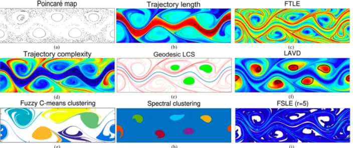
Figure 1-6: Comparison of Lagrangian methods on the Bickley jet example (forward-time calculations only). (a) Poincar´e section computed for the parameters in Rypina et al.[2007] corresponding to the periodic Bickley Jet flow. (b)-(j) Results of LCS methods on the quasiperiodic Bickley jet example. The panels were adapted from Hadjighasemet al.[2017].

Figure 1-7: Encounter volume for the periodic Bickley jet flow using encounter radius 5×105. Figure adapted from Rypina & Pratt [2017]

not periodic, the Poincar´e section could not be constructed, but the quasi-periodic system is qualitatively similar to the periodic system. The methods that will be used for analysis in chapters 2–4 of this thesis are the FTLE (figure 1-6.c), FCM (figure 1-6.g), spectral clustering (figure 1-6.h), FCM (figure 1-6.g) and encounter volume (figure 1-7). The flow used to calculate the Poincar´e section in figure 1-6.a corresponds to the flow used for the encounter volume method in figure 1-7, the periodic Bickley Jet. The trajectory complexity (figure 1-6.d), the geodesics approach (figure 1-6.e), the LAVD (figure 1-6.f) and the FSLE (figure 1-6.i) are included for completeness and because they are compared with the other methods throughout this thesis, including in section 1.4 and in chapter 2.

Figure 1-6.(b) shows the trajectory length, which corresponds to an arc length computa-tion of the distance covered by the adveccomputa-tion particles, as introduced by Manchoet al.[2013]. It is not an LCS method per se: just as trajectory complexity, FSLE or even FTLE, it does not define what the sought coherent structure are, but it provides an illustration of transport within the domain of interest. Figure 1-6.(b) shows the contrast between the meandering jet, with high values of length in red, and the cores of the recirculation vortices, in light blue. The vortices are hard to discern, however, as there are no clear vortex boundaries.

For the Bickley Jet, various methods captured different aspects of transport within the flow. In the Poincar´e section (figure 1-6.a), the closed orbits and the islands of coherence they bound were of similar sizes, suggesting that the vortices detected by LCS method should also be of comparable size. The FTLE scalar field (figure 1-6.c) reveals useful information about the differences in separation rates within the flow, but the individual vortices are hard to discern. The core of the jet shows minimal rates of separation, in blue, consistent with the notion of transport barrier, whereas the boundaries of the jet show maximal rates of separation, in red. The vortices are hardly delimited, however, as the FTLE values smoothly go from blue to green away from the core. While the shape of the jet can be discerned, the vortices are hard to bound. The trajectory complexity (figure 1-6.d) most clearly highlights the meandering jet through its very low values, in dark blue; the vortices are discernible

through relatively low values shown in blue, but the exact boundaries are hard to extract. The geodesic approach (figure 1-6.e) successfully detects the core of the meandering jet as a parabolic LCS, in blue, but only identifies three out of six vortices, the elliptic LCS, in green. The LAVD (figure 1-6.f) method successfully extracts the boundaries of the cores of the vortices, although the cores vary in areas. The jet is also characterized by low values, in blue, but its boundaries are not extractable. The FCM method (figure 1-6.g) can roughly detect the vortices as different clusters, but one vortex is missing its core and the method also includes very distant filaments in the clusters, which contradicts the definition of a coherent structure. These filaments indicate that the coherent sets include trajectories much further than the core of the clusters. The shape and size of the clusters vary highly, in contradiction to the orbits shown in the Poincar´e section, which are of similar size. Spectral clustering (figure 1-6.h) successfully detects each of the cores of the recirculation vortices as individual clusters. Moreover, these vortex cores are of similar sizes. The FSLE field (figure 1-6.i) shows the vortices as having low values, but the discrepancy in shape and size of the low FSLE regions make it nearly impossible to extract the coherent structures present in the flow. The jet is hardly discernible. Lastly, the encounter volume method (figure 1-7) also outputs a field that is a representative depiction of the flow transport: the cores of the recirculation vortices have very low encounter volume, in dark blue, consistent with the low mixing potential inside a coherent vortex. The jet core displays a low encounter volume and is delimited by the regions exhibiting high encounter volumes, in red, which is also consistent with high mixing potential.

To summarize, the output of LCS methods generally provides a picture of flow transport within the domain of interest and explains how transport is organized in the flow by revealing its key structures. Different LCS methods emphasize different properties of the flow; for this reason, it is expected that they capture different types of structures. No method is able to detect all the features of interest: here in figure 1-6, no method was able to rigorously extract the jet and the 6 recirculation vortices. Lastly, most methods depend on several user-input

parameters. In chapter 2, this thesis develops an improved parameter-free spectral clustering method. The applicability of different LCS methods, including the chapter 2 parameter-free spectral clustering, to geophysical flows will be assessed in chapters 3 and 4.

1.4

Previous applications of LCS to ocean surface flows

LCS are ubiquitous in the ocean: fronts that generate filaments often correspond to hyper-bolic structures; elliptic LCS are Lagrangian vortices or eddies; parahyper-bolic LCS are shearless cores of jets [Haller, 2015; Hadjighasem et al., 2017]. LCS have been computed in both measured and simulated realistic oceanic flows. They have been shown to underlie the orga-nization of transport of simulated tracers and real drifters.

There are multiple examples in which Lagrangian methods have been used to interpret the observed behavior of surface floaters, or drifters, including: Olascoaga et al. [2013]; Jacobs

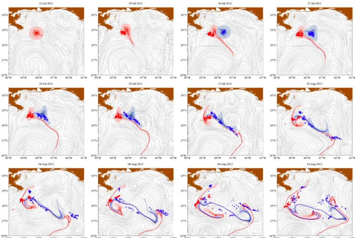
et al. [2014]; Beron-Vera et al. [2015]; Williams et al. [2015]; Rypina et al. [2014b, 2016]; Rypina & Pratt [2017].Typically, in these studies, high numbers of drifters were released and their trajectories were compared to the results from LCS analyses applied a posteriori to velocities from models, satellite altimetry or radar measurements. An example taken from Olascoaga et al. [2013] is provided in figure 1-8 on page 41, in which field drifter positions are compared to attracting LCS.

There are very few cases in which Lagrangian methods have actually been used to plan and execute field experiments. Hazaet al.[2007] and Hazaet al.[2010] computed FSLE fields from model forecasts for the DART experiment in the Adriatic sea, predicting high relative drifter dispersion. The model was enhanced with high frequency (HF) radar data collected during the drifter experiments. They released surface drifters for a series of consecutive days, with one- or two-day intervals, using the FSLE predictions as a guide. In both studies, the observed trajectories followed a behavior similar to those predicted from the model FSLE fields, as shown in figure 1-9 on page 43. The FSLE, as mentioned in the previous section,

Figure 1-8: Sequence of selected snapshots of the evolution of fluid patches as advected by the altimetry-derived velocity field (4) (red and blue areas) and corresponding centerpieces or attracting LCS obtained as the advected images of forward stretchlines through the patches at the initial time (red and blue curves). Also indicated are S1 (red dots), S2 (blue dots) drifter positions, and instantaneous streamlines of the altimetry-derived velocity field (gray curves). Figure and caption from Olascoaga et al. [2013].

is however not widely used for LCS detection anymore as it blends the input timescales [LaCasce, 2008].

To the knowledge of the author, no other field studies have used the by-now standard FTLE method, or other recently-developed set-based methods, to plan and support targeted drifter deployments in regions of distinct transport behavior. The field studies described in the following chapters therefore present the first experiments targeting FTLE ridges and coherent clusters of trajectories, investigating the utility of such Lagrangian methods for operational planning and execution.

1.5

Thesis overview

With the recent emergence of a multitude of LCS methods [Allshouse & Peacock, 2015b; Hadjighasem et al., 2017], the primary objective of this thesis is to advance the theory of LCS and then to evaluate the robustness and field applicability of a few common approaches, with a focus on our ability to predict LCS in submesoscale ocean surface flows, given all the uncertainties of the modeled and observed velocity fields, as well as the limitations of the LCS identification methods and the sparsity of Lagrangian data. This includes the design and execution of field experiments targeting LCS from predictive models and their subsequent Lagrangian analysis.

This thesis is organized as follows. A background on LCS and their applications to oceanic flows was given in sections 1.3–1.4. Chapter 2 introduces a new, parameter-free protocol for spectral clustering and proposes a metric for evaluating the coherence of the resulting clusters. The two subsequent chapters are organized around case studies: chapter 3 focuses on a field experiment carried out at Scott Reef, an atoll system in Western Australia, in October 2016, and chapter 4 details two field experiments carried out offshore Martha’s Vineyard, Massachusetts, in August of 2017 and of 2018. For all case studies, the velocity data from numerical models, either forecasting or nowcasting, was provided by collaborators,

Figure 1-9: (Left panel) Spatial distribution of FSLEs (in per day) computed forward in time (positive) and backward in time (negative) with the observed drifters in cluster 1. (Right panel) The main FSLE ridges that appear to be controlling the drifter trajectories. Figure and caption from Hazaet al. [2010].

as explained in the respective chapters and in the acknowledgment section. I processed and analyzed the resulting data in the framework of LCS to output predictions of key attracting or repelling LCS structures, as well as the most coherent regions. I planned and executed the bulk of the drifter releases around the predicted structures. In chapters 3 and 3, I will evaluate the comparison between the trajectories and the LCS predictions. Causes for the disagreement will be studied. The methods, models, instrument development and technology used in each case will also be discussed.

Chapter 2

A parameter-free spectral clustering

approach with noise-based cluster

coherence metrics

Recent advances in machine learning have led to an increased popularity of the field, which has been utilized in a very broad range of applications, with other disciplines progressively adopting machine learning methods. The field of Lagrangian Coherent Structures (LCS) has embraced several cluster-based algorithms and adapted the methods to LCS detection. These unsupervised machine learning approaches having emerged so recently, the robustness and applicability of these tools is yet to be proven, especially for geophysical flows. A recurring concern is that the clustering results tend to be highly sensitive to the parameter choices. Building upon the method developed by Hadjighasem et al. [2016], an updated spectral clustering approach is presented that avoids arbitrary parameter choice.

The merits and limitations of clustering methods for LCS detection are argued in section 2.1. An overview of commonly used methods is given in section 2.2. Section 2.3 presents the proposed updates to the spectral clustering approach and the noise perturbation metrics to quantify coherence within the clusters. The approach is applied in section 2.4 to three

idealized model flows: the Bickley Jet, the Duffing oscillator and the asymmetric Duffing oscillator. Concluding remarks are presented in section 2.5.

2.1

Motivations

A review of commonly-used Lagrangian approaches was given in chapter 1, which presented how LCS methods can be classified into those looking for coherent parcels of fluid and those looking for the structures delimiting regions of different transport behaviors. In their comparison paper, Hadjighasem et al. [2017], hereinafter referred to as HA17, classify LCS methods into two groups: diagnostic methods and analytical methods. From the properties of the input dataset of trajectories, diagnostic methods output scalar fields that emphasize the different features of flow transport; analytical methods, on the other hand, use rigorous mathematical principles to define coherence and detect LCS as the solutions of the formu-lated problems. Analytical methods perform well at detecting the barriers to transport in complex fluid flows: they include the geodesics approach, which has been used for example to detect finite-time mixing barriers in Jupiter’s atmosphere [Hadjighasem & Haller, 2016]; and the Lagrangian-averaged vorticity deviation (LAVD), which has enabled the extraction of eddies in a simulation of the Gulf of Mexico [Beron-Vera et al., 2018]. HA17 include cluster-based methods as analytical methods: these methods assign trajectories to different coherent groups. The clustering algorithms rely on heuristic arguments, however, and so it is considered in this thesis that cluster-based methods are somewhat different from analytical methods, but nevertheless reveal valuable information about the system of interest.

Analytical methods such as the geodesics approach, LAVD or the Polar Rotation Angle (PRA) perform very well for vortices with minimal leakage. Examples of the two methods are provided in figure 2-1 on page 48. The LAVD method in particular was developed to detect the boundaries of Rotationally Coherent Lagrangian Vortices (RCLV). Indeed, the vortex boundaries determined by PRA or LAVD display tangential filamentation only. For

other, non-vortical coherent structures, however, these methods would not necessarily be able to detect structures that stay coherent over [t0;t1] while having their shape deformed

or exhibiting some filamentation. LCS that may not exhibit the same behavior as a leakage-free vortex can still be of interest for the study of flow transport and are ubiquitous in the ocean. It is therefore argued in this thesis that cluster-based methods are relevant and useful for the detection and analysis of LCS in geophysical flows, being complementary to more mathematically rigorous methods.

Cluster-based LCS methods, such as Fuzzy C-Means, K-Means or spectral clustering, which are all borrowed from unsupervised machine learning, can provide information about non-vortical yet coherent regions by partitioning the domain into several clusters. A draw-back from many machine learning techniques is that the results rely on a set of user-input parameters. The choice of these parameters is often subjective and influenced by the user’s biases, which often affects the resulting analysis. HA17 describe how to “choose a reasonable set of parameters for each method” in order to yield “the most favorable outcome”. They describe a robust outcome as an outcome where “small variations in the parameters do not lead to drastic changes in the outcome”, which is a fair way to describe robustness. The reasonability of the parameters and the favorability of the outcome, however, suggest that, in the end, the user will have to make decisions about the outcomes of the analyses that could be arbitrary and subjective. Building on their efforts, this thesis addresses the need for a new protocol to carry on the spectral clustering analysis that, firstly, needs as few user-input parameters as possible and that, secondly, yields unbiased results, in the sense that the protocol should yield optimal results without any need for the user to decide between different outcomes. Optimal results, here, are defined by measuring the coherence of the clusters as robustness under noise; an optimal cluster partition is one where the clusters are the most coherent in comparison to the incoherent background. This metrics for coherence addresses another shortcoming of cluster-based method: once vortices or other isolated is-lands of coherence occurring in the flow are detected by any of the LCS methods, there is