Preprint typeset using LATEX style AASTeX6 v. 1.0
MOSFiT: MODULAR OPEN-SOURCE FITTER FOR TRANSIENTS
James Guillochon1, Matt Nicholl1, V. Ashley Villar1, Brenna Mockler2, Gautham Narayan3, Kaisey S. Mandel4,5, Edo Berger1, Peter K. G. Williams1
1Harvard-Smithsonian Center for Astrophysics, 60 Garden St., Cambridge, MA 02138, USA 2Department of Astronomy and Astrophysics, University of California, Santa Cruz, CA 95064, USA
3Space Telescope Science Institute, 3700 San Martin Drive, Baltimore, MD 21218, USA 4Institute of Astronomy and Kavli Institute for Cosmology, Madingley Road, Cambridge, CB3 0HA, UK 5Statistical Laboratory, DPMMS, University of Cambridge, Wilberforce Road, Cambridge, CB3 0WB, UK
ABSTRACT
Much of the progress made in time-domain astronomy is accomplished by relating observational multi-wavelength time series data to models derived from our understanding of physical laws. This goal is typically accomplished by dividing the task in two: collecting data (observing), and constructing models to represent that data (theorizing). Owing to the natural tendency for specialization, a disconnect can develop between the best available theories and the best available data, potentially delaying advances in our understanding new classes of transients. We introduceMOSFiT: the Modular Open-Source Fitter for Transients, a Python-based package that downloads transient datasets from open online catalogs (e.g., the Open Supernova Catalog), generates Monte Carlo ensembles of semi-analytical light curve fits to those datasets and their associated Bayesian parameter posteriors, and optionally delivers the fitting results back to those same catalogs to make them available to the rest of the community. MOSFiT is designed to help bridge the gap between observations and theory in time-domain astronomy; in addition to making the application of existing models and creation of new models as simple as possible,MOSFiTyields statistically robust predictions for transient characteristics, with a standard output format that includes all the setup information necessary to reproduce a given result. As large-scale surveys such as LSST discover entirely new classes of transients, tools such as
MOSFiTwill be critical for enabling rapid comparison of models against data in statistically consistent, reproducible, and scientifically beneficial ways.
Keywords: supernovae: general — methods: data analysis — methods: numerical — methods: sta-tistical — catalogs
1. INTRODUCTION
The study of astrophysical transients provides a unique opportunity to explore the interplay of physical laws for states of matter that are not easily reproducible in Earth-based laboratories. While the modeling of steady-state systems can yield valuable information on physics un-der fixed conditions, the dominance of different physical processes at different times in a given transient’s evo-lution means that tight constraints can be placed on these processes by self-consistent modeling of their time-dependent, observable features.
Transient characterization extends thousands of years to the first supernovae observed in antiquity, and the dataset has grown to be very rich in the past century at the same time that astronomical methods have become more rigorous. Over the past several decades, technol-ogy for collecting time-domain data has changed from predominantly photographic plates to charge-coupled
de-jguillochon@cfa.harvard.edu
vices, and the standards for characterizing the brightness and color of transients has evolved in tandem. Some of the best-characterized transients date from an era be-fore cheap computation and storage became ubiquitous, and are often not published with enough corresponding information to enable robust reproduction of observed data by models (information such as bandset, instru-ment, and/or magnitude system employed for a given observation). This means that the first step to modeling a given transient may involve contacting several people involved in the original study, a process which greatly slows the rate of scientific exploration.
The complete collection of observed transient data by astronomers has grown to a level that is easily charac-terizable as “big data,” a feature that will become more pronounced in the era of large-scale all-sky surveys that will (in the case of LSST) yield∼20 TB of imaging data every day (Abell et al. 2009). The products that are of interest for transient modeling (primarily photometry
and spectra) is however very manageable, with the to-tal dataset presently being.10 GB in size (Guillochon et al. 2017), small enough to fit comfortably on a mod-ern smart phone. But while the total number of known transients is expected to grow significantly in the com-ing decade, the identity of many transients will likely be difficult to determine given the limited spectroscopic follow-up available to the community. This lack of iden-tification and characterization can reduce the utility of future surveys which have the potential to increase tran-sient populations by orders of magnitude.
Open catalogs for astronomy (Rein 2012; Guillochon et al. 2017; Auchettl et al. 2017) aim to address these issues by agglomerating and crowd-sourcing data asso-ciated with each transient from the original publica-tions, private communicapublica-tions, and publicly available re-sources. Such catalogs enable observers to easily compare their data to previously published works, identify tran-sients that are similar to trantran-sients in their own datasets, and combine their own data on individual events with that from other researchers.
But while the availability of time-domain data has im-proved significantly, publicly accessible models of tran-sients have remained elusive (we are aware of one other service that offers conditional public access to supernova models, SNAP, Bayless et al. 2017). Individual works have focused on small subsets of data, offering descrip-tions of either light curve shapes or distribudescrip-tions of phys-ical parameters for a given set of transients, but the spe-cific data products depend heavily on the scientific moti-vations of the study in question. At present, reproducing a given model often requires a complete rewrite of the expressions presented by the original authors who put forward the model, which means that successful models are often times those that are simplest for others to im-plement, as opposed to models that best reproduce the observations.
Even in the cases where data are readily available, in-completeness in how the data are presented or ingested into catalogs can lead to the propagation of errors: for example, no distinctions between upper limits and de-tections, or misreporting of the magnitude system used (AB or Vega). In such cases, applying a well understood model, ideally calibrated against similar transients in the literature, can help to flag up potential errors through unrealistic model parameters or unexpectedly large resid-uals between model and data. Therefore if models are built to interact directly with transient catalogs, they al-low us to use our physical insight about the system to resolve issues of missing or incorrect metadata.
In this paper we present the Modular Open-Source Fitter for Transients (MOSFiT), a Python-based package released under the permissive MIT license that yields publicly accessible and reproducible models of transients.
This paper is intended to be a descriptive guide ofMOSFiT
and its capabilities upon its initial (version 1.0) release, but for an up-to-date user guide of the code the reader should consult the online documentation1. We note that
MOSFiT has already been used in the astronomical lit-erature in at least three studies (Nicholl et al. 2017b,a; Villar et al. 2017a).
In Section2we describe some of the concerns about re-producibility in astronomy, and lay out the guiding prin-ciples for the MOSFiT platform and how the code is de-signed to make time-domain science fully reproducible. Methods for inputting data intoMOSFiTare described in Section3, whereas the process for defining models in the code is described in Section4. Products of the code, and how users can share their results, are described in Sec-tion 5. Assessing model performance is covered in Sec-tion6, concluding with a discussion ofMOSFiT’s present-day shortcomings and future directions in Section 7.
2. END-TO-END REPRODUCIBILITY It is difficult to deny the massive impact the Inter-net has had upon science, especially open science efforts. Not only are scientific results immediately available via a wide range of media, but the full chain of software used to produce a scientific result is becoming increas-ingly available, even to the point where the platforms used to run a piece of scientific software can be repli-cated by third parties via virtual machines (Morris et al. 2017). This trend solidifies scientific results by ensuring that others can reproduce them (on a wide range of plat-forms via continuous integration services), enables third parties to identify possible problems in the software used to produce a given result, and fosters follow-up studies that may only require minor adjustments to an existent software stack.
These trends toward open access data policies have be-gun to take shape in the time-domain community, al-though much remains to be done. For time-domain as-tronomy, the issue of data access takes on a critical im-portance as every transient is a unique eventwhose data can only be collected oncethat will, at some level of detail, differ from every other transient previously observed, a situation that is far removed from laboratory-based ex-periments where identical conditions can be tested re-peatedly. Even if the transients themselves are almost identical, the observing conditions will almost certainly differ between transients.
For astronomy, a useful definition of a reproducible experiment is the series of steps (pipelines) required to convert raw observational inputs into scientifically-useful data products. These pipelines can in principle be re-run at a later date to ensure the data products were
MOSFiT
produced accurately, or to provide updated data prod-ucts if the methods contained within the pipeline have changed and/or more input data has become available in the interim. As publications do not yet provide reposi-tory hosting, the free hosting services offered by private companies such asgithubhas given viable options to ob-servers wishing to share their pipelines (for a recent ex-ample seeMiller et al. 2017). Describing a transient with a physical model can be viewed as one of the last steps in such a pipeline: once the observational data products have been produced, a piece of modeling software con-sumes those products and produces higher-level products of its own.
A complication is that the end-to-end pipeline, which ideally would extend from raw photon counts/images to physical parameter inferences, are distributed amongst a finite number of scientific groups that exchange the data to one another via scientific publications, private com-munications, or public data repositories, with no con-sensus on the best way to exchange such data (see Sec-tion5.1). Often times pieces of these pipelines are simply not available to the wider community, making a result reproducible only if all pieces of the pipeline are open and/or cooperative. This issue is particular acute on the modeling end of the pipeline, with off-the-shelf model-ing software only bemodel-ing available for the most commonly studied transients (e.g., SNooPy for Ia SNe,Burns et al. 2011).
While making source code for a project available is one of the first steps towards enabling others to reproduce your work (Baker 2016), true reproducibility across plat-forms is difficult to achieve in practice, especially for com-piled code where subtle differences in compiler behavior can yield different outcomes (Colonna 1996), particularly in chaotic systems (Rein & Tamayo 2017). While some projects have undertaken heroic efforts to ensure bit-for-bit consistency across a wide range of platforms ( Pax-ton et al. 2015), the required labor is often infeasible for smaller projects.
For optimization and sampling where stochastic meth-ods are employed, bit-for-bit reproducibility is less cru-cial, as random variations on the initial conditions should always converge to the same solution(s) anyway. Stochastic methods offer no guarantee however that they will converge in a finite time, particularly if they are prone to getting stuck in local minima, and the users of such methods should always be wary of this possibility. The determination of when an algorithm has converged to the solutions of highest likelihood can be bolstered by repeated runs of the stochastic algorithm and/or metrics for convergence that determine if the final distribution of likelihood realizations are well-mixed (see Section6).
2.1. Guiding principles and code design
Mindful of the issues mentioned above, the primary goal of MOSFiT is to make analysis of transient data re-producible and publicly available. The MOSFiTplatform has been written in Python, the most flexible choice at present for open source astronomy projects given the immense amount of development on astronomy-centric packages such as astropy, astroquery, emcee, and many others. Similar to the Open Supernova Catalog, we constructed MOSFiT with a set of principles to guide us when making various code design decisions. Our goals forMOSFiTas a platform are:
1. To enable the rapid construction and modifica-tion of semi-analytical models for transients such that scientists can react swiftly to newly-discovered transients and adjust their models accordingly (or to construct entirely new models).
2. To make the ingestion of historical and contempo-rary observational data as painless for the user as possible, and minimizing the need for scientists to scrape, annotate, and convert data into the proper input form.
3. To provide fits of models to data that are assessed by scoring metrics that are related to the total evi-dence in favor of a given model (as opposed to sim-ple goodness-of-fit tests), which have the potential to be used for model comparison.
4. To execute those models in a computationally effi-cient way that minimizes runtime and encourages users to optimize critical pieces of code that are likely shared by many models.
5. To provide predictions of the physical parameters responsible for an observed transient (e.g., ejecta mass or explosion energy) rather than shape pa-rameters that are not simply relatable to physical processes.
6. To distribute the work of modeling transients amongst scientists and the public and enabling sharing of their results to the broader community. 7. Finally, to enabling sharing of user fits to transients that are publicly accessible on a rapid timescale, potentially hours after a transient’s data is first made available.
More succinctly, MOSFiT should be easy, adapt-able, fast, accurate, transparent, andcommunity-driven. These goals are all served by making the platform open-source, well-documented, modular, optimized, and con-siderate of the astronomy software ecosystem both at the present day and in the future. MOSFiTis intended to be used by both observers and theorists, and so should
OSC and similar Model Description Posterior
+
Model Description Posterior+
Event B (JSON) Metadata Observations Derived parameters Model Description Posterior+
Event A (JSON) MOSFiT User #1 Model Description Posterior+
Event B (JSON) MOSFiT Model Repository Event A Event B MOSFiT User #2 Model Description Posterior+
Event B (JSON) Interested
parties
Bulk model
downloads Complete event downloads Web display
of models
Model from User #1
Model from User #2
Figure 1. Typical interactions of MOSFiT users with the Open Astronomy Catalogs and consumers of their data products. In the above example, twoMOSFiTusers (#1 and #2) submit model fits for two different events (A and B) to a model repository ongithubviaMOSFiT’s upload feature. The data in the model repository is then absorbed by the Open Astronomy Catalogs such as the OSC, which can then deliver event information to interested parties that contains observational data, model fits to that data, and any parameters derived from the model fits. The primary form of data exchange between various users and services areJSON files, displayed as light blue.
be useful to both parties; some should be able to use
MOSFiTas a development platform for constructing new transient models, whereas others should simply be able to useMOSFiTas a tool to match well-vetted models against new transients.
3. DATA INPUT
The story of how a particular photometric dataset makes its way from collection to publication differs on where the data was collected, who reduced the data, and how the data was presented. While any individ-ual dataset is usindivid-ually not too difficult to manipulate into a proper input format for a given code, the process can be extremely tedious if multiple datasets from multiple sources need to be converted. MOSFiT aims to simplify this process greatly by relying upon the Open Astronomy Catalogs2to provide sanitized, homogeneously formatted data, which can be optionally supplemented by the user’s own private data. The flow of data to and from the Open Astronomy Catalogs is shown in Figure1.
Our goal is to make the default choices of algorithms employed byMOSFiTrobust enough such that running a model fit against new data has the best possible chance of yielding an ensemble of model parameters that best explain the data. While there are always likely to be some transients where the data is not amenable to these default choices, the platform should be expected to more often than not return a meaningful result for a wide range of possible inputs.
2https://astrocats.space/
3.1. Using data from the Open Astronomy Catalogs Public data can be accessed directly by name from the command line using the data available in the Open As-tronomy Catalogs. As an example, the following com-mand will download all data for PS1-11ap and prompt the user to choose a model to fit against it:
mosfit -e PS1-11ap
For the user, this eliminates a significant amount of labor that might be involved in finding all the literature on this particular transient, collecting the fittable data from those sources, and combining the data into a com-mon format. It also means that independent users will have access to exactly the same data, which is not guar-anteed in cases where the original authors need to be contacted to acquire the data: the best available data from the original authors may change after publication as reductions are refined, either by the collection of bet-ter subtraction data or improvements in the reduction pipelines, meaning that supernova data is often not en-tirely stable.
3.2. Using private data and arbitrary input formats Ideally, part of the pipeline that processes data would yield data in a common schema that does not vary be-tween individual observers. A file’s format is one part of this schema, but a format alone is not enough, as for-mats do not specify key names or mandate which fields
MOSFiT
should be accompany a given type of data. The popular FITS standard3 is an example of a format widely used for its flexibility, with users appreciating the ability to specify whatever data structure best suits their partic-ular science need. But this flexibility comes at the cost of reproducibility, with the schema of individual FITS files often being poorly documented, making it difficult to decipher the data presented in a given FITS file.
Part of MOSFiT’s purpose is to assist the mission of converting the transient dataset, which is spread over tens of thousands of differently-formatted ASCII and bi-nary files, to a single schema, which is presently defined by the Open Astronomy Catalogs4. While many of the schema’s current properties have been decided in consul-tation with a small group of testers, the schema is not final and is intended to be modified in response to com-munity feedback.
As a large fraction of the available data is not in this format, aConverterclass (not itself a module as it is not required for model execution) is provided with MOSFiT
that will perform this conversion and feed the converted data into the Transient module. This class has been written to read ASCII data in a large number of com-mon formats: delimited tables, fixed-width CDS format, LaTeX tables, etc. As each table provided by a source is likely to use its own style of data presentation, the con-verter works through a series of logical steps to attempt to infer the table’s structure, and then prompts the user with a “choose your own adventure”-style questionnaire to determine structure details that it could not determine automatically. Once this conversion process is complete, the data is converted to Open Catalog format and fed into theTransientmodule.
As an example of the conversion process, consider the following input file SN2017fake.txtin CSVformat, which presents observations in counts rather than mag-nitudes:
time,counts,e_counts,band,telescope 54321.0,330,220,B,PS1
54322.0,1843,362,B,PS1 54323.0,2023,283,B,PS1
The user would pass the following command to MOSFiT
to begin the conversion process,
mosfit -e SN2017fake.txt
which would then ask the user a few additional ques-tions about the dataset that are not discernible from the input (e.g. “what is the source of data,” “what instrument was used,” “what is the zero point of the observations”). MOSFiT would then produce a new file,
SN2017fake.json, containing the data in OAC format: 3https://fits.gsfc.nasa.gov/fits_documentation.html 4https://github.com/astrocatalogs/schema { "SN2017fake":{ "name":"SN2017fake", "sources":[ { "bibcode":"2017FakeJ..123..45N", "alias":"1" } ], "alias":[ { "value":"SN2017fake", "source":"1" } ], "photometry":[ { "time":"54321.0", "band":"B", "countrate":"330", "e_countrate":"220", "e_upper_magnitude":"0.3125", "magnitude":"22.95", "telescope":"PS1", "u_countrate":"sˆ-1", "u_time":"MJD", "upperlimit":true, "upperlimitsigma":"3.0", "zeropoint":"30.0", "source":"1" }, { "time":"54322.0", "band":"B", "countrate":"1843", "e_countrate":"362", "e_lower_magnitude":"0.23725", "e_upper_magnitude":"0.19475", "magnitude":"21.836", "telescope":"PS1", "u_countrate":"sˆ-1", "u_time":"MJD", "zeropoint":"30.0", "source":"1" }, { "time":"54323.0", "band":"B", "countrate":"2023", "e_countrate":"283", "e_lower_magnitude":"0.16375", "e_upper_magnitude":"0.14225", "magnitude":"21.735", "telescope":"PS1",
"u_countrate":"sˆ-1", "u_time":"MJD", "zeropoint":"30.0", "source":"1" } ] } }
After conversion, the program will then ask the user which model they would like to fit the event with out of the list of available models. This file could now be shared with any other users ofMOSFiTand directly fitted by them without having to redo the conversion process, and can also optionally be uploaded to the Open Astron-omy Catalogs for public use.
3.3. Associating observations with their appropriate response functions
An important consideration when fitting a model to data is the transformation between the photons received on the detector and the numeric quantity reported by the observer. This transformation involves convolving the spectral energy distribution incident upon the detec-tor with a response function; for photometry this func-tion is a photometric filter with throughput ranging from zero to one across a range of wavelengths. Ideally, the filter would be denoted by specifying its letter designa-tion (e.g., V-band), instrument (e.g., ACS), telescope (e.g., Hubble), and photometric system (e.g., Vega), as the response even for observations using a filter with the same letter designation can differ significantly from ob-servatory to obob-servatory. Due to temporal variations in Earth’s atmosphere, actual throughput can vary from observation to observation even with all of these pieces of information being known, but it is common practice for observations to be corrected back to “standard” ob-serving conditions before being presented.
Some transients may be observed by several telescopes, each with their own unique set of filters that may or may not be readily available. The Spanish Virtual Observa-tory’s (SVO’s) filter profile service (Rodrigo et al. 2012) goes a long way towards solving this issue by providing a database of filter response functions5. MOSFiT inter-faces directly with the SVO, pulling all filter response functions from the service, with associations between the functions available on the SVO and combinations of fil-ter/instrument/telescope/system being defined in a filter rules file. In cases where a given response function is not available on the SVO, it is possible to locally define filters with throughputs as a function of wavelength provided as a separate ASCII File.
5http://svo2.cab.inta-csic.es/theory/fps/
3.4. Fitting subsets of data
When fitting data it is often desirable to exclude cer-tain portions of the dataset, for example to test that compatible parameters are recovered when fitting against different subsets of the data, or to exclude data that is known to not be accounted for by a given model. These exclusions can be performed in a number of simple ways by the user via command-line arguments; the user can limit the data fitted to a range of times, a select few bands/instruments/photometric systems, and/or specific sources in the literature. Alternatively, the user can ex-clude data by manipulating the input JSON files them-selves.
As described in Section5.1, fitting against a selected subset of the input data alters the data’s hash, meaning that independent fits using the same model but differ-ent subsets of the data will be regarded as being unique upon upload. Only fits with identical model and data hashes will be directly compared by the scoring metrics described in Section6.
4. DEFINING MODELS
Each model in MOSFiT is defined via two JSON files, one that defines the model structure (model name.json, hereafter the “model” file) and one that defines the pa-rameters of the problem (parameters.json, hereafter the “parameter” file). The model file defines howPython
modules interact with one another to read in transient data and to produce model outputs, such as light curves and likelihood scores that are used to evaluate models. In this section, we describe generically how models are constructed out of modules, then provide a brief synopsis of the function of each of the built-in modules, and finally present the models built intoMOSFiTthat are assembled from these modules.
4.1. Optimal models: Constructing the call stack The model file defines how all of the above modules interact with one another, with each model accepting a set of inputs and producing a set of outputs that may be passed to other modules. When executing a model to produce a desired output, many of the required compu-tations may be useful for other outputs; as an example to compute the photometry of a supernova requires one to calculate the bolometric energy inputted by its power source.
To ensure that no work is repeated,MOSFiTconstructs “call trees” (Figure2) that define which modules need to be chained together for a given output and generates a flat “call stack” that determines the order those modules should be processed, ensuring that each module is only called once. If multiple outputs are desired, multiple call stacks are constructed and combined into a single call
MOSFiT �� ���������� ���� ���� �� ����� ����� ���� ���� �� �������� ���� ����� � � � � � � � � � � � � � � � � � � � � � � � � � � � � � � � � � � � � � � � � � � � � � � � � � � � � � � � � � � � � � � � � � � � � � � � � � � � � � � � � � � � � � � � � � � � � � � � � � � � � � � � � � � � � � � � � � � � �������� ���������� �����
Figure 2. Call trees for the (1.) likelihood and (2.) light curve functions of the superluminous supernova model as defined by its JSON model files. The edges of the above graph show dependencies between the various modules (see Section4.2), which are marked here with arbitrary single letter labels. When constructing theJSONfiles for a model, the user is responsible for specifying which modules depend on which, but is not responsible for the order in which the modules are called; MOSFiT determines this order automatically, the results of which are shown in the combined call stack (3.). This ensures that even if multiple modules depend on a single module (or vice-versa) that no module is executed more than once.
stack, ensuring that a minimal amount of computation time is expended in producing the outputs.
4.2. Built-in modules
For the optimization process above to be worthwhile, the individual modules that comprise the model must themselves be optimally written for speed and accu-racy. This motivates development upon a core of built-in
MOSFiTmodules that are general enough to be used in a variety of transient models (this emulates the approach in other sub-fields of astronomy such as cosmology,Zuntz et al. 2015). Each module defines a single Python class (which may inherit from another class) that performs a particular function, and are grouped into subdirectories within the modules directory depending on their pur-pose. These groupings are:
• Arrays: Specialty data structures for storing vec-tors and matrices that are used by other modules. Examples include arrays designed to store times of observation and the kernel used for Gaussian Pro-cesses (see Section6.2).
• Constraints: Penalizing factors applied to models when combinations of parameters enter into disal-lowed portions of parameter space. An example constraint would be when the kinetic energy of a supernova exceeds the total energy input up to that time.
• Data: Modules that import data from external sources. At present this grouping contains a sin-gle Transientmodule that is used to read in data provided in Open Astronomy Catalog format.
• Energetics: Transforms of the energetics into other parameters of interest, for example the ve-locity of the ejecta in a supernova.
• Engines: Energy injected by a physical process in a given transient. Examples included the decay of Nickel and Cobalt in a thermonuclear supernova, or the fallback of debris onto a black hole following the tidal disruption of a star.
• Objectives: Metrics used to score the perfor-mance of a given model as matched to an observed dataset. A typical choice is the “likelihood” of a model, the probability density of the observed data given the prediction of the model as a function of the parameters (see Section6).
• Observables: Mock observations associated with a given transient that could be matched against collected observations. Currently only photometry is implemented, but in principle other observables (such as spectra) can be compared to observed data.
• Outputs: Processes model outputs for the purpose of returning results to the user, writing to disk, or uploading to the Open Astronomy Catalogs. • Parameters: Defines free and fixed parameters,
their ranges, and functional form of their priors. • Photospheres: Description of the surface of the
transient where the optical depth drops below unity and will yield photons that will propagate to the observer. These modules yield the broad properties of the photosphere(s) of the transient.
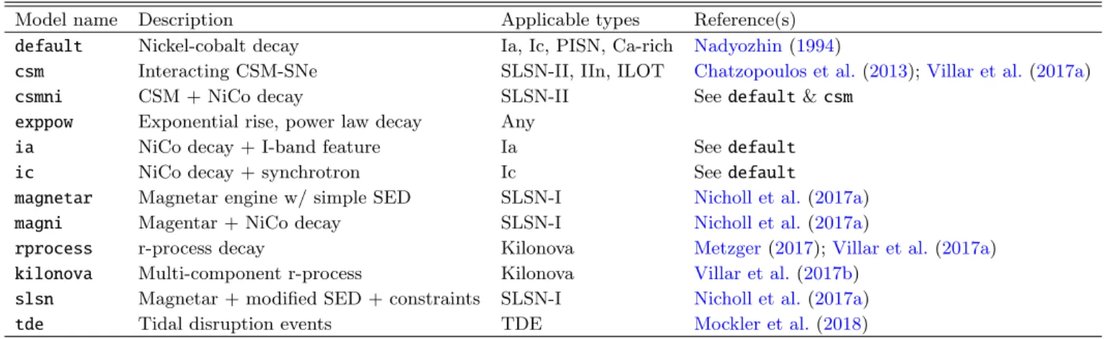
Table 1. Table of models currently available inMOSFiT.
Model name Description Applicable types Reference(s)
default Nickel-cobalt decay Ia, Ic, PISN, Ca-rich Nadyozhin(1994)
csm Interacting CSM-SNe SLSN-II, IIn, ILOT Chatzopoulos et al.(2013);Villar et al.(2017a)
csmni CSM + NiCo decay SLSN-II Seedefault&csm
exppow Exponential rise, power law decay Any
ia NiCo decay + I-band feature Ia Seedefault
ic NiCo decay + synchrotron Ic Seedefault
magnetar Magnetar engine w/ simple SED SLSN-I Nicholl et al.(2017a)
magni Magentar + NiCo decay SLSN-I Nicholl et al.(2017a)
rprocess r-process decay Kilonova Metzger(2017);Villar et al.(2017a) kilonova Multi-component r-process Kilonova Villar et al.(2017b)
slsn Magnetar + modified SED + constraints SLSN-I Nicholl et al.(2017a)
tde Tidal disruption events TDE Mockler et al.(2018)
• SEDs: Spectral energy distribution produced by a given component. A simple blackbody is a common assumption, but modified blackbodies and sums of blackbodies, or SEDs built from template spectra, can be yielded by these routines (at present, only simple and modified blackbodies are implemented). Extinction corrections from the host galaxy and the Milky Way are also applied here.
• Transforms: Temporal transformations of other functions of time yielded by a given component of a transient (the central engine, an intermediate re-processing zone, etc.), examples include reprocess-ing of the input luminosity through photon diffu-sion, or a viscous delay in the accretion of matter onto a central black hole.
• Utilities: Miscellaneous operators that don’t fall into the above categories. Examples include arith-metic operations upon the outputs from multiple input modules, which would be used for example to sum the energetic inputs of a magnetar and the decay of radioactive isotopes in a transient where both sources of energy are important.
4.3. Built-in models
Using the modules described above, a number of tran-sient models are constructed and included by default with MOSFiT (see Table 1). While several of the mod-els are good matches to the observed classes they rep-resent and have been extensively tested against data, speed considerations mandate that the models not be overly complex, with simple one-zone models represent-ing many of transients. Other models (such as the Ia model) serve as placeholders that only reproduce a given transient class’ basic properties, as specialty software ex-ists for these transients that are superior to MOSFiT’s model representations. For such transients it is likely that leveraging the collection of spectra on the Open As-tronomy Catalogs could yield better model matches, a
feature we expect to add in future versions of the code (see Section 7.4).
4.4. Modifying and creating models
In Table1, some of the models are combinations of two models (e.g., csmni) or simple additions to an existing model (e.g., ic). These models share much of the code and setup of the parent models from which they inherit, and indeed creating them often only involving proper modification of the appropriate JSONfile.
The first modification a user may wish to make is al-tering the priors on the given free parameters of a model. By modifying the prior class in the parametersJSONfile, a user for example might swap a flat prior in a parameter,
{ ... "vejecta":{ "min_value":5.0e3, "max_value":2.0e4 }, ... }
for a Gaussian prior provided by a separate observation,
{ ... "vejecta":{ "min_value":5.0e3, "max_value":2.0e4, "class":"gaussian", "mu":1.0e4, "sigma":1.0e3 }, ... }
Next, a user might consider altering which modules are executed in a given model, for example a user might wish
MOSFiT
to switch from a simple blackbody SED to a custom SED that better describes a transient’s spectral properties (as schematically shown in Figure 3). In this case, the user swaps a module (or modules) in the call stack in the model JSONfile, in this example from a blackbody
{ ... "blackbody":{ "kind":"sed", "inputs":[ "texplosion", "redshift", "densecore" ], "requests":{ "band_wave_ranges": "photometry" } }, "losextinction":{ "kind":"sed", "inputs":[ "blackbody", "nhhost", "rvhost", "ebv" ], "requests":{ "band_wave_ranges": "photometry" } }, ... }
to a custom SED function with a blackbody cutoff,
{ ... "blackbody_cutoff":{ "kind":"sed", "inputs":[ "texplosion", "redshift", "temperature_floor", "cutoff_wavelength" ], "requests":{ "band_wave_ranges": "photometry" } }, "losextinction":{ "kind":"sed", "inputs":[ "blackbody_cutoff", "nhhost",
Model A (Superluminous supernova) Transient data Free parameters Magnetar engine Photon diffusion Supernova photosphere Spectrum Photometry Score Priors Extinction Physics Model B (Kilonova) Transient data Free parameters r-process deposition Photon diffusion Kilonova photosphere Spectrum Photometry Score Priors Extinction Physics
Figure 3. Simplified schematic of two model trees con-structed in MOSFiT (not all modules shown, see Fig-ure 2 for an example of a full tree). The top model (Model A) shows a collection of modules appropriate for describing a superluminous supernova model, whereas the bottom panel shows a model appropriate for a kilo-nova, constructed by replacing modules in the superlumi-nous model (replaced modules shown in orange). In the schematic, green modules are inputs, blue modules pro-cess data from inputs and other modules, red modules are outputs, and the arrows connecting them indicate data exchange. "rvhost", "ebv" ], "requests":{ "band_wave_ranges": "photometry" } }, ... }
Note that in the above example the name of the mod-ule and everything that calls it (in this case just the
losextinction module) was altered to accommodate the new function.
Lastly, a user may find that none of the modules avail-able presently in MOSFiT are adequate for their needs,
for example if they wish to experiment with a new power source for a transient, and will create new ones to ad-dress them. In this case they can encode the required physics in a newPythonclass in the appropriate group-ing within the modules directory (see Section4.3), and add this module and its associated free parameters to the twoJSON files defining their model.
Writing new code for MOSFiT requires the most care on the part of the user, as they must be mindful that the sampling and optimization routines will always be limited by the execution time of a single model realiza-tion. The models that ship withMOSFiT are all compu-tationally simple and have sub-second execution times; more complicated models that may involve integrations of systems of differential equations that may take min-utes to execute per realization and thus will take that much longer when run within the MOSFiTframework.
4.5. Making models available to the community If a user wishes to share their model with a broader audience, the proper way to do so is to fork the MOSFiT
project, add their model and any supporting code, and submit that as a pull request. In general, it is the de-sire of the authors of this work that models contributed adhere to the following guidelines:
1. Parameters are preferred to be correspondent to physical properties of the transient, i.e. parameters like ejecta mass versus parameters like post-peak magnitude decline rate, although non-physical pa-rameters are sometimes appropriate for difficult-to-describe phenomena such as spectral line features. 2. Permit broad priors on their input parameters that remain physically reasonable to support the broad-est range of transients possible. Ideally, models should be capable of being applied to a broad range of transients, many of which they may fit poorly, and should extend beyond the present observed range of phenomenology to accommodate newly discovered extremal events. If a given combina-tion of parameters is known to be unphysical, the models should penalize those combinations via con-straints (see Section 4.2) rather than via narrow priors that might also excluded allowed portions of parameter space.
3. Models should utilize as much of the pre-existing modules as possible as opposed to creating their own separate stack of modules that they depend on. This reduces the number of unique points of failure for individual models.
By following these guidelines, we hope that models can be largely used “off the shelf” without modification by
the user, which means that a larger proportion of the provided model fits will originate from the same unique models that can be more directly compared, where model uniqueness is assessed as described in Section5.2. Exact adherence to these guidelines is notmandatory, and we are open to including models that may not fit exactly into our preferred mold.
5. INTERPRETING OUTPUTS
The way data is ingested by a program is only half of the way we interact with software, equally important is the way that software outputs its data and the ways that output can be used. In this section we describe some of the features MOSFiT provides to make its outputs as useful to the user as possible.
5.1. Sharing fits
As data reduction software evolves, and scientists move between institutions, sometimes original data can slip through the cracks. In order to preserve important re-search products, it is critical that data be shared in a way that it remains available indefinitely beyond its pro-duction date. The sharing of observational transient data has become increasingly common with public data repos-itories provided by space agencies (e.g. MAST, ESO), observing groups (e.g. the CfA, SNDB, Silverman et al. 2012), and third-party agglomerators (e.g. WISeREP, the OSC, SNaX, Yaron & Gal-Yam 2012; Guillochon et al. 2017; Ross & Dwarkadas 2017). But for models, the means to share results is extremely haphazard, with no standard mechanism for doing so.
In conjunction with the public release of the MOSFiT
software, the authors have extended the functionality of the Open Astronomy Catalogs to accommodate model fits. In addition to the observational data, the data pre-sented on the Open Astronomy Catalogs now contain the full model descriptions inMOSFiT’s model format, the pa-rameter combinations associated with each Monte Carlo realization, and light curves for all realizations, which are visually accessible on each modeled event’s page as shown in Figure 4. This data can be directly loaded by the user back into MOSFiT, where the user can rapidly reproduce the light curves with a different cadence, set of photometric bands, or variations on the inferred pa-rameters (see Section7.3).
5.2. Model uniqueness
A model can only be expected to be exactly repro-ducible if the code and data used to generate its output is identical. Because observing groups tend to operate independently from one another, the data fitted against from group to group is different in its time and frequency coverage, which can lead to different outcomes for pa-rameter inferences and forward modeling. Differences in
MOSFiT
Figure 4. Screenshot of figure presented on individ-ual event page for supernova LSQ12dlf (https://sne. space/sne/LSQ12dlf/). The observed data, shown by points, is displayed alongside Monte Carlo realizations of the light curve produced by aMOSFiT slsn run pub-lished in Nicholl et al. (2017a). A drop-down menu al-lows the user to select and display other model fits to the transient.
models used, even at the implementation level, such as the way an integration is performed, can also lead to real differences in outcome. Modest edits to model inputs such as changing the bounding range for a free parame-ter can also impact the score for a given model (or any proxy for it such as the WAIC, see Section6.3).
To ensure that users are comparing identical models to one another, MOSFiTcalculates three hashes for each fit before it is uploaded to the Open Astronomy Cat-alogs: a hash of the input data, a hash of the model dictionary, and a hash of the Python code invoked by that model. The hashes are generated by serializing the
JSON/Pythonfiles associated with the input/model/code into strings, which are then passed to the sha512 al-gorithm which generates the hash, of which the first 16 characters are stored. This means that any change to the input/model/code will result in a different hash output, which can be used to ensure that the same data and code were used to analyze a given event. As a simple example, consider the following event with a single observation,
{ "photometry":[ { "time":"55123.0", "magnitude":"13.63", "band":"V" } ] }
which yields a hash value of 1612F22510D5A407. Now assume that the photometry was later re-reduced and the magnitude has changed,
{ "photometry":[ { "time":"55123.0", "magnitude":"13.47", "band":"V" } ] }
this new data has a completely unique hash relative to the first,6B59BB401C31D86D. Together, these hashes help to reassure the user that the data and the model used to fit it are identical to what might have been produced by other users, and prevent inadvertent cross-model com-parisons. One remaining reproducibility concern that these hashes do not address are changes to the external packages that MOSFiT depends on, such as the outputs of variousSciPyroutines that may vary withSciPy ver-sion.
5.3. Choosing a Sampler and a Minimizer The biggest issue in Monte Carlo approaches is con-vergence; as these methods are stochastic, there is ab-solutely no guarantee that they will ever find the best solutions, nor properly describe the distributions of the posteriors, in the time allotted to them. MOSFiT em-braces a “grab-bag” approach of techniques to maximize the chances of a converged solution.
Because the modeling in MOSFiT is geared towards physical models of transients, as opposed to empirically-driven models, the evaluation of even simplistic semi-analytical models often requires the evaluation of mul-tiple levels of non-algebraic expressions. Whereas empirically-driven models are free to choose arbitrary analytical constructions (e.g. spline fits, combinations of power laws) that are easily differentiable, purely alge-braic representations of physical models are not usually possible. This means that any derivative expressions po-tentially required by the sampler/minimizer need to be constructed numerically. So long as the likelihood func-tion is smooth and continuous, these derivative can be approximated via finite differencing, but this is prone to error that can make methods that assume certain
constants of motion (e.g. Hamiltonian Monte Carlo, HMC) to fail to converge to the true global minimum and/or posterior (Betancourt 2017). The rewards how-ever are great if one is able to construct one’s problem into a framework where the derivatives can be calcu-lated in such a way that derivatives are well-behaved (e.g. Sanders et al. 2015b,a), which can yield performance that scales impressively even for problems with thousands of dimensions.
Unfortunately, little quantitative information can be gained about the transients from empirically-derived modeling alone without a concrete connection to the laws of physics. Ensemble samplers, such as the Goodman & Weare(2010) affine-invariance algorithm implemented byemcee (Foreman-Mackey et al. 2013), do not require any explicit derivative definition, and thus can be used in situations where the derivatives are not easily evaluated, and even in cases where a derivative is not even defin-able, as is the case for discretized parameters. However, it has been shown that such methods can take an exceed-ingly long time to converge to simple, well-behaved pos-terior functions if the number of dimensions m exceeds ∼ O(10) (Huijser et al. 2015). This makes the vanilla
emcee algorithm completely inappropriate for problems with m O(10), unless the function evaluations are cheap enough to run for many thousands of steps. It also suggests that caution should be exercised when inter-preting posterior distributions generated byemceewhen fitting models withm&O(10).
So which sampler is appropriate for modeling tran-sients? For modeling individual transients, the choice is in favor of ensemble-based methods for their simplic-ity and flexibilsimplic-ity, as physical models of transients are often able to successfully describe their bulk properties and make useful quantitative predictions even with mod-estm∼ O(10), a regime where ensemble-based methods can converge to the true posterior in a practical length of time. For hierarchical modeling of transients (Mandel et al. 2009,2011;Sanders et al. 2015a), which can involve thousands of free parameters, ensemble-based methods are likely not appropriate unless they are used in con-junction with other methods that improve their speed of convergence.
5.4. MOSFiT’s approach
The algorithmMOSFiTuses to advance walker positions is shown in Figure5. In this first release,MOSFiTuses the parallel-tempered version ofemceeas its main driver. As this algorithm has been shown to preserve detailed bal-ance, it is the only method employed to advance walker positions during the post-burn-in phase.
As the stretch-move suffers from slow convergence to the true solution in reasonably high-dimension problems, a pre-burn phase is performed that uses a variant of
emceewith a Gibbs-like stretch-move that doesnot pre-serve detailed balance. Rather than stepping in all di-mensions simultaneously, the Gibbs-like sampler at each step selects a random number of dimensions D to vary, where D ∈ [1−N], giving it more agility in the early phases where it can be easy for the walkers to become trapped in poor local minima. Once the pre-burn phase is completed, the algorithm reverts to the vanilla ensem-ble algorithm, the burn-in time of which has hopefully been reduced by the pre-burn procedure.
6. ASSESSING MODEL PERFORMANCE Goodness-of-fit can give us valuable information on a transient’s properties: it can quantitatively assess which combination of physical parameters reproduce a given event, and it can suggest to us which model is best repre-sentative of a given transient. In this section, we describe three error models: χ2
red minimization, maximum likeli-hood analysis, and Gaussian processes, all of which are available inMOSFiT(Gaussian process being the default). In much of the historical transient literature, goodness-of-fit has been assessed by either least squares (in cases where measurement errors are not known) or the reduced chi-square metric, χ2 red≡χ 2/N dof, where χ2= o X i=1 x2 i σ2 i , (1)
withxi≡Oi−Miis the difference between theith
obser-vationOiand model predictionMi(θ) respectively (θ
be-ing the free parameters),σiis the normal error of theith
observation (for reference, least squares would setσi = 1,
i.e. observational errors are ignored), Ndof =o−m is the degrees of freedom,o is the number of observations, and m is the number of free parameters in the model. Because of its simplicity, χ2red has been a favored met-ric when comparing models to one another. But there is danger in its simplicity: it assumes that the errors are best represented by Gaussian distributions of uncorre-lated noise, an assumption that is likely untrue for ob-servations in magnitude space and is especially inappro-priate for quantifying model errors, which are dominated by systematics. If the best possible model match yields a χ2
red 1, the transient is said to be underfitted by the model, suggesting that the model is incomplete, the errors in the data underestimated, or that the transient in question is better represented by different model. If the best possible match yields χ2
red1, that particular match is overfitted, suggesting the model has parame-ters that tune the model outputs but are not necessarily meaningful (e.g., an ad-hoc magnitude offset parameter), or that the errors in the data are overestimated, a less likely scenario than an underestimate given many diffi-cult to quantify sources of error.
MOSFiT 5. Repeat 1. Walk (Gibbs) 2. Select 4. Replace 3. Frack
Pre-burn Burn-in Output
6. Walk
7. Sample
Figure 5. Schematic representation of the algorithm inMOSFiTfor determining the parameter posterior distributions, where the cyan-colored regions indicate probability density of the likelihood function and the white circles represent walker positions. In a primary “pre-burn” phase, individual parameter combinations (“walkers”) are evolved using a Gibbs-like variant of the affine-invariant algorithm ofGoodman & Weare(2010) (Step 1), with walkers being selected (Step 2) periodically for optimization using SciPy’s global optimizers (Step 3), the results of which are substituted back into the walker ensemble (Step 4). This process is repeated (Step 5) for a predetermined number of cycles, after which the ensemble is evolved using the vanilla affine-invariant MCMC to ensure detailed balance (Step 6). Convergence is continuously checked using the Gelman-Rubin statistic (PSRF), which once satisfied triggers the collection of uncorrelated samples over the MC chain (Step 7), with sample frequency determined by the autocorrelation time.
Under the assumption that the simple error model adopted is correct, χ2red can be directly compared be-tween models (or different realizations of the same model), and all models with χ2
red . 1 are acceptable matches to a given transient. This means that even for different parameter combinations of the same model that there is no one “best” fit to a transient, and that all fits of comparable score should be presented alongside one another to gauge a model’s performance, with the fre-quency of a given combination depending on its likeli-hood: a Bayesian analysis. By considering all parameter combinations that are capable of matching a sequence of observations within a prescribed tolerance, parameter degeneracies can be identified by examining the resulting posteriors. These degeneracies can be used as a tool to determine how a model could potentially be improved: as an example, a hypothetical supernova model that finds that the progenitor mass and explosion energy parame-ters are strongly correlated would likely benefit from an improvement to the model, such as a more-detailed cal-culation of ejecta velocity based upon the star’s radial density profile.
So how does one select between two physically different models if both can yield model fits with χ2red.1? One heuristic approach that has been frequently employed is to favor the model with the lowest χ2
red, as it has the most tolerance to future changes to a model and/or data. But, under a Bayesian interpretation (with a suitably flat prior), the parameters associated with the fits of mini-mal χ2red belong to the region of parameter space for a
given model with the highest posterior probability den-sity, even if that region of parameter space is infinitesi-mally small. What is desired is actually the region oc-cupied by the majority of the probabilistic mass, which may span a much wider range of parameter combinations. Given that errors in model and data are likely underes-timated, even fits that yield “poor” χ2
red could still cor-respond to reality, a feature that must be marginalized over to correctly infer a transient’s parameters.
6.1. Identifying plausible matches
A better solution than identifying a single best fit is for the scientist to map all parameter combinations that yield plausible fits to their data. Once this map is com-pleted, the information content of the maps of multi-ple models can be compared using agreed-upon met-rics. In a Bayesian analysis, we identify all parame-ter combinations according to their posparame-terior probability, p(θ|O) ∝ p(O|θ)p(θ) (where p(θ) is the prior), rather than finding a single “best-fit” solution by minimizing theχ2 or maximizing the likelihoodp(O|θ).
One can perform a Bayesian analysis using reported measurement errors alone, in which case the likelihood is p(O|θ) ∝ exp(−χ2/2). However, when the mini-mum χ2
red 1, suggesting underestimated uncertain-ties, it is common to adopt an error model in which an additional variance σ2 is added to all measurement er-rors, representing an additional source of “white noise.” With this error model, the log likelihood is p(O|θ) =
Pn
i=1P(Oi|θ), where the likelihood of a single datum is
logp(O|θ) =−1 2 n X i=1 x2 i σ2+σ2 i + log 2π σ2+σ2i (2)
whereσ2is now included within the parameter vectorθ. Because the additional varianceσ2enters into both terms for logp, increasing its value both improves and penal-izes the score, resulting in a balance where the variance yielded by Bayesian analysis is the additional error re-quired to match the given model to the transient with χ2
red ' 1. Setting σ = 0 recovers a pure χ2red mini-mization (Equation (1)) inMOSFiT, which can be accom-plished via the command line (-F variance 0).
Is the source of this additional error from the observa-tions, or from the model, or both? Equation (2) assumes the additional error is normally distributed about the measurements and/or model (the additional errors could be viewed as coming from either, or both), a situation which could arise if, for example, the measurements have overestimated signal to noise ratios. For transient obser-vations, typical errors on measurements can vary wildly, with e.g. the best photometric measurements yielding errors at the millimag level. Aside from faint detections near the detection limit of a given instrument, the signal to noise of such observations is typically well estimated, and thus a major underestimate of normally distributed errors is unlikely. As photometry is performed relative to a set of standard stars, any additional error on top of the reported stochastic error is more likely to be system-atic, and is less often estimated and/or presented in the literature.
For semi-analytical models without a stochastic com-ponent, predictions can be exact to numerical precision, and thus all model errors are systematic and depend upon the level of accuracy prescribed by the computa-tion. This means that errors in a repeated measurement (say, observing a transient with a B-band filter) are likely to be strongly correlated over some timescale, and also correlated depending on the similarity of two observa-tions collected at the same time (e.g., the error in si-multaneous B- and g-band observations are likely to be strongly correlated). This serial correlationmeans that the additional error introduced by a model is poorly rep-resented by an additional error term that is normally distributed about the model mean. An error model that is more representative of serially correlated errors is thus desirable.
6.2. Gaussian processes
Error models that have become recent favorites are Gaussian processes, described in depth in Rasmussen & Williams (2006). Gaussian processes are a non-parametric method for fitting functions, and have broad
utility in their ability to provide continuous approxima-tions to time-series data, regardless of the underlying complexity. This makes them more amendable to so-lutions where the model and data can be different in a wider variety of ways, permitting wider deviance at par-ticular times and/or parpar-ticular frequencies along a given transient light curve. Gaussian processes are the default error model used in all of the transient models included withMOSFiT.
Gaussian processes describe the error using a covari-ance matrixKwhich contains entriesKij that are
pop-ulated by evaluating the kernel function for every pair of observed input coordinates i and j, from which the likelihood is computed via the expression
logp(O|θ) =−1 2x TK−1 ij x− 1 2log|Kij| − n 2log 2π, (3) where x is the vector of differences between model pre-dictions and observation. Note that Equation (3) reduces to Equation (2) if the off-diagonal terms inKij are set to
zero. A shortcut exists withinMOSFiTto zero out the off-diagonal terms via the command line (-F covariance). In MOSFiT the default kernel function is the squared exponential, which is defined by two lengthscales lt and
lλ, corresponding to the time between observations and
the difference in average wavelength between the filters used in those observations. With the difference in time lt,ij = ti −tj and average wavelength lλ,ij = ¯λi −λ¯j
between pairs of observations, the covariance matrix re-sulting from the application of this kernel is
Kij =σ2Kij,tKij,λ+σi2δij (4) Kij,t= exp − l2 t,ij 2lt2 ! (5) Kij,λ= exp − l2 λ,ij 2l2 λ ! (6) whereσ2is the extra variance (analogous to the variance in Equation (2)), σi is the observation error of the ith
observation, t is the time of observation, and λ is the mean wavelength of the observed band. The kernel is customizable by the user via the Kernel class, but we have found that this particular functional form works well for photometric time series. In the limit of lt and
lλapproaching zero, the GP likelihood becomes identical
to the simpler error model of Equation (2).
If a transient is poorly constrained, e.g. the number of observations is comparable to the number of model parameters, a bimodal distribution of solutions can be returned, where some of proposed solutions are “model-dominated”, and some solutions are “noise-dominated,” where the entirety of the time evolution of a given tran-sient is purely explained by random variation (see Sec-tion 5.4.1 and Figure 5.5 of Rasmussen & Williams
MOSFiT
2006)6. In such instances, the lengthscales will typically settle on values comparable to their upper bounds, which gives the noisy solution the latitude necessary to fit all variation over a transient’s full duration while still scor-ing relatively well. These noise-dominated solutions can often be fixated upon by the optimizer, as the average brightness of a transient can be achieved through a wide combination of physical parameters plus a long kernel length scale. In some cases the noise-dominated solution can actually perform better than a physical model; this is highly suggestive that the physical model used is not appropriate for a given transient.
6.3. Measure of total evidence for a model In order to evaluate the total evidence of a model with m free parameters, an m-dimensional integral must be performed over the full parameter space where the local likelihood is evaluated at every position. Unless the like-lihood function is analytic and separable, such an inte-gration is usually impossible to perform exactly, and can be prohibitive numerically without computationally eco-nomical sampling (e.g., nested sampling,Skilling 2004) or approximations (e.g., variation inference, Roberts et al. 2013).
In ensemble Monte Carlo methods like the one em-ployed by emcee, entire regions of the parameter space may remain completely unexplored, particularly if those regions have a low posterior density as compared to the region surrounding the global maximum. This means that the likelihood scores returned by the algorithm at individual walker locations cannot simply be added to-gether to determine the evidence for a model.
Instead, heuristic metrics or “information criteria” that correlate with the actual evidence can be used to evaluate models. These criteria typically relate the dis-tribution of likelihood scores to the overall evidence of a model, an indication of the fractional volume occu-pied by the ensemble of walkers. While multiple vari-ants of the criteria exist, a simple one to implement is the “Watanabe-Akaike information criteria” (Watanabe 2010;Gelman et al. 2014) or “widely applicable Bayesian criteria” (WAIC), defined as
WAIC = logp(O|θ)−var [logc p(O|θ)] (7) where p(O¯|θ) is the posterior sample mean of the like-lihood, andvar[logc p(O|θ)] is the posterior sample vari-ance of the log likelihood, using samples from the ensem-ble7.
6.4. Convergence
6 see also http://scikit-learn.org/stable/modules/
gaussian_process.html
7Note this differs by a factor -1 fromWatanabe(2010)’s original definition.
To be confident that a Monte Carlo algorithm has con-verged stably to the right solution, a convergence metric should be evaluated (and satisfied) before the evolution of a chain terminates. For ensemble-based approaches, the autocorrelation time has been suggested as a way to assess whether or not convergence has been achieved (Foreman-Mackey et al. 2013), and running beyond this time is a way to collect additional uncorrelated samples for the purpose of better resolving parameter posteriors. Ideally, a metric should inform the user how far away they are from convergence in addition to letting the user know when convergence has been achieved. In our test-ing, the autocorrelation time algorithm that ships with
emcee (acor) is susceptible to a number of edge cases that prevent it from executing successfully, which pro-vides the user with no information as to how close/far they are from reaching a converged state.
Instead of using this metric, we instead rely upon the “potential scale reduction factor” (PSRF, signified with
ˆ
R), also known as the Gelman-Rubin statistic (Gelman
& Rubin 1992), which measures how well-mixed a set of chains is over its evolution,
ˆ R =N+ 1 N ˆ σ2 + W − L−1 N L (8) ˆ σ2+=L−1 L W+ B L (9) B L = 1 N−1 N X j=1 ¯ θj.−θ¯.. 2 (10) W = 1 N(L−1) N X j=1 L X t=1 θjt−θ¯j. 2 , (11)
where N is the number of walker chains,L is the length of the chain,θjtis thetth value of a parameter in thejth
chain, ¯θj. is its sample mean in the jth chain, ¯θ.. is its
global sample mean over all chains,B/Lis the between-chain variance, and W is the within-chain variance. To calculate the PSRF for our multi-parameter models, we use the maximum of the PSRFs computed for each rameter, meaning our performance is gauged by the pa-rameter with the slowest convergence. As described in Brooks & Gelman (1998), a PSRF of 1.1 strongly sug-gests that the Monte Carlo chain has converged to the target distribution; we use this value asMOSFiT’s default when running until convergence using the -Rflag. Run-ning until convergence only guarantees that a single sam-pling (with size equal toN) can be performed, users who wish to produce more samples should use more chains or run beyond the time of convergence.
The primary advantage of the PSRF over the auto-correlation time is it is always computable, which gives the user some sense on how close a given run is to be-ing converged. In some instances, in particular if two
separate groups of walker chains are widely separated in parameter space, the PSRF may never reach the target value, this usually suggests the solution is multimodal and larger numbers of walkers should be used.
7. DISCUSSION 7.1. Stress Testing
With a standardized data format for transient data,
MOSFiT should be capable of yielding fits to any event provided in the Open Catalog format. To test this, we ran MOSFiTagainst the full list of SNe available on the Open Supernova Catalog with 5+ photometric measure-ments (∼16,000 SNe), and found that the code produced fits for all events without error. This demonstrated that
MOSFiT is robust despite the broad heterogeneity of the dataset, with the full list of SNe being composed of data constructed from observations collected from hundreds of different instruments.
7.2. Performance
Parameter inference where the number of parameters exceeds a few can be an expensive task, particularly when the objective function itself is expensive. In our testing, a few ten thousand iterations ofemcee are typically re-quired to produce posterior distributions in a converged state about the global maximum in likelihood space, with roughly ten times as many walkers as free parameters being recommended. As the models currently shipping with MOSFiT are mostly single-zone models with rela-tively cheap array operations, such runs can take any-where from a few hours (for events with dozens of detec-tions) to a few days (thousands of detecdetec-tions), with the wall time being reducible by runningMOSFiTin parallel. This performance is reasonable and comparable to sim-ilar Monte Carlo codes, but improvements to the core modules such as rewriting them in a compiled language could bring further performance improvements.
7.3. Synthetic Photometry
Once the ensembles of possible parameters have been determined for a given model,MOSFiTenables the user to generate synthetic photometric observations for any in-strument/band combination (Figure 6). In cases where a particular transient is not being modeled, a user may wish to generate these synthetic observations from a rea-sonable set of priors on the physical parameters, which could then be used to produce mock observations of pop-ulations of various transients, as is done in Villar et al. (2017a).
Alternatively, a user may wish to instead generate a light curve based upon the results of aMOSFiTrun. This might be done if a user wants to supplement the model outputs with additional data perhaps not provided by the
group that ran the original fit, such as the brightness in a particular band at a different set of epochs. If the model parameters and code are available, either via the Open Astronomy Catalogs or private exchange, the dataset can be loaded directly into MOSFiT via the -w flag, which loads data from a previousMOSFiTrun,
mosfit -e LSQ12dlf -w previous_run.json -i 0
where the -i 0 flag tells MOSFiT to regenerate its out-puts without evolving the walker positions. Adding to this command a few additional flags (such as the-Sflag, which adds more epochs between the first/last observa-tion, or the-Eflag, which extrapolates a number of days before/after the transient) permits the user to customize its output to their needs.
7.4. Future versions
While MOSFiT already implements many features re-quired of a code that ingests, processes, and produces transient data, there are several potential areas of im-provement to the code that would further enhance its utility. Below, we present our feature wish-list for future releases.
7.4.1. Flux and magnitude model matching
A majority of the transient literature, based on histor-ical precedent, presents observations in the form of mag-nitudes as opposed to fluxes. While magmag-nitudes have the advantage of being a logarithmic scale which can better display multiple orders of magnitude of evolution in brightness, the errors in magnitude space are asym-metric and non-Gaussian, especially as the observations approach the low signal-to-noise flux limit. For simplic-ity, MOSFiTcurrently yields magnitudes for the included models and compares those magnitudes to the observed values/errors, but eventually switching the model out-puts to flux space would confer several advantages, in-cluding more accurate upper limits and a less approx-imate Gaussian process error model that could utilize symmetrical errors.
7.4.2. Improved spectral modeling
For transients with hotter photospheres (e.g. tidal dis-ruption events, superluminous supernovae), the approx-imation of the SED as a blackbody or a sum of black-bodies still yields fairly accurate magnitude estimates for broadband filters. This assumption quickly breaks down for transients with cooler photosphere, a prime example being type Ia supernovae which have deep absorption lines even near maximum light (see e.g. Figure 1 of Sas-delli et al. 2016), which leads to large systematic color errors.
While detailed radiative transfer models can relate pa-rameters to output spectra (e.g. Boty´anszki & Kasen