Multi-model assessment of the impact of soil moisture initialization on mid-latitude 1
summer predictability 2
3
C. Ardilouze1*, L. Batté1, F. Bunzel2, D. Decremer3, M. Déqué1, F.J. Doblas-Reyes4,6, H.
4
Douville1, D. Fereday5, V. Guemas1,4, C. MacLachlan5, W. Müller2, C. Prodhomme4
5 6
1- CNRM-Météo France, Toulouse, France 7
2- Max Planck Institute for Meteorology, Hamburg, Germany 8
3- European Center for Medium range Weather Forecasts, Reading, United Kingdom 9
4- BSC-CNS, Barcelona, Spain 10
5- Met Office Hadley Centre, Exeter, United Kingdom 11
6- ICREA, Pg. Lluís Companys 23, 08010 Barcelona, Spain 12
13
* Corresponding Author: 14
Constantin Ardilouze ([email protected]), phone: +33(0) 561079912 15
16
Abstract: 17
Land surface initial conditions have been recognized as a potential source of predictability in 18
sub-seasonal to seasonal forecast systems, at least for near-surface air temperature prediction 19
over the mid-latitude continents. Yet, few studies have systematically explored such an influence 20
over a sufficient hindcast period and in a multi-model framework to produce a robust 21
quantitative assessment. Here, a dedicated set of twin experiments has been carried out with 22
boreal summer retrospective forecasts over the 1992-2010 period performed by five different 23
global coupled ocean-atmosphere models. The impact of a realistic versus climatological soil 24
moisture initialization is assessed in two regions with high potential previously identified as 25
hotspots of land-atmosphere coupling, namely the North American Great Plains and South-26
Eastern Europe. Over the latter region, temperature predictions show a significant improvement, 27
especially over the Balkans. Forecast systems better simulate the warmest summers if they 28
follow pronounced dry initial anomalies. It is hypothesized that models manage to capture a 29
positive feedback between high temperature and low soil moisture content prone to dominate 30
over other processes during the warmest summers in this region. Over the Great Plains, 31
however, improving the soil moisture initialization does not lead to any robust gain of forecast 32
quality for near-surface temperature. It is suggested that models biases prevent the forecast 33
systems from making the most of the improved initial conditions. 34
35
Keywords: 36
Land-surface initialization;seasonal forecasting;land-atmosphere coupling;multi-37
model;ensemble forecast 38
Acknowledgement : 39
The authors thank Jeff Knight (Met Office Hadley Centre) for his constructive comments on 40
earlier versions of this manuscript. The research leading to these results received funding from 41
the European Union Seventh Framework Programme (FP7/2007-2013) SPECS project (grant 42
agreement number 308378) and H2020 Framework Programme IMPREX project (grant 43
agreement number 641811). Constantin Ardilouze was also supported by the BSC Centro de 44
Excelencia Severo Ochoa Programme. 45
1 Introduction 46
47
Human activities are affected by climate-dependent factors, such as energy demand, crop yield 48
or disease risk management. This raises a growing demand for reliable and accurate sub-49
seasonal to seasonal forecasts of temperature and precipitation (Challinor et al. 2005, García-50
Morales et al. 2007, Thompson et al. 2006). Atmospheric predictability on these timescales is 51
mainly driven by the coupling between the atmosphere and slowly-evolving components of the 52
Earth system, such as the ocean, sea ice and land surfaces (Doblas-Reyes et al. 2013). Even if 53
tropical oceans provide the major source of global interannual variability through sea surface 54
temperature anomalies related to the El Niño Southern Oscillation (ENSO) phenomenon (Saha 55
et al. 2006, Stockdale et al. 2011), both observational and numerical studies have highlighted 56
the significant imprint of the continental surfaces on the climate system and their potential or 57
effective contribution to mid-latitude sub-seasonal to seasonal predictability, particularly for near-58
surface temperature (T2M) and precipitation. Among these components, snowpack (Dutra et al. 59
2011) and soil moisture anomalies (Seneviratne et al. 2010; Seneviratne et al. 2013) have been 60
the most investigated since they strongly affect the land surface energy budget and, hence, the 61
energy fluxes between the surface and the atmospheric boundary layer (Hirschi et al. 2011). 62
Land surface models (LSM), which have improved steadily in the past three decades, together 63
with increasing computational resources have allowed for more thorough studies and a better 64
understanding of the soil moisture and snow influence on the atmosphere at multiple spatio-65
temporal scales (Douville, 2010). A realistic snowpack initialization has been shown to be useful 66
both in boreal fall (e.g. Orsolini et al. 2013) and spring (e.g. Peings et al. 2011), when the 67
interannual variability of the Northern Hemisphere snow cover is relatively strong and has a 68
large impact on the surface energy budget given the available incoming solar radiation even at 69
high latitudes. 70
71
For summer predictions, the focus was mainly on soil moisture and its influence on near-surface 72
temperature and precipitation mainly via evapotranspiration. It has been demonstrated that soil 73
moisture content controls the evapotranspiration in regions with a semi-arid climate (“soil 74
moisture-limited regime”). In wet regions, the evapotranspiration rate mainly depends on 75
atmospheric control and not on soil water content (“energy-limited regime”). In the former, the 76
evaporative fraction modulated by soil moisture affects both the local water cycle (Dirmeyer 77
2006) and the surface energy balance, and hence temperature and precipitation (Dirmeyer et al. 78
2014, Koster et al. 2004b, Seneviratne et al. 2010). Additionally, soil moisture memory has 79
proven to last up to several months in some cases (Seneviratne et al. 2006, Orth and 80
Seneviratne, 2012, Hagemann and Stacke, 2015). Due to these characteristics, extreme warm 81
events can be triggered or at least amplified by dry soil initial conditions in terms of magnitude 82
(Fischer et al. 2007, Hirschi et al. 2011, Whan et al. 2015) and persistence (Lyon and Dole, 83
1995, Lorenz et al. 2010). 84
85
Previous studies have highlighted a number of “hotspots” where seasonal prediction skill can be 86
increased by realistic soil moisture initialization since they combine intense land-atmosphere 87
coupling processes with strong soil moisture persistence (Koster et al. 2004, Seneviratne et al. 88
2006, Dirmeyer et al. 2011). The North-American Great Plains and the region between the 89
Danube basin and the Mediterranean are often identified as belonging to these hotspots. Our 90
study will focus mainly on these two regions, namely the Southern Great Plains (SGP) and the 91
Balkan region (BKS). BKS and SGP boundaries are defined in Table 1 and highlighted by green 92
boxes in Figure 2. The second phase of the Global Land-Atmosphere Coupling Experiment 93
(GLACE-2, Koster et al. 2011), which consisted in a multi-model forecast quality assessment, 94
showed that a realistic soil moisture initialization provides significantly improved skill for air 95
temperature forecast up to two months ahead over the North American continent. More recent 96
studies confirmed this positive impact up to seasonal timescales (Materia et al. 2014, 97
Prodhomme et al. 2015). Prodhomme et al. (2015) described the benefits of soil initialization for 98
the quality of temperature predictions over large parts of Eastern Europe up to four month 99
forecast time. They could only achieve a successful hindcast of the summer of 2010 extreme 100
heat over western Russia with a realistic soil moisture initialization. 101
102
This study aims at exploring to what extent previous results are robust across a variety of 103
forecast systems. Its originality lies in being the first multi-model assessment of soil moisture 104
initialization impact on atmospheric predictability on seasonal timescales with ocean-105
atmosphere coupled models over a nearly two-decade period. We use a highly comprehensive 106
database of seasonal prediction experiments produced within the framework of the European 107
FP7 SPECS (Seasonal-to-decadal climate Prediction for the improvement of European Climate 108
Services) project and covering the 1992 to 2010 period. The following section describes the 109
forecast systems and datasets used to perform the experiments and to assess their output. 110
Section 3 focuses on the model systematic errors and on the predictive skill related to soil 111
moisture initialization. Section 4 explains how the models respond to the soil moisture 112
initialization over the two regions of interest (BKS and SGP) and precedes the discussion and 113
conclusions to this study in section 5. 114
115
2 Experimental design and methodology 116
117
2.1 Overview of the experiments 118
119
Five forecast systems (Table 2) have been used to perform twin sets of boreal summer season 120
hindcasts over the 1992-2010 period. These simulations start at the beginning of May and span 121
4 months, including the June-August trimester (JJA). 122
123
For each system, the twin experiments consist of one control and one sensitivity experiment 124
differing only by their land-surface initialization. The former is initialized with climatological 125
surface fields while the latter is performed with initial conditions closer to observed interannual 126
variations in soil moisture (hereafter ‘realistic’ initialization). The different strategies adopted to 127
derive these initial conditions are detailed in the following subsection. All the experiments 128
consist of 10-member ensemble simulations. The methods applied for the generation of the 129
ensembles as well as the experimental design are summarized in Table 2. 130
131
The five twin experiments allow the comparison of two fifty-member grand ensembles. They are 132
named ALL-CLIM and ALL-INIT hereafter. We refer similarly to CLIM and INIT experiments 133
when discussing individual forecast system results. The multi model approach diminishes the 134
impact of individual model errors and thus leads to more reliable seasonal predictions (Palmer 135
et al. 2004, Hagedorn et al. 2005). 136
2.2 Land-surface initial conditions 137
Different methods were used to generate the so-called ‘realistic’ initial conditions of soil moisture 138
used in the ALL-INIT ensemble: 139
- Atmosphere-Ocean General Circulation Model (AOGCM) 140
simulation relaxed towards reanalyses: 141
For MPI-ESM, divergence, vorticity, temperature and surface pressure were assimilated into the 142
atmospheric component (ECHAM6) and temperature, salinity and sea-ice concentration into the 143
ocean component (MPIOM). For data assimilation, ERA-Interim (hereafter ERAI, Dee et al. 144
2011) is used for the atmosphere, ORAS4 for the ocean and NSIDC/Bootstrap for sea ice. No 145
assimilation was performed in the LSM (JSBACH). 146
- Standalone LSM simulation forced by atmospheric reanalysis 147
This method was applied for the LSM component (JULES) of HADGEM3 applying WFDEI 148
atmospheric forcing. 149
- Land surface reanalysis dataset 150
The last three models used the pre-existing daily dataset of land surface pseudo-reanalysis 151
ERA-Interim/Land (hereafter ERALand, Balsamo et al. 2013). It results from a stand-alone run 152
of the HTESSEL LSM, forced by ERA-Interim atmospheric fields and bias-corrected 153
precipitation using the GPCP monthly climatology (Huffman et al. 2009) for precipitation. 154
The two AOGCMs using the HTESSEL land component (namely EC-Earth and ECMWF System 155
4) were initialized with May the 1st ERALand reanalyses, horizontally interpolated over the 156
model grid. For CNRM-CM5, ERALand data was additionally interpolated onto the SURFEX 157
vertical soil layers (which differ from the ERALand vertical distribution), while preserving the soil 158
wetness index for each soil layer (Boisserie et al. 2015). 159
160
These initial conditions were computed for the 1st of May start dates of each of the nineteen 161
years of the seasonal re-forecast experiments, e.g. 1992 through 2010. The land-surface initial 162
conditions for each of the five CLIM ensembles are obtained by averaging the initial conditions 163
for the 1st of May from the corresponding INIT initial conditions. 164
165
Snow initial conditions are also considered realistic with the described techniques to generate 166
INIT initial conditions. However, different choices have been made for CLIM : snow fields were 167
averaged for BSC-CLIM and MF-CLIM, similarly to soil moisture, while their yearly variability 168
was preserved in the other three CLIM simulations. This experimental set-up inhomogeneity 169
might affect the conclusions since significant snow-atmosphere coupling occurs during and after 170
snowmelt over snow transition zones of the Northern hemisphere (Xu and Dirmeyer, 2011). 171
However, this impact is considered limited in our regions of interest where the influence of snow 172
in boreal summer is lower than in other seasons. 173
2.3 Reference data and forecast quality assessment 174
The monthly-mean precipitation observations used are the Global Precipitation Climatology 175
Center (GPCC) (Schneider et al. 2008) gridded gauge analysis products, available at a 1º 176
resolution, while monthly mean T2M reference data are provided by the CRU TS v.3.23 analysis 177
(Harris et al. 2010). The ERA-Interim (Dee et al. 2011) dataset is used for daily averaged two-178
meter temperature as well as daily-mean precipitation and daily maximum and minimum 179
temperature (Tmax and Tmin, respectively) references as no other global daily precipitation or 180
temperature data spans the full hindcast period. Both observational and model outputs were re-181
gridded onto a T85 Gaussian grid and only land surface grid points are considered for score 182
computations. 183
184
The bias is computed as the mean difference between the model and the observed 185
climatologies. We assume that the individual model drift does not depend on the start dates, 186
meaning that no distinction between the different hindcast years is required to compute the 187
model climatologies. Removing the bias is equivalent to considering observed and re-forecast 188
anomalies relative to their respective climatologies. Thus, the skill of the simulation is evaluated 189
by means of the correlation coefficient (r) between the predicted and the observed anomalies of 190
a given variable. The difference rINIT minus rCLIM is computed at every grid point and then
191
mapped to highlight regions impacted by the land-surface initialization. 192
193
A confidence interval for correlations is provided by a 2-sided 95% confidence level t-test. The 194
assessment of correlation differences between the CLIM and INIT simulations must take into 195
account the degree of dependence between the two experiments as both are run over the same 196
time period. To that end, the Hotelling-Williams t-test is computed (Steiger, 1980). 197
In addition to correlation, the comparison of the root mean square error (RMSE) of each 198
experiment through the root mean square skill score (RMSSS) helps in assessing how the soil 199
moisture initialization affects the interannual departure from observations. The RMSSS, contrary 200
to the RMSE, is positively-oriented so that a negative (positive) score means the INIT ensemble 201
has lower (higher) skill than the CLIM ensemble. 202
203
RMSSS=1 - RMSE(INIT)/RMSE(CLIM) 204
205
The RMSSS is considered to be significantly different from 0 if RMSE(INIT) is not included into 206
the confidence interval of RMSE(CLIM) computed through a 95% confidence level chi2 test. 207 3 Results 208 3.1 Bias analysis 209 210
A preliminary analysis of the surface bias can provide insight on both individual and multi-model 211
climatological limitations, as well as an overview of the ensemble consistency. Biases are 212
estimated as the forecast-time dependent difference (temperature) or ratio (precipitation) 213
between ensemble mean and reference data. The bias analysis can also contribute to 214
understanding model differences in forecast skill. 215
216
This analysis reveals almost indistinguishable differences in pattern and amplitude between the 217
CLIM (Fig. S1) and INIT (Fig. 1) experiments for both T2M and precipitation fields. As expected, 218
soil initialization used in these experiments does not alter the model climate in the seasonal re-219
forecasts. 220
221
JJA precipitation and temperature biases from individual models show relatively inconsistent 222
patterns over Eurasia (Fig. 1). Over Eastern Siberia, the five models overestimate the amount of 223
rainfall, although the very limited number of rain gauges available in that region (Fig. S2b) 224
suggests that reference data may have a substantial level of uncertainty. Biases partly cancel 225
out in the multi-model over Central Europe, but a notable dry and warm bias over the Steppes 226
east of the Caspian Sea, and a strong wet bias over Eastern Russia and the Iberian Peninsula 227
tend to stand out of the multi-model ensemble average. For the latter region as well as for the 228
Steppes, since the observed amount of JJA precipitation is very low (Fig. S2a), small differences 229
between these values can result in a strong relative bias. Over North America, in contrast, all 230
models present fairly similar patterns of wet and slightly cold bias over Alaska and pronounced 231
dry and warm bias over the Central Plains. This warm bias was also found in many models of 232
the Coupled Model Intercomparison Project Phase 5 (CMIP5) and would stem from excessive 233
incoming shortwave radiation combined to a lack of evaporative fraction (Cheruy et al. 2014). 234
We will discuss further how this could impact the seasonal forecast quality with respect to soil 235
moisture initialization in section 4. This preliminary analysis confirms the interest of the multi-236
model approach since the individual model climatologies show a number of similarities with 237
each other and the multi-model biases are not excessively influenced by any one of the 238
contributing models. 239
240
Soil moisture biases are far more difficult to assess due to the scarcity of in-situ observations to 241
be assimilated in any soil moisture reanalysis. Furthermore, remote sensing can only reflect the 242
superficial soil layer state, without taking into account the deeper root-layer soil moisture, and 243
do not necessarily provide a sufficient sampling for deriving reliable monthly mean values. Root-244
zone soil moisture controls the plants’ transpiration and thereby plays a major influence on total 245
evapotranspiration in vegetated areas. Finally, the limited knowledge of soil depth and global 246
scale physical processes at stake leads to a large variety of land surface modelling techniques 247
and parameters, which somewhat hampers the inter-model comparison of soil moisture as well 248
as the comparison of simulated versus observed data. However, a straightforward way to gain 249
insight on the simulated soil moisture is to consider the total soil water content of the entire soil 250
depth averaged over specific regions for each model and to assess the relative evolution in time 251
of its daily climatology. This evolution can be compared with that of ERALand.The assessment 252
of the mean soil moisture over the SGP and BKS regions (Fig. S3) shows that the soil dries 253
faster than the reference for four models out of the five analysed over both regions, although 254
none of them shows any obvious abnormal evolution. However, for the SGP region, according 255
to ERALand, there is little evolution in the soil water content during the first third of the forecast 256
period, followed by a drying phase starting in mid-June. Only one forecast system evolves 257
similarly to ERALand during the steady stage but retains somewhat too much water afterwards. 258
The drying tendency occurs too early for the other systems. This suggests that in addition to the 259
JJA precipitation bias discussed earlier, these models simulate either a deficit of rain in May and 260
early June, or an excessive evapotranspiration, or both simultaneously. These results suggest 261
that understanding not just the model bias, but also the forecast drift is essential to have a 262
chance to correctly interpret the quality of a forecast system. 263
3.2 Summer skill over boreal mid-latitudes 264
Figure 2 shows the JJA seasonal anomaly correlations of ALL-CLIM and ALL-INIT for near 265
surface temperature. Large parts of continents south of 50º N show significant T2M correlation 266
in all the experiments. This feature could be attributed to the correct representation of ENSO 267
teleconnections by the models, but also to the warming trend over the recent period, especially 268
over Europe (Doblas-Reyes et al. 2013). These hypotheses are assessed by computing for 269
each grid point the temporal correlation of JJA simulated T2M with respectively JJA observed 270
T2M averaged over the Niño 3.4 region defined in Table 1 and JJA observed global T2M 271
averaged over land. ENSO teleconnections, if present, do not seem to impact greatly the skill 272
south of 50°N (Fig. S4a). Observations suggest that the models over-estimate the link between 273
Niño 3.4 and Eastern Canada T2M. However, T2M over Eastern Canada, Southern Greenland 274
and the Middle-East is significantly correlated with global T2M, with correlation values of similar 275
amplitude to the hindcast skill (Fig. S4b). This is supported by observations over the same 276
period (not shown) in addition to the longer 1979-2013 period (Fig S4d). On the contrary, the 277
interannual simulated T2M over BKS and SGP is not significantly correlated to the global T2M 278
during the hindcast period, meaning that the global warming trend does not account for most of 279
the skill found over these regions. This is further confirmed by removing a linear trend from both 280
experimental and reference data, which does not affect greatly the correlation pattern nor its 281
values (Fig. 3). 282
283
An overall increase of skill is found over Europe in the T2M correlation differences between INIT 284
and CLIM (Fig. 4a). ALL-INIT is only outperformed by ALL-CLIM over the Iberian Peninsula, 285
although not significantly, whereas the effect is either positive or neutral anywhere else. This 286
skill enhancement is significant over Scandinavia, Ukraine and most of the Balkans peninsula. 287
The assessment of the RMSSS computed with respect to the CLIM experiments (Fig. 4b) 288
confirms these improvements. Over North America, soil initialization leads to a limited score 289
improvement. The model even exhibits a significant decrease in skill over Central Canada. 290
However, it should be kept in mind that this region has a poor temperature skill in the first place. 291
Such upper latitude regions are considered to be in an energy-limited regime where the 292
evaporative fraction of the surface energy budget is not controlled by soil moisture. Moreover, 293
snow melting - soil freezing interactions within the HTESSEL model seem to generate too much 294
and early runoff, which could have implications on soil moisture storage after the melting season 295
(E. Dutra, personal communication). If this were the case, the May 1st land surface initial 296
conditions derived from ERALand, which are used for three models out of five, could then be 297
locally unsuitable. 298
299
The multi-model ALL-CLIM (Fig. S5) and ALL-INIT (Fig. 5) display almost no skill for 300
precipitation, except for Western North America. This could be related to the great influence of 301
the ENSO activity on the local atmospheric circulation, although evidence of this teleconnection 302
has been found mainly during the winter season (Quan et al. 2006, Yoon et al. 2015). This skill 303
pattern should be considered with caution as the region receives limited amounts of precipitation 304
during summer (Fig. S2), implying that correlation values may be influenced by extremely small 305
differences in precipitation amounts. The difference of skill computed between INIT and CLIM 306
for precipitation (Fig. 6a) is quite patchy over the Northern Hemisphere mid-latitudes. Moreover, 307
the Iberian Peninsula, which results as one of the very few regions where the increase of 308
correlation leads to significant predictive skill, receives limited amounts of rain in summer as 309
mentioned earlier. Hence, small changes in simulated precipitation may greatly impact 310
correlation values. The negligible improvement of RMSSS tends to support this hypothesis (Fig. 311
6b) although models have already exhibited skill for precipitation over this region in past 312
coordinated experiments (Diez et al. 2005) 313
314
The results described above suggest that the BKS region is one of the most positively impacted 315
by soil moisture initialization in terms of predictive skill for temperature. Furthermore, the multi-316
model ensemble displays relatively weak temperature and precipitation biases over BKS (Fig. 317
1), although one should keep in mind that some of the contributing models have pronounced 318
biases of opposite signs. On the other hand, SGP was previously identified as a region with a 319
high potential for seasonal predictability due to its sensitivity to soil moisture. This set of 320
experiments did not show any skill increase over SGP associated to improved land surface 321
initialization. A possible reason for this lack of sensitivity may be related to the common dry and 322
warm bias of the five individual models. 323
324
The next section of this paper therefore aims at providing insights on the reasons for such 325
contrasted results over SGP and BKS. This is achieved by comparing the relationship for these 326
two regions between the realistic initial soil moisture and the subsequent simulation of 327
temperature and precipitation during the hindcast period. The next section intends to shed light 328
on the link between the multi-model skill and the systematic error analysed so far. 329
4 Preliminary understanding of the models response to realistic soil moisture initialization 330
This section focuses on the two previously defined regions, namely BKS and SGP, to better 331
understand the response of seasonal predictions to soil moisture initial conditions. 332
333
The standard deviations of simulated JJA T2M anomalies over BKS and SGP are enhanced 334
with realistic initial conditions, especially over SGP (Table 3) confirming the sensitivity of the 335
models’ response to soil moisture conditions in summer. They also get closer to the observed 336
standard deviation value in each region. To assess this sensitivity more closely, temporal 337
correlations between detrended ERALand total soil water content at start dates and observed or 338
simulated JJA T2M have been computed (Table 4). The time series of these anomalies are 339
represented on Fig. 7 where the blue and red envelopes feature the temperature anomaly 340
spread between individual model ensemble means for respectively CLIM and INIT simulations. 341
In the following sections, both regions are analyzed separately. 342
4.1 SGP region 343
Over SGP, unlike in the observations, the simulated JJA T2M is significantly anticorrelated with 344
the initial soil moisture for the five models. This is well illustrated in Fig. 7 where prevailing dry 345
initial conditions in the early 2000’s coincide with warm simulated summers according to ALL-346
INIT, which does not match observations. This implies that models tend to overestimate either 347
the land-atmosphere coupling processes or their contribution among other factors that could 348
explain interannual near-surface temperature variability. 349
350
In order to provide further insight on the models’ response, 31-day running means of daily-351
averaged simulated fields are correlated with the initial soil water content on May 1st over the 352
re-forecast period. Results for temperature, precipitation and soil moisture according to the 353
forecast time throughout the four months of simulation are presented in Fig. 8. The initial soil 354
moisture is very persistent in the simulations, with a correlation coefficient close to 1 and barely 355
decreasing throughout the summer. This persistence is also present in the reference soil 356
moisture data, although less pronounced. This implies that initial dry (wet) anomalies in the 357
models rarely turn into wet (dry) anomalies during the summer, while such changes in sign are 358
marginally more likely in the reference data. When considering the INIT-ALL ensemble, initial 359
soil moisture is correlated with both simulated precipitation and Tmax over SGP from the 360
beginning of the period. This correlation grows stronger in time for a few days before reaching a 361
plateau for Tmax at about 0.9, i.e. about 80% of variance explained, while it is about 0.6, about 362
35% of variance explained, right from the start for precipitation and persists throughout the 363
whole summer. On the other hand, in the reference data, the correlations are of the same sign 364
as in the simulations but they are not significant and tend to zero after the first month for 365
temperature. This suggests a larger amount of intraseasonal variability in the observational 366
dataset that is not reproduced by the models. The latter tend to simulate a smoother evolution of 367
the variables. 368
369
Based on Seneviratne et al. (2010), the following mechanism could explain the simulated 370
tendencies. Years with initial dry soils lead to reduced evapotranspiration, which inhibits 371
precipitation and in turn increases soil dryness. As soil moisture decreases due to this positive 372
feedback loop, it fails to respond to the evaporative demand, permitting the role of the sensible 373
heat flux to grow in the surface energy budget, at the expense of the latent heat flux. This leads 374
to higher daily Tmax, which triggers another positive feedback loop by increasing evaporative 375
demand and thus reducing soil moisture content. At night, however, this mechanism is 376
weakened by the development of a stable boundary layer decoupling the land surface from the 377
atmosphere aloft. Based on an observational campaign over Kansas, Ha and Mahrt (2003) 378
highlighted the development of a surface inversion primarily due to radiative cooling when 379
turbulent fluxes collapse in the early evening. This could explain why simulated Tmin is not 380
significantly anticorrelated to initial soil moisture during the first days, unlike Tmax. However, the 381
anticorrelation becomes significant about two weeks later than for Tmax, ultimately reaching 382
values comparable to those of Tmax. This feature of INIT-ALL is supported by three individual 383
models but not by observations. The Tmin values are generally reached at the end of the night, 384
when the diurnal soil moisture-temperature feedback loop is still off. This lagged co-variability of 385
Tmin and soil moisture in the simulations could result from a progressive overall warming of the 386
surface-boundary layer system. Depending on the stability regime of the nocturnal boundary 387
layer over grassland (Mahrt 1999), turbulence due to wind shear at the top of the stable layer 388
may redistribute downward the heat stored in the residual layer aloft. This mechanism competes 389
with the suppression of turbulence by thermodynamic stability that favours nocturnal radiative 390
cooling of the surface (McNider et al. 2010). However, the representation of such complex 391
subgrid scale phenomena in large-scale GCMs is likely to be inadequate and a source of model 392
error. 393
394
It is beyond the scope of this study to determine the reasons for the discrepancies between the 395
coupled model simulations and the observations. However, the similarities between forecast 396
systems in terms of correlation between initial soil moisture and summer variables likely relate 397
to their similarities in terms of biases. If the simulated climate over SGP is too dry, as suggested 398
in section 3.1, the models' evapotranspiration remains strongly controlled by soil moisture but its 399
absolute value and variations are too small to impact climate variability (Seneviratne et al. 400
2010). An additional explanation can be provided by the development of the biases over SGP 401
during the forecast (Fig. 9). The simulated climatologies look smoother than for the reference 402
data because they result from a ten-member averaging. The comparison of the precipitation 403
daily climatologies (Fig. 9a) show that for four models out of five, the deficit of daily rainfall 404
establishes at the beginning of June and persists throughout summer. On the contrary, the 405
Tmax biases (Fig. 9b) develop at a different rate and reach different amplitudes among forecast 406
systems. Nonetheless, all of them switch from neutral or cold biases during the first month to 407
warm by the end of summer. In some cases, this warm systematic error starts to grow up to 408
forty days after the appearance of the precipitation bias. The contrast between simultaneous 409
precipitation biases and asynchronous temperature biases supports, albeit without confirming it, 410
the hypothesis that the majority of models have a limited capacity to represent accurate 411
precipitation in summer over this region. A number of studies suggest that summer precipitation 412
regime in that region has particular features that makes it very challenging to model properly. 413
These particularities are the atypical diurnal cycle of precipitation with a nocturnal maximum in 414
summer (Klein et al. 2006), the meso-scale systems that account for much of the warm season 415
precipitation (Mearns et al. 2012), or the atmospheric low-level jet that substantially contributes 416
to the moisture budget of this region and influences nocturnal convection triggering (Bellprat et 417
al., 2016). If confirmed, this dry bias would trigger the excessive soil drying and its reduced 418
ability to respond to the evaporative demand, eventually leading to the aforementioned 419
feedback loop with the atmosphere that amplifies temperature biases. 420
421
Tackling this bias issue seems to be a prerequisite for the forecast systems to make the most 422
out of the soil moisture initial conditions and thus to improve the prediction skill over SGP 423
Nonetheless, a dedicated study would be required to disentangle the role of the biases from that 424
of potential shortcomings in the simulated surface processes. 425
4.2 BKS region 426
Over BKS, the two hottest summers of the period, namely 2003 and 2007, had both drier initial 427
soil moisture conditions than average. These are correctly predicted only with the INIT 428
ensemble (Fig. 7). Similar results are found with the cooler than average summers of 1996, 429
1997 and 2006 despite wet initial anomalies of relatively low amplitude. Observations, as well as 430
the INIT multi-model ensemble, show significant correlation between the initial soil moisture and 431
summer T2M for the BKS region (Table 4). Yet, when considering the individual forecast 432
systems, no relationship could be established between this correlation and the gain of skill 433
permitted by land surface initialization over BKS (as shown in Figure S6). Hence, the increase in 434
T2M correlation related to land surface initialization in this region does not result from local 435
linear processes - such as persistence - derived from initial soil moisture anomalies. 436
437
A correlation analysis similar to that performed for the SGP region (Fig. 8) is displayed for the 438
BKS region on Figure 10. It shows very distinct correlation features among forecast systems. 439
The different systems do not highlight any common process that would help explaining the gain 440
of skill in this region. It is likely that a wider range of processes related to soil moisture coupling 441
with the atmosphere with contradictory effects are at play. As opposed to the SGP region, the 442
BKS region is characterized by a steep topography and the proximity of the sea. Based on 443
regional meso-scale simulations over France, Stéfanon et al. (2014) highlighted different soil 444
moisture-temperature responses over low-elevation plains, mountains and coastal regions 445
during heat waves. Over plains, the dominant mechanism is consistent with the positive 446
feedback loop described earlier. Over mountains, on the other hand, enhanced heat fluxes due 447
to dry anomalies can reinforce upslope winds and favor convective precipitation with a 448
subsequent cooling effect, hence a negative feedback. Dry anomalies can also enhance the 449
gradient of diurnal near surface temperature between the air above coastal land and sea. This 450
could trigger anomalous moist advection from the sea through the breeze process, resulting in a 451
negative feedback on T2M over land. These last two meso-scale mechanisms may compete 452
with the first one over BKS, in spite of the relatively low resolution of the models used. Since the 453
five forecast systems have quite distinct spatial resolutions, it is likely that the impact of these 454
mesoscale processes, if represented, differs greatly. 455
What could therefore explain the successful prediction of the hottest summers of 2003 and 2007 457
conditioned to realistic soil moisture initialization, as indicated by Fig.7 ? The study from Conil et 458
al. (2008) based on a single AGCM showed that the benefit of a realistic land surface 459
initialization for summer predictions appears when widespread and strong soil moisture 460
anomalies are observed at the beginning of the season. This result was found over typical land-461
atmosphere coupling hotspots, namely central North America and Eastern Europe. The present 462
work tends to generalize this result for the latter region when initial anomalies are negative. 463
Furthermore, Quesada et al. (2012) showed observational evidence of an asymmetry in hot day 464
predictability over Europe. Wet springs lead to a reduced number of hot summer days 465
regardless of the dominant large-scale weather pattern during summer, while dry springs 466
precede a greater number of hot days only if anticyclonic weather types prevail during the 467
summer. From these studies and our results, we can infer that initializing soil moisture 468
realistically is a necessary condition for models to predict abnormally warm summers, but not a 469
sufficient one. We hypothesize here that in the case of pronounced dry initial anomalies over the 470
BKS region, forecast systems agree on the dominant process of positive feedback between low 471
soil moisture, reduced fraction of latent heat flux and warmer temperature. However, as 472
mentioned earlier, verifying this statement would require additional studies with a dedicated 473
experiment framework. 474
5 Conclusion and Discussions 475
A set of multi-model seasonal prediction experiments aiming at assessing the impact of land 476
surface initial conditions on boreal summer predictability has been carried out in the framework 477
of the FP7-SPECS European project. Five distinct global coupled ocean-atmosphere forecast 478
systems were run with 10 members each, initialized on May 1st over the period 1992 to 2010 479
with climatological soil moisture conditions for the reference experiment, and realistic ones for 480
the sensitivity experiment. For both experiments, the 50 resulting members have been 481
considered together as a large multi-model ensemble. This is the first multi-model experiment 482
assessing the added-value of initializing the land surface in a ‘real’ prediction context, as 483
opposed to potential predictability and/or purely AGCM frameworks. It therefore provides the 484
most robust assessment of land surface initialization impact on boreal summer prediction quality 485
to date. The comparison of precipitation and near surface temperature scores show evidence of 486
an enhanced predictive skill over large parts of Europe for realistically versus climatologically 487
initialized simulations, although mainly for temperature and with a significant increase limited to 488
a few regions. No such conclusion can be drawn for Asia and North America. 489
490
Previous studies had identified several mid-latitude regions with a high summer prediction 491
potential a few months in advance, stemming from intense land-atmosphere coupling combined 492
with long-lasting soil moisture memory. Among them, the Balkans proved to actually gain 493
predictability from a more accurate soil moisture initialization, unlike the Southern Great Plains 494
of North America where no improvement was achieved.Over the latter region, the five models 495
show very similar overestimates of the correlation between initial soil moisture anomalies and 496
summer daily maximum temperature (Tmax) and daily mean precipitation with respect to the 497
correlation estimated from reference data. A locked positive feedback settles between dry (wet) 498
soil moisture anomalies leading to increased (decreased) Tmax and precipitation deficit, which 499
favours in turn an increase of the soil moisture anomaly. This overestimated feedback over SGP 500
is likely related to the systematic errors for temperature and precipitation, and in the excessive 501
decrease of soil water content during the early stage of the summer simulated by the majority of 502
forecast systems. Thus, biases appear as potential culprits in the lack of predictive skill 503
enhancement with respect to soil moisture initialization over SGP. Previous studies based on 504
CMIP experiments pointed out at model deficiencies in both cloud physics and 505
evapotranspiration processes that should be addressed over the Great Plains to reduce 506
systematic biases (Cheruy et al. 2014). 507
508
For the BKS region, the coupling of soil moisture with temperature and precipitation could be 509
driven by various processes with opposite feedbacks. Nonetheless, for some years with a 510
pronounced dry initial anomaly, summer predictions from distinct models agree on a warm JJA 511
T2M anomaly. It is likely that in the case of dry soil moisture anomalies combined with prevailing 512
anticyclonic weather regimes during summer such as Blocking or Atlantic Low (Quesada et al. 513
2012), the land-atmosphere coupling processes simulated by different models over BKS 514
converge towards a similar dominant process or feedback loop. 515
516
Previous studies suggested a potential remote impact of soil moisture initialization on summer 517
temperature prediction (Van den Hurk et al. 2012, Koster et al. 2014), that could be related to an 518
alteration of the atmospheric circulation either locally or remotely (Fischer et al. 2007). The 519
correlations between JJA T2M averaged over BKS and initial soil moisture computed on every 520
grid point for OBS and INIT (Fig. S7a) do not rule out such a hypothesis, since a few common 521
patterns appear such as high positive correlations over Northern Europe and negative 522
correlations East of the Black Sea. However these patterns are not large or significant enough 523
to conclude on this potential remote influence. 524
525
A limitation of this study stems from the discrepancies between experimental protocols for each 526
participating forecast system. For instance, it does not clearly disentangle the potential impact of 527
snowpack initial conditions as two contributors out of five averaged out snow cover parameters 528
in addition to soil moisture parameters to produce climatological initial conditions. According to 529
Xu and Dirmeyer (2011), the snow-atmosphere coupling strength can be considerable during 530
snowmelt and up to several weeks after that, due to the albedo and subsequent soil moisture 531
states. Even if the similarity of the models' response in this study suggests a limited impact in 532
our regions of interest, this pleads for a more careful assessment of snow cover and snow water 533
equivalent in the initial conditions of subseasonal to seasonal summer predictions. The diversity 534
of spatial resolution also hampers the investigation of potential physical processes at play. 535
Furthermore, our study does not take into account the proportion of the total soil water content 536
in models and in the reference data that is prone to imprint the atmosphere at seasonal scale by 537
means of evapotranspiration. A focus on the soil wetness index of the root layer instead of the 538
total soil water content is required to further disentangle the processes involved in the soil-539
moisture surface climate interplays and the associated predictability. The use of ERALand for 540
soil moisture initialization and as a reference data might be a source of uncertainties since no 541
in-situ nor remote-sensed soil observations are assimilated in this product. Nonetheless, state-542
of-the-art global remote sensed soil moisture products usually estimate superficial soil wetness. 543
Hirschi et al (2012) pointed out the limitations of a mere extrapolation of observed superficial 544
soil moisture to the root-zone and suggests an assimilation of these data in a land-surface 545
model to obtain a more realistic product. These limitations should be addressed when defining 546
the set-up of the predictability experiment of the Land Surface, Snow and Soil moisture Model 547
Intercomparison Project (LS3MIP, van den Hurk et al. 2016). 548
In the light of our results, two main topics would require future research and attention in the 550
community. The first one is that of the initialization technique, a potential caveat of this study. 551
The climatology and variability of distinct AOGCM land components may differ greatly because 552
of the diversity of parametrizations and the limited constraints with respect to the atmospheric 553
component. This questions the technique of initializing a model with data derived from another 554
model. However, even if the land initial conditions are computed from an offline simulation of the 555
same LSM that is then used in the coupled model simulation, initial shocks and spin-up may 556
occur due to inconsistencies at the land-atmosphere interface and ultimately degrade the 557
prediction skill. A cleaner initialization would imply to perform either a coupled data assimilation 558
or a coupled nudging towards observational data for each forecast system individually. 559
However, this technique does not explicitly correct the simulated precipitation, which can remain 560
biased and thus lead to an unrealistic soil water content. A correction of precipitation in this case 561
might jeopardize the water balance of the model. Therefore, the best initialization strategy is still 562
an open question, and may very well be model-dependent. 563
564
The role of vegetation and land-use on continental climate predictability is the second issue that 565
could be of great interest in future works. Previous studies have demonstrated that the use of 566
interactive vegetation affects precipitation variability (Alessandri and Navarra, 2008) as well as 567
T2M seasonal predictability over the continents (Weiss et al. 2012, Alessandri et al. 2016). The 568
extensive use of irrigation and crop growing practices can affect water fluxes between the soil 569
and the atmosphere. Mueller et al (2015) showed evidence that agricultural intensification - and 570
to a lesser extent increased irrigation - over the past century led to cooler temperature 571
extremes and enhanced rainfall during the growing season in the North American Midwest. 572
These features are not taken into account in the coupled models used in this paper whereas 573
they affect atmospheric observations assimilated in the reference data. The results of the 574
present study plead for a coordinated seasonal prediction effort aiming at enlightening the 575
impact of vegetation and land-use on summer predictive skill over mid-latitudes. 576
577
References 578
Alessandri A, Navarra A (2008) On the coupling between vegetation and rainfall inter-annual 579
anomalies: Possible contributions to seasonal rainfall predictability over land areas. Geophys 580
Res Lett. doi: 10.1029/2007gl032415 581
Alessandri A, Catalano F, De Felice M, Van Den Hurk B, Doblas Reyes FJ ,Boussetta S, 582
Balsamo G, Miller P (2016) Multi-scale enhancement of climate prediction over land by 583
increasing the model sensitivity to vegetation variability in EC-Earth. Clim Dyn, In Press. 584
Baehr J, Piontek R (2014) Ensemble initialization of the oceanic component of a coupled model 585
through bred vectors at seasonal-to-interannual timescales. Geosci Model Dev 7:453–461. doi: 586
10.5194/gmd-7-453-2014 587
Balsamo G, Albergel C, Beljaars A et al (2015) ERA-Interim/Land: a global land reanalysis 588
dataset. Hydrol Earth Syst Sci 19:389-407. doi: 10.5194/hess-19-389-2015 589
Bellprat O, Kotlarski S, Lüthi D et al. (2016). Objective calibration of regional climate models: 590
Application over Europe and North America. J Climate, 29(2), 819-838. doi: 10.1175/JCLI-D-15-591
0302.1 592
Best MJ, Pryor M, Clark DB, et al (2011) The Joint UK Land Environment Simulator (JULES), 593
Model description – Part 1: Energy and water fluxes. Geosci Model Dev Discuss 4:595–640. 594
doi: 10.5194/gmdd-4-595-2011 595
Boisserie M, Decharme B, Descamps L, Arbogast P (2016) Land surface initialization strategy 596
for a global reforecast dataset. QJR Meteorol Soc 142:880–888. doi: 10.1002/qj.2688 597
Boussetta S, Balsamo G, Beljaars A et al (2012) Natural land carbon dioxide exchanges in the 598
ECMWF integrated forecasting system: implementation and offline validation. European Centre 599
for Medium-Range Weather Forecasts, Shinfield Park, Reading 600
Challinor AJ, Slingo JM, Wheeler TR, Doblas-Reyes FJ (2005) Probabilistic simulations of crop 601
yield over western India using the DEMETER seasonal hindcast ensembles. Tellus A 57:498– 602
512. doi: 10.1111/j.1600-0870.2005.00126.x 603
Cheruy F, Dufresne JL, Hourdin F, Ducharne A (2014) Role of clouds and land-atmosphere 604
coupling in midlatitude continental summer warm biases and climate change amplification in 605
CMIP5 simulations. Geophys Res Lett, 41, 6493–6500, doi:10.1002/2014GL061145. 606
Conil S, Douville H, Tyteca S (2008) Contribution of realistic soil moisture initial conditions to 607
boreal summer climate predictability. Clim Dyn 32:75–93. doi: 10.1007/s00382-008-0375-9 608
Dee DP, Uppala SM, Simmons AJ et al (2011) The ERA-Interim reanalysis: configuration and 609
performance of the data assimilation system. QJR Meteorol Soc 137:553–597. doi: 610
10.1002/qj.828 611
Díez E, Primo C, García-Moya JA, Gutiérrez JM et al (2005), Statistical and dynamical 612
downscaling of precipitation over Spain from DEMETER seasonal forecasts. Tellus A, 57: 409– 613
423. doi:10.1111/j.1600-0870.2005.00130.x 614
Dirmeyer PA (2006) The Hydrologic Feedback Pathway for Land–Climate Coupling. J 615
Hydrometeor 7:857–867. doi: 10.1175/jhm526.1 616
Dirmeyer PA (2011) The terrestrial segment of soil moisture-climate coupling. Geophys Res Lett. 617
doi: 10.1029/2011gl048268 618
Dirmeyer PA, Wang Z, Mbuh MJ, Norton HE (2014) Intensified land surface control on boundary 619
layer growth in a changing climate. Geophys Res Lett 41:1290-1294, doi: 620
10.1002/2013GL058826 621
Doblas-Reyes FJ, García-Serrano J, Lienert F et al (2013) Seasonal climate predictability and 622
forecasting: status and prospects. WIREs Clim Change 4:245–268. doi: 10.1002/wcc.217 623
Douville H (2009) Relative contribution of soil moisture and snow mass to seasonal climate 624
predictability: a pilot study. Clim Dyn 34:797–818. doi: 10.1007/s00382-008-0508-1 625
Dutra E, Schär C, Viterbo P, Miranda PMA (2011) Land-atmosphere coupling associated with 626
snow cover. Geophys Res Lett. doi: 10.1029/2011gl048435 627
Fischer EM, Seneviratne SI, Vidale PL et al (2007) Soil Moisture–Atmosphere Interactions 628
during the 2003 European Summer Heat Wave. J Climate 20:5081–5099. doi: 629
10.1175/jcli4288.1 630
García-Morales MB, Dubus L (2007) Forecasting precipitation for hydroelectric power 631
management: how to exploit GCM's seasonal ensemble forecasts. Int J Climatol 27:1691–1705. 632
doi: 10.1002/joc.1608 633
Ha KJ and Mahrt L (2003). Radiative and turbulent fluxes in the nocturnal boundary layer. Tellus 634
A, 55(4), 317-327.doi:10.1034/j.1600-0870.2003.00031.x 635
Hagedorn R, Doblas-Reyes FJ, Palmer TN (2005) The rationale behind the success of multi-636
model ensembles in seasonal forecasting - I. Basic concept. Tellus A 57:219–233. doi: 637
10.1111/j.1600-0870.2005.00103.x 638
Hagemann S, Stacke T (2014) Impact of the soil hydrology scheme on simulated soil moisture 639
memory. Clim Dyn 44:1731–1750. doi: 10.1007/s00382-014-2221-6 640
Harris I, Jones P, Osborn T, Lister D (2013) Updated high-resolution grids of monthly climatic 641
observations - the CRU TS3.10 Dataset. Int J Climatol 34:623–642. doi: 10.1002/joc.3711 642
Hazeleger W, Wang X, Severijns C et al (2011) EC-Earth V2.2: description and validation of a 643
new seamless earth system prediction model. Clim Dyn 39:2611–2629. doi: 10.1007/s00382-644
011-1228-5 645
Hirschi M, Seneviratne SI, Alexandrov V et al (2010) Observational evidence for soil-moisture 646
impact on hot extremes in southeastern Europe. Nature Geosci 4:17–21. doi: 647
10.1038/ngeo1032 648
Hirschi M, Mueller B, Dorigo W, Seneviratne S (2014) Using remotely sensed soil moisture for 649
land–atmosphere coupling diagnostics: The role of surface vs. root-zone soil moisture variability. 650
Remote Sensing of Environment 154:246–252. doi: 10.1016/j.rse.2014.08.030 651
Huffman GJ, Adler RF, Bolvin DT, Gu G (2009) Improving the global precipitation record: GPCP 652
Version 2.1. Geophys Res Lett. doi: 10.1029/2009gl040000 653
Hurk BVD, Doblas-Reyes F, Balsamo G et al (2010) Soil moisture effects on seasonal 654
temperature and precipitation forecast scores in Europe. Clim Dyn 38:349–362. doi: 655
10.1007/s00382-010-0956-2 656
Hurk BVD, Kim H, Krinner G et al (2016) The Land Surface, Snow and Soil moisture Model 657
Intercomparison Program (LS3MIP): aims, set-up and expected outcome. Geosci Model Dev 658
Discuss 1–41. doi: 10.5194/gmd-2016-72 659
Klein SA, Jiang X, Boyle J, Malyshev S, Xie S (2006) Diagnosis of the summertime warm and 660
dry bias over the U.S. Southern great plains in the GFDL climate model using a weather 661
forecasting approach. Geophys. Res. Lett. 33 :L18805.doi:10.1029/2006gl027567 662
Koster RD (2004) Regions of Strong Coupling Between Soil Moisture and Precipitation. Science 663
305:1138–1140. doi: 10.1126/science.1100217 664
Koster RD, Sud YC, Guo Z et al (2006) GLACE: The Global Land–Atmosphere Coupling 665
Experiment. Part I: Overview. J Hydrometeor 7:590–610. doi: 10.1175/jhm510.1 666
Koster RD, Chang Y, Schubert SD (2014) A Mechanism for Land–Atmosphere Feedback 667
Involving Planetary Wave Structures. J Climate 27:9290–9301. doi: 10.1175/jcli-d-14-00315.1 668
Ma H-Y, Xie S, Klein SA et al (2014) On the Correspondence between Mean Forecast Errors 669
and Climate Errors in CMIP5 Models. J Climate 27:1781–1798. doi: 10.1175/jcli-d-13-00474.1 670
Maclachlan C, Arribas A, Peterson KA et al (2014) Global Seasonal forecast system version 5 671
(GloSea5): a high-resolution seasonal forecast system. QJR Meteorol Soc 141:1072–1084. doi: 672
10.1002/qj.2396 673
Mahrt L (1999) Stratified Atmospheric Boundary Layers. Boundary-Layer Meteorology 90: 375-674
396. doi:10.1023/A:1001765727956 675
Masson V, Moigne PL, Martin E et al (2013) The SURFEXv7.2 land and ocean surface platform 676
for coupled or offline simulation of earth surface variables and fluxes. Geosci Model Dev 6:929– 677
960. doi: 10.5194/gmd-6-929-2013 678
Materia S, Borrelli A, Bellucci A et al (2014) Impact of Atmosphere and Land Surface Initial 679
Conditions on Seasonal Forecasts of Global Surface Temperature. J Climate 27:9253–9271. 680
doi: 10.1175/jcli-d-14-00163.1 681
Lyon B, Dole RM (1995) A Diagnostic Comparison of the 1980 and 1988 U.S. Summer Heat 682
Wave-Droughts. J Climate 8:1658–1675. doi: 10.1175/1520-683
0442(1995)008<1658:ADCOTA>2.0.CO;2 684
McNider RT, Christy JR, Biazar A (2010) A stable boundary layer perspective on global 685
temperature trends IOP Conf. Ser.: Earth Environ. Sci. 13 012003 doi: 10.1088/1755-686
1315/13/1/012003 687
Mearns LO, Arritt R, Biner S, et al.(2012) The North American Regional Climate Change 688
Assessment Program: Overview of Phase I Results. Bull. Amer. Meteor. Soc., 93, 1337–1362, 689
doi: 10.1175/BAMS-D-11-00223.1. 690
Mueller ND, Butler EE, Mckinnon KA et al (2015) Cooling of US Midwest summer temperature 691
extremes from cropland intensification. Nature Climate Change 6:317–322. doi: 692
10.1038/nclimate2825 693
Orsolini YJ, Senan R, Balsamo G et al (2013) Impact of snow initialization on sub-seasonal 694
forecasts. Clim Dyn 41:1969–1982. doi: 10.1007/s00382-013-1782-0 695
Orth R, Seneviratne SI (2012) Analysis of soil moisture memory from observations in Europe. J 696
Geophys Res. doi: 10.1029/2011jd017366 697
Peings Y, Douville H, Alkama R, Decharme B (2010) Snow contribution to springtime 698
atmospheric predictability over the second half of the twentieth century. Clim Dyn 37:985–1004. 699
doi: 10.1007/s00382-010-0884-1 700
Prodhomme C, Doblas-Reyes F, Bellprat O, Dutra E (2015) Impact of land-surface initialization 701
on sub-seasonal to seasonal forecasts over Europe. Clim Dyn. doi: 10.1007/s00382-015-2879-4 702
Quan X, Hoerling M, Whitaker J et al (2006) Diagnosing Sources of U.S. Seasonal Forecast 703
Skill. J Climate 19:3279–3293. doi: 10.1175/jcli3789.1 704
Quesada B, Vautard R, Yiou P et al (2012) Asymmetric European summer heat predictability 705
from wet and dry southern winters and springs. Nature Climate Change 2:736–741. doi: 706
10.1038/nclimate1536 707
Raddatz TJ, Reick CH, Knorr W et al (2007) Will the tropical land biosphere dominate the 708
climate–carbon cycle feedback during the twenty-first century? Clim Dyn 29:565–574. doi: 709
10.1007/s00382-007-0247-8 710
Saha S, Nadiga S, Thiaw C et al (2006) The NCEP Climate Forecast System. J Climate 711
19:3483–3517. doi: 10.1175/jcli3812.1 712
Schneider U, Fuchs T, Meyer-Christoffer A, Rudolf B. (2008). Global precipitation analysis 713
products of the GPCC. Global Precipitation Climatology Centre (GPCC), DWD, Internet 714
Publikation, 112. ftp://ftp.dwd.de/pub/data/gpcc/PDF/GPCC_intro_products_2008.pdf. Accessed 715
May 25th 2016 716
Seneviratne SI, Lüthi D, Litschi M, Schär C (2006) Land–atmosphere coupling and climate 717
change in Europe. Nature 443:205–209. doi: 10.1038/nature05095 718
Seneviratne SI, Corti T, Davin EL et al (2010) Investigating soil moisture–climate interactions in 719
a changing climate: A review. Earth-Science Reviews 99:125–161. doi: 720
10.1016/j.earscirev.2010.02.004 721
Seneviratne SI, Wilhelm M, Stanelle T et al (2013) Impact of soil moisture-climate feedbacks on 722
CMIP5 projections: First results from the GLACE-CMIP5 experiment. Geophys Res Lett 723
40:5212–5217. doi: 10.1002/grl.50956 724
Stéfanon M, Drobinski P, D’Andrea F et al (2013) Soil moisture-temperature feedbacks at meso-725
scale during summer heat waves over Western Europe. Clim Dyn 42:1309–1324. doi: 726
10.1007/s00382-013-1794-9 727
Steiger JH (1980) Tests for comparing elements of a correlation matrix. Psychological Bulletin 728
87:245–251. doi: 10.1037/0033-2909.87.2.245 729
Stevens B, Giorgetta M, Esch M et al (2013) Atmospheric component of the MPI-M Earth 730
System Model: ECHAM6. J Adv Model Earth Syst 5:146–172. doi: 10.1002/jame.20015 731
Stockdale TN, Anderson DLT, Balmaseda MA et al (2011) ECMWF seasonal forecast system 3 732
and its prediction of sea surface temperature. Clim Dyn 37:455–471. doi: 10.1007/s00382-010-733
0947-3 734
Thomson MC, Doblas-Reyes FJ, Mason SJ et al (2006) Malaria early warnings based on 735
seasonal climate forecasts from multi-model ensembles. Nature 439:576–579. doi: 736
10.1038/nature04503 737
Voldoire A, Sanchez-Gomez E, Mélia DSY et al (2012) The CNRM-CM5.1 global climate model: 738
description and basic evaluation. Clim Dyn 40:2091–2121. doi: 10.1007/s00382-011-1259-y 739
Waters J, Lea DJ, Martin MJ et al (2014) Implementing a variational data assimilation system in 740
an operational 1/4 degree global ocean model. QJR Meteorol Soc 141:333–349. doi: 741
10.1002/qj.2388 742
Weedon GP, Balsamo G, Bellouin N et al (2014) The WFDEI meteorological forcing data set: 743
WATCH Forcing Data methodology applied to ERA-Interim reanalysis data. Water Resour Res 744
50:7505–7514. doi: 10.1002/2014wr015638 745
Weiss M, Hurk BVD, Haarsma R, Hazeleger W (2012) Impact of vegetation variability on 746
potential predictability and skill of EC-Earth simulations. Clim Dyn 39:2733–2746. doi: 747
10.1007/s00382-012-1572-0 748
Whan K, Zscheischler J, Orth R et al (2015) Impact of soil moisture on extreme maximum 749
temperatures in Europe. Weather and Climate Extremes 9:57–67. doi: 750
10.1016/j.wace.2015.05.001 751
Xu L and Dirmeyer P (2011) Snow-atmosphere coupling strength in a global atmospheric model, 752
Geophys Res Lett 38, L13401, doi:10.1029/2011GL048049 753
Yoon J-H, Leung LR (2015) Assessing the relative influence of surface soil moisture and ENSO 754
SST on precipitation predictability over the contiguous United States. Geophys Res Lett 755
42:5005–5013. doi: 10.1002/2015gl064139 756
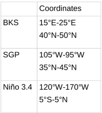
Tables 757 758 Coordinates BKS 15°E-25°E 40°N-50°N SGP 105°W-95°W 35°N-45°N Niño 3.4 120°W-170°W 5°S-5°N
Table 1: Boundary coordinates of the BKS, SGP and Niño 3.4 boxes 759
760
Exp. Name Model Horizontal Resolution
Vertical levels Ensemble generation Land surface component Land surface initialization Atmosphere, ocean and sea-ice initializations MPI-CLIM MPI-INIT MPI-ESM v.1.1.00 (Stevens et al., 2013) Atm/Land:T63 (~300 km) Ocean: GR15 (two poles in Greenland / Antarctica, 1.5 degree resolution) Atm: 47 Ocean: 40 Atm: slight disturbance of stratospheric diffusion Ocean: breeding vectors (Baehr & Piontek, 2014) JSBACH (Raddatz et al., 2007) GCM run with nudging of the atmosphere, superficial ocean and sea-ice towards reanalyses (resp. ERAI, ORAS4 and NSIDC) atm:ERAI ocean:ORAS4 sea-ice:NSIDC EC-CLIM EC-INIT
ECMWF Sys4 Atm/Land: N128 (TL255, ~80km) Ocean: NEMO ORCA 1° L42 Atm: 91 Ocean: 42
singular vectors CHTESSEL-Lakes (Boussetta et al. 2012) ERALand horizontal interpolation (same model) Atm: ERAI Ocean: ORAS4 MF-CLIM MF-INIT CNRM-CM5 (Voldoire et al. 2013 Atm/Land: Tl127 (~150 km) Ocean: NEMO Orca 1º L42 Atm: 91 Ocean: 42 Initial atmospheric perturbations SURFEX V7.2 (Masson et al. 2012) ERALand horizontal and vertical interpolation with conservative Total Soil Wetness Index (different model) Atm: ERAI Ocean: ORAS4 Sea-ice: restarts from a nudged run BSC-CLIM BSC-INIT EC-Earth V2.3 (Hazeleger et al. 2012) Atm/Land: T106 (~120km) Ocean: NEMO Orca 1° Atm: 91 Ocean: 46 Singular vectors in the atmosphere; different members of ORAS4 reanalyses for the ocean HTESSEL ERALand horizontal interpolation (same model) Atm: ERAI Ocean: ORAS4 Sea-ice: IC3 analysis MO-CLIM MO-INIT GloSea5 (Maclachlan et al., 2015) Atm/Land: N216 (~50km) Ocean: ORCA 0.25° Atm : 85 Ocean:75 Lagged start dates and SKEB stochastic physics scheme JULES (Best et al., 2011) JULES offline run driven with WFDEI atmospheric data (Weedon et al., 2014)
Atm: ERAI Ocean and sea-ice: GloSea5 reanalysis (Waters et al., 2015
Table 2: Summary of the simulations 761
762
BKS SGP
OBS 0.69 1.01
ALL-CLIM 0.40 0.51
ALL-INIT 0.50 0.88
Table 3: Standard deviation of JJA area-averaged T2M anomaly (K)
BKS SGP OBS -0.58* 0.18 ALL-INIT -0.50* -0.64* MPI-INIT -0.46* -0.53* MO-INIT -0.71* -0.6* MF-INIT -0.35 -0.53* EC-INIT -0.23 -0.48* BSC-INIT -0.20 -0.55*
Table 4: Anomaly correlations of detrended ERALand May 1st total soil moisture with detrended area-averaged June-to-August T2M. 95% confidence significant values are marked by a star