Composite likelihood for multiple multistate processes

(1)

Composite likelihood for joint analysis of multiple multistate

processes via copulas

LIQUN DIAO

Department of Biostatistics and Computational Biology

,

University of Rochester Medical Center, Rochester, NY, 14642, United States Liqun [email protected]

RICHARD J. COOK

Department of Statistics and Actuarial Science, University of Waterloo, Waterloo, ON, N2L 3G1, Canada

Summary

A copula-based model is described which enables joint analysis of multiple progressive multi-state processes. Unlike intensity-based or frailty-based approaches to joint modeling, the copula formulation proposed herein ensures that a wide range of marginal multistate processes can be specified and the joint model will retain these marginal features. The copula formulation also facilitates a variety of approaches to estimation and inference including composite likelihood and two-stage estimation procedures. We consider processes with Markov margins in detail, which are often suitable when chronic diseases are progressive in nature. We give special attention to the setting in which individuals are examined intermittently and transition times are consequently interval-censored. Simulation studies give empirical insight into the different methods of analysis and an application involving progression in joint damage in psoriatic arthritis provides further illustration.

Keywords: composite likelihood, copula model, interval censoring, Markov process, multiplica-tive intensity, multistate model

This is a pre-copyedited, author-produced PDF of an article accepted for publication in Biostatistics following peer review. The version of record Diao L and Cook RJ (2014). Bio-statistics, 15 (4): 690-705. DOI:10.1093/biostatistics/kxu011 is available online at:

http://dx.doi.org/10.1093/biostatistics/kxu011.

1 I

NTRODUCTION

Multistate models are used routinely to characterize, identify risk factors for, and make predictions about chronic disease processes (e.g. Hougaard, 1999, 2000). Markov and semi-Markov processes are two fundamental classes of models with the former being most widely adopted in settings involving progressive conditions. The considerable advances in counting process theory in recent years have led to a unification of survival and more general event history methods (Andersen et al., 1993, Therneau and Grambsch, 2000, Kalbfleisch and Prentice, 2002, Lawless, 2003, Cook and Lawless, 2007, Aalen et al., 2008).

(2)

Chronic diseases frequently affect multiple organ systems or multiple locations in the body. There are a variety of frameworks available for analysis of multiple multistate processes. First, models for two or more multistate processes may be constructed based on the complete intensity functions, which characterize the instantaneous risk of transition between disease states in terms of the full process history (Andersen et al., 1993). One may view this as working with an expanded state space defined by all combinations of states from the marginal processes (Ross, 1996). Secondly, mixed-effect models can be specified in which transitions for the different processes are made independently, conditional on random effects (Satten, 1999, Cook et al., 2004, Sutradhar and Cook, 2008). Thirdly, standard separate analysis of each process is justified under a working independence assumption (Lee and Kim, 1998) with a robust covariance matrix.

A natural goal in the analysis of multiple multistate processes is to provide simple estimates of transition rates and related covariate effects which have a straightforward marginal interpretation for each component process. Estimates of this sort do not arise naturally from the aforementioned approaches except the one based on a working independence assumption. It may, however, also be important to parametrically model the association between processes to improve efficiency and advance scientific understanding about the relation between the processes under study. For these purposes, we develop a joint model for multiple multistate processes based on copula functions (Joe, 1997, Nelsen, 2006), which motivates use of composite likelihood (Besag, 1974, Lindsay, 1988, Cox and Reid, 2004, Lindsay et al., 2011). A review of composite likelihood is given in Appendix A of supplementary material available atBiostatisticsonline.

The remainder of this paper is organized as follows. In Section 2, we define notation and formulate a joint model for multiple multistate processes. In Section 3, we discuss methods for estimation and statistical inference. We focus on setting in which the transition times are interval-censored since disease processes are often only observed at periodic assessment times. Simulation studies and an application to data on joint damage in psoriatic arthritis (PsA) are presented in Section 4, and general remarks and topics for future research are given in Section 5.

2 MODEL

FORMULATION

A multistate process is a stochastic process with a finite state space and a right-continuous sample path. Such processes can be used to describe how a disease leads to changes in a condition over time. With progressive disease processes, the extent of damage may be characterized by ordered states

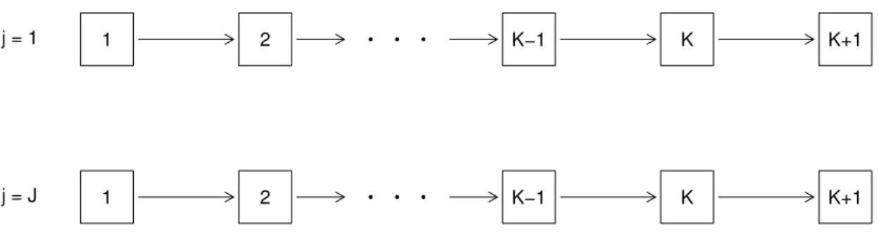
1,2, . . . , K + 1, where state 1 represents no impairment and stateK + 1represents the most severe degree of impairment or damage. In this setting, the only possible transition at any instant in time is to the state representing the next stage of damage (i.e. k → k+ 1 transitions fork = 1,2, . . . , K), thus we use the term “progressive” multistate process.

Consider a disease process in which damage may occur in J organs of affected individuals as illustrated in Figure 1. We restrict attention to a vector ofp×1“cluster-level” covariates,Xj =X,

common to all processes and representing, for example, a genetic marker, sex or treatment. Let Tjk denote the time of a k → k + 1 transition for process j, k = 1, . . . , K, where 0 < Tj1 < Tj2 <· · · < TjK, j = 1, . . . , J;Tj = (Tj1, . . . , TjK)0, andT = (T10, . . . , TJ0)0. Let(T1K, . . . , TJ K)0

denote the vector of absorption times for the J processes, Tj,−K = (Tj1, . . . , Tj,K−1)0 denote the vector of transition times up to and including the penultimate transition time for process j, T−j,k =

(T1k, . . . , Tj−1,k, Tj+1,k, . . . , TJ k)0 denote the vector ofk → k+ 1 transition times for all processes

except processj, andT−j,−K = (T−0j,1, . . . , T 0

−j,K−1)0. We lettjk,tj,t,tj,−K,t−j,k andt−j,−K denote

the corresponding realizations. A fully specified multivariate multistate model requires a complete specification of the joint density of all transition times given the covariateX =x, which we denote byf(t|x). This can be decomposed into a product of conditional and unconditional densities, and one can make working (conditional) independence assumptions to avoid specification of (conditional)

(3)

de-pendencies of secondary interest. These conditional independence assumptions lead to simplifications and motivate our use of composite likelihood; see Section 3. There are many ways to decompose the joint density, and different decompositions and working independence assumptions may prove useful for addressing different research questions.

1 2 K−1 K K+1

j = J j = 1

Figure 1: State space diagram for multivariate multistate processes.

Our first goal is to model each component marginal process in a way that is similar to the way one would for a single multistate process. Specifically, we wish to consider the case in which each com-ponent processjis modeled under a Markov assumption with multiplicative intensities for transitions of statekof the form

λjk(t|x;θjk) = λjk(t;αjk) exp(x0βjk),

whereλjk(t;αjk)is a baseline intensity function indexed by a parameter vector αjk, βjk is a p×1

vector of regression coefficients and θjk = (α0jk, β

0 jk) 0 . If θj = (θj01, . . . , θ 0 jK) 0 , the density ofTj =

(Tj1, . . . , TjK)0givenX =xhas the form

f(tj|x;θj) = K Y k=1 ( λjk(tjk|x;θjk) exp " − Z tjk tj,k−1 λjk(u|x;θjk)du #) , (2.1)

where0 = tj0 < tj1 <· · ·< tjK forj = 1, . . . , J (Andersen et al., 1993).

Our second goal is to parameterize the association between processes which we do in terms of the joint survivor function of the absorption times(T1K, . . . , TJ K)0 conditional onX =xas

P(T1K ≥t1K, . . . , TJ K ≥tJ K|x;ψ) = C(F1K(t1K|x;θ1), . . . ,FJ K(tJ K|x;θJ);φ), (2.2)

(Nelsen, 2006, Patton, 2006), whereC(·;φ)is a multivariate copula function with association parame-tersφ,FjK(tjK|x;θj)is the marginal survivor function of the entry time to the absorption stateK+ 1,

θ = (θ₁0, . . . , θ0_J)0andψ = (θ0, φ0)0. If processjis Markov,FjK(t|x)is obtained as the complement of

the[1, K+1]entry of the transition probability matrix_Pj(0, t|x)of processj, which can be calculated

by product integration (Andersen et al., 1993) via Pj(0, t|x) =

Y

u∈(0,t]

[_I+d_Aj(u|x)] ,

where_Iis an identity matrix of sizeK+ 1,

(4)

andΛjk(t|x) = Rt

0 λjk(u|x)du,k = 1,2, . . . , K.

To ensure our model satisfies these two goals, we decompose the joint density f(t|x;ψ) in a particular way and make “working” conditional independence assumptions about the dependence relations of little interest. First, we decompose the full densityf(t|x;ψ)as

f(t|x;ψ) = f(t1,−K, . . . , tJ,−K|t1K, . . . , tJ K, x;ψ)·f(t1K, . . . , tJ K|x;ψ), (2.3)

which can be rewritten as f(t|x;ψ) =

J Y

j=1

f(tj,−K|t1K, . . . , tJ K, x;ψ)·f(t1K, . . . , tJ K|x;ψ), (2.4)

under the first set of working conditional independence assumptions, A.1 Tj,−K⊥T−j,−K|(T1K, . . . , TJ K, X0)0,

where Y1⊥Y2|Y3 implies fY1,Y2|Y3(y1, y2|y3) = fY1|Y3(y1|y3)fY2|Y3(y2|y3) for random vectors Y1, Y2 andY3. This assumption states that intermediate transition times are independent between processes given covariates and the absorption times for all processes. Expression (2.4) can be further simplified to f(t|x;ψ) = J Y j=1 f(tj,−K|tjK, x;θj)·f(t1K, . . . , tJ K|x;ψ), (2.5)

by invoking the second set of working assumptions applied to the first product term of (2.5) : A.2 Tj,−K⊥T−j,K|(TjK, X0)0.

This assumption states that the intermediate transition times for a particular process are conditionally independent of the absorption times for other processes given its own absorption time. The second item in (2.5) is the joint density of the absorption times, which by the copula formulation in (2.2) has the form f(t1K, . . . , tJ K|x;ψ) = J Y j=1 f(tjK|x;θj)·c(F1K(t1K|x;θ1), . . . ,FJ K(tJ K|x;θJ);φ), (2.6)

wherec(·)is the copula density function of the copulaC(·)in (2.2). By (2.5) and (2.6), the full density f(t|x;ψ)can then be expressed as

f(t|x;ψ) =

J Y

j=1

f(tj|x;θj)·c(F1K(t1K|x;θ1), . . . ,FJ K(tJ K|x;θJ);φ), (2.7)

where the firstJ components are density functions which correspond to marginal models (2.1), and the last component is the copula density function governing the absorption time distribution.

Some conditional dependence structures are left unspecified under the working conditional inde-pendence assumptions A.1 and A.2, so (2.7) only involves a partial specification of the full likelihood (2.3). As such it can be characterized as a composite likelihood for a fully observed joint multistate processes. The working independence approach of Lee and Kim (1998) involving separate marginal analyses can be cast in this framework. They require their multiple multistate model to have the first feature only, and do not model the dependence structure between processes. Thus (2.1) is a composite likelihood under working independence assumptions between processes. We also remark that, in the special caseJ = 2andK = 2, our model can be also justified by a vine copula decomposition (Joe, 1996, Bedford and Cooke, 2001, 2002, Aas and Berg, 2009, Aas et al., 2009).

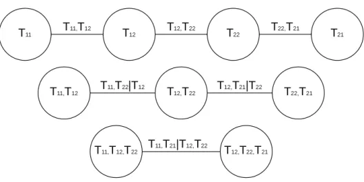
Figure 2 shows the decomposition specification of the joint density f(t|x;ψ)according to a D-vine (Kurowicka and Cooke, 2005). Each edge in Figure 2 corresponds to a pair-copula (conditional)

(5)

Figure 2: A D-vine decomposition with four variables.

density, e.g. the edgeT11, T22|T12 corresponds to the conditional copula density c(F(t11|t12, x;θ1),

F(t22|t12, x;θ, φ);φ2). The joint density ofTj1, Tj2is given by (2.1), which is not induced by a copula function, forj = 1,2. The joint densityf(t|x;ψ)corresponding to the D-vine illustrated in Figure 2 may be written as

· c(F(t11|t12, x;θ1),F(t22|t12, x;θ, φ);φ2)·c(F(t12|t22, x;θ, φ),F(t21|t22, x;θ2);φ3)

· c(F(t11|t12, t22, x;θ, φ, φ2),F(t21|t12, t22, x;θ, φ, φ3);φ4). (2.8) Conditional independence assumptions are commonly used in the vine copula framework to reduce the number of pair copulas in the decomposition and hence simplify model construction. Our working conditional independence assumptions, whenJ =K = 2, have the forms of

(A.1) T11⊥T21|(T12, T22, X0)0,

(A.2) T11⊥T22|(T12, X0)0,T21⊥T12|(T22, X0)0,

the same as vine copula conditional independence assumptions making the last three terms of (2.8) equal to one. Thus (2.8) is simplified to a truncated vine (Brechmann et al., 2012)

The marginal processes are compatible with those of a single multistate process and each compo-nent process in (2.7) yields parameters with a straightforward interpretation in terms of transition rates and covariate effects. However, our model features a parameterized association structure and hence a measure of the association can be readily calculated based on the functional form of the copulaC(·)

and association parameter φ(Genest and MacKay, 1986). In addition, our working assumptions are weaker than those of complete independence, and may lead to more efficient estimation. Under (2.7), one can separately specify the marginal models for each process and the model for the association among the processes, thereby avoiding specification of the conditional dependence structures of little interest. Many options exist for specification of the marginal models and the association models, of course making (2.7) quite flexible.

(6)

3 ESTIMATION AND

INFERENCE

3.1 NOTATION FORINTERVAL-CENSORED DATA

When individuals are assessed intermittently, the times of transitions between states are subject to interval censoring. This is routinely the case when the processes relate to damage of internal or-gans. For notational convenience, we restrict attention to the case in which all processes are assessed at the same M (> 1) time points denoted by v0 < v1 < · · · < vM < vM+1, where v0 = 0, vM+1 = ∞. Let V1, . . . , VM be a sequence of corresponding random variables with joint density

fV1,...,VM(v1, . . . , vM;ν) indexed byν. Let Zj(t)represent the state occupied by the disease process

j at time t and assume that Zj(v0) = 1 with probability 1, j = 1, . . . , J. We next define random variables which record the number of “transitions” of a particular type and letN_jk`m =I(Zj(vm−1) = k, Zj(vm) = `) indicate whether process j occupied state k at assessment time vm−1 and state ` at vm. The data available then consist of the inspection times, the indicators and the covariate

vector:(vm, Njk`m , `=k, . . . , K+ 1, k= 1, . . . , K, j= 1, . . . , J), m= 1, . . . , M, X .The data

can also be expressed as the left and right end point of the censoring intervals:{Tjk ∈(Ljk, Rjk]; k=

1, . . . , K, j = 1, . . . , J, X}, where M(t) = argmax_m{vm < t}, Ljk = vM(Tjk) and Rjk =

vM(Tjk)+1.

3.2 COMPOSITE LIKELIHOODCONSTRUCTION

We assume that the parameterν associated with the inspection process in fV1,...,VM(v1, . . . , vM;ν)is functionally independent of the parameter of interestψ, making the inspection process non-infomative. Under the conditions of Gr¨uger et al. (1991), we proceed to construct the full likelihood arising from intermittent inspection of a joint multistate process as if the inspection times are fixed and hence, in what follows we restrict attention to

L(ψ) =P(Tjk ∈(ljk, rjk]; k = 1, . . . , K; j = 1, . . . , J|x, v1, . . . , vM;ψ). (3.1)

The likelihood in (3.1) is obtained by computingJ ×K -dimensional integrals over the full density f(t|x;ψ)in (2.3). For example, in the special case J = K = 2, 4D integrals involvingf(t|x;ψ)

in (2.8) are required. When J or K are large, the likelihood involves computationally demanding high-dimensional integration. Use of composite likelihood enables some simplification in model specification and increases robustness to model misspecification.

Lee and Kim (1998) discuss the case when interest lies only in estimation of marginal parameters. If a working independence assumption among processes is reasonable, the estimation problem sim-plifies to one that has been addressed in the literature (Kalbfleisch and Lawless, 1985). Since process j is Markov, the composite likelihood of processjis

CL1(θj) = M Y m=1 K Y k=1 K+1 Y `=k P(Zj(vm) = `|Zj(vm−1) = k, x;θj)n m jk` . (3.2)

A Fisher-scoring or Newton-Raphson algorithm can be used for estimation, and robust variance esti-mation is described in Appendix A of supplementary material available atBiostatisticsonline.

If both marginal and association parameters are of interest in the interval-censored setting, we make the following working conditional independence assumptions:

(A.3) Tj,−K⊥T−j,−K|(T1K ∈(L1K, R1K], . . . , TJ K ∈(LJ K, RJ K], X0)0,

(7)

These are slightly different from assumptions A.1 and A.2, but enable one to write down the composite likelihood arising from intermittent inspection:

CL2(ψ) = J Y j=1 P(Tjk ∈(ljk, rjk], k= 1, . . . , K−1|TjK ∈(ljK, rjK], x;θj) × P (TjK ∈(ljK, rjK], j = 1, . . . , J|x;ψ) , (3.3)

in which theJ + 1components are analogous to those in (2.7). In (3.3), P (TjK ∈(ljK, rjK], j = 1, . . . , J;ψ) =

X

a∈A

(−1)daC(F1K(a1K|x;θ1), . . . ,FJ K(aJ K|x;θJ);φ), (3.4)

wherea = (a1K, . . . , aJ K)0, A = {a:ajK ∈ {ljK, rjK}, j = 1, . . . , J}, da = PJ_j₌₁I(ajK = rjK),

and (3.4) involves a summation of2K _{items. Note that since}_{_T

jk ∈ (Ljk, Rjk]; k = 1, . . . , K, j =

1, . . . , J, X}contains the same information as{(vm, Njk`m , ` = k, . . . , K + 1, k = 1, . . . , K, j =

1, . . . , J), m = 1, . . . , M, X},P(Tjk ∈ (ljk, rjk], k = 1, . . . , K;θj)is equal to the marginal

likeli-hoodLj(θj)in (3.2). The composite likelihood (3.3) can therefore be written as

CL2(ψ) = J Y j=1 Lj(θj) FjK(ljK|x;θj)− FjK(rjK|x;θj) ·P (TjK ∈(ljK, rjK], j = 1, . . . , J|x;ψ).(3.5)

A composite likelihood can alternatively be built using the “construction method” (Varin, 2008) by usingJ marginal likelihoods to obtain marginal estimates and using the joint probability of theJ absorption times to estimate the association parameters. The composite likelihood is then

CL3(ψ) =

J Y

j=1

Lj(θj)·P (TjK ∈(ljK, rjK], j = 1, . . . , J|x;ψ) . (3.6)

Composite likelihoods based on (3.2), (3.5) and (3.6) represent simplifications to the full likeli-hood (3.1) and so may lead to some loss of efficiency (see Appendix B of supplementary material available atBiostatisticsonline), but their use introduces robustness (see Appendix C of supplemen-tary material available atBiostatisticsonline) and significant computational advantages. The compos-ite likelihood based on (3.2) is obtained under the strongest working independence assumption and so does not provide estimation of any association parameters and would be expected to be the least efficient. The composite likelihoods in (3.5) and (3.6) are constructed based on different ideas but have similar forms, and both avoid the need for high-dimensional integration.

3.3 TWO-STAGEESTIMATION

A two-stage estimation procedure (Shih and Louis, 1995, Newey and McFadden, 1994, Zhao and Joe, 2005) is possible with the formulation described due to the copula structure of the association model. In the first stage, an estimate of the marginal parameters θj is obtained for each process j

using the marginal likelihood (3.2), j = 1, . . . , J. In the second stage, the estimate θˆis inserted into composite likelihoodCL2(ψ)in (3.5) orCL3(ψ)in (3.6), which is then maximized with respect to φ to obtain an estimate φ. With regard to the two composite likelihoods (3.5) and (3.6), only˜ P (TjK ∈(ljK, rjK], j = 1, . . . , J;ψ)in (3.4) contains the association parameters, and so this is the

objective function in the second stage. Shih and Louis (1995) develop the asymptotic distribution for the case when the association parameter is a scalar. The corresponding asymptotic results for a vector of association parameters are given in Newey and McFadden (1994).

(8)

4 SIMULATION

STUDIES AND

I

LLUSTRATION 4.1 DESIGN AND ANALYSIS OFSIMULATIONSTUDIES

The simulation studies conducted here are designed to assess the finite sample properties of estimators from the various composite likelihoods. We consider two processes with three states each, where state 1 represents a “normal” condition, state 2 represents “abnormal”, and state 3 represents the absorbing state of “organ damage”; we assume that all subjects start from state 1 for both processes. We consider one Bernoulli covariateX, with P(X = 1) = 0.5. We assume here that there areM = 10common inspection times evenly spaced over the interval (0,1], giving visit times vm = 0.1×m for m =

1, . . . ,10. We generate data from the full density of the form (2.8) as illustrated in Appendix D of supplementary material available at Biostatisticsonline, where the marginal model is a progressive time-homogeneous Markov processes with transition intensities λjk(t|x;θjk) = αjkexp(xβjk) for

j, k = 1,2. We assume that the two processes have the same margins, as would be the case with clustered processes, so thatα1k =α2k andβ1k =β2k fork = 1,2. We setβj1 = log(1.25)to reflect a mild increase of the risk of transition from state 1 to 2 when X = 1 and set βj2 = log(1.4) to reflect a moderate effect on increasing the risk of transition from state 2 to 3 in both processes. The baseline transition intensitiesαjkforj, k = 1,2are set under the following constraints: (i) the baseline

transition rate out of state 2 is 1.5 times of that out of state 1, i.e. αj2 = 1.5αj1 forj = 1,2; (ii) the probability of both processes being in state 3 by time 1 is 0.4 in the control group. These constraints giveαj1 = 1.8148andαj2 = 2.7221. For the association model, we consider four scenarios including the following: (i) the four copulas in (2.8) are induced by Clayton copulas when the dependencies are strong; specifically, Kendall’sτ, τ2, τ3 andτ4 are equal to 0.8, 0.7, 0.6 and 0.5, respectively, (ii) Clayton copulas when the dependencies are weak; specifically, Kendall’s τ, τ2, τ3 andτ4 are equal to 0.4, 0.3, 0.2 and 0.1, respectively, (iii) Frank copulas when the dependencies are positive and moderate; specifically, Kendall’sτ, τ2, τ3 andτ4 are equal to 0.6, 0.5, 0.4 and 0.3, respectively, and (iv) Frank copulas when the dependencies are negative and moderate; specifically, Kendall’sτ,τ2,τ3 and τ4 are equal to -0.6, -0.5, -0.4 and -0.3, respectively. (φ, φ2, φ3, φ4)0 = (3,8,2,4.6667)0 giving Kendall’sτ’s of(0.6,0.8,0.5,0.7)0, respectively (Nelsen, 2006). Two thousand samples are simulated ofn = 1000individuals each.

For each dataset, analyses are carried out based on the composite likelihoods (3.5) and (3.6), and two-stage estimation to estimateψ. The empirical biases (BIAS), average standard error (ASE), em-pirical standard error (ESE), and emem-pirical coverage probability (ECP) are evaluated for all parameter estimates and reported in Table 1. The ASE is the average of the 2000 sample standard errors, the ESE is the standard deviation of 2000 parameter estimates, and the ECP is the proportion of all trials for which the composite likelihood Wald-based 95% confidence intervals (CIs) contain respective true parameter value (Molenberghs and Verbeke, 2005).

As expected from the asymptotic theory, the empirical biases are all very small for estimates of the marginal parameters and the association parameters using all methods. The ASE and ESE are consistent with each other and the ECPs are all very close to the nominal confidence level of 95%, suggesting that the methods proposed provide a valid basis for inference. The relative precision of the marginal parameters estimates shows that the two-stage procedure incurs a loss of efficiency, but the estimates of the association parameter by the two-stage procedure are of comparable precision. We also note that estimates of the marginal parameters for transitions from the mild to intermediate state obtained via the composite likelihood (3.5) is slightly more efficient than their counterparts from the composite likelihood (3.6).

(9)

T able 1: Frequenc y properties of estimators of parameters using a composite lik elihood and tw o-stage estimation procedure under a correctly specified model; 1000 observ ations per sample; 2000 simulations. C L 2 in (3.5) C L 3 in (3.6) TS Relati v e ef ficienc y P ara T rue BIAS ASE ESE ECP BIAS ASE ES E ECP BIAS ASE ESE ECP R E 1 R E 2 Strong dependence and Clayton copula 1 log ( α 11 ) 0.623 -0.001 0.045 0.045 0.944 -0.001 0.046 0.047 0.944 -0.001 0.049 0.050 0.944 0.929 0.825 log ( α 12 ) 1.029 -0.001 0.052 0.051 0.956 -0.001 0.053 0.053 0.957 -0.001 0.056 0.055 0.954 0.962 0.886 log ( α 21 ) 0.623 -0.001 0.045 0.044 0.960 -0.001 0.046 0.045 0.959 -0.001 0.049 0.048 0.958 0.943 0.838 log ( α 22 ) 1.029 -0.001 0.052 0.052 0.951 -0.001 0.053 0.054 0.945 -0.001 0.056 0.056 0.944 0.938 0.850 β 11 0.223 -0.001 0.056 0.055 0.954 -0.001 0.060 0.060 0.950 -0.002 0.068 0.068 0.951 0.850 0.654 β 12 0.336 0.002 0.071 0.070 0.954 0.001 0.072 0.071 0.952 0.001 0.075 0.075 0.945 0.961 0.859 β 21 0.223 -0.001 0.056 0.055 0.954 -0.001 0.060 0.059 0.954 -0.001 0.068 0.068 0.948 0.859 0.654 β 22 0.336 0.000 0.070 0.069 0.954 0.000 0.071 0.071 0.949 -0.001 0.075 0.076 0.946 0.939 0.813 log ( φ ) 2.079 0.004 0.053 0.054 0.938 0.003 0.053 0.054 0.938 0.001 0.053 0.054 0.938 0.984 0.992 W eak dependence and Clayton copula 2 log ( α 11 ) 0.561 -0.001 0.048 0.048 0.948 -0.001 0.048 0.049 0.946 -0.001 0.049 0.050 0.946 0.949 0.914 log ( α 12 ) 0.967 -0.002 0.057 0.056 0.956 -0.002 0.057 0.056 0.952 -0.002 0.057 0.055 0.952 0.997 1.000 log ( α 21 ) 0.561 -0.001 0.048 0.048 0.952 -0.001 0.049 0.049 0.952 -0.001 0.049 0.050 0.954 0.964 0.931 log ( α 22 ) 0.967 -0.001 0.057 0.056 0.953 -0.001 0.057 0.057 0.953 -0.001 0.057 0.057 0.952 0.984 0.986 β 11 0.223 -0.002 0.065 0.064 0.951 -0.002 0.066 0.067 0.949 -0.002 0.068 0.069 0.946 0.909 0.844 β 12 0.336 0.002 0.077 0.077 0.950 0.002 0.077 0.077 0.952 0.002 0.077 0.077 0.947 0.997 0.996 β 21 0.223 0.000 0.064 0.066 0.946 0.000 0.066 0.068 0.945 0.000 0.068 0.070 0.941 0.927 0.865 β 22 0.336 0.001 0.077 0.077 0.953 0.001 0.077 0.078 0.948 0.001 0.077 0.078 0.946 0.995 0.993 log ( φ ) 0.288 0.002 0.083 0.085 0.944 0.001 0.082 0.084 0.944 0.000 0.082 0.084 0.943 1.021 1.013 Positi v e dependence and Frank copula 3 log ( α 11 ) 0.588 -0.001 0.049 0.048 0.946 -0.001 0.049 0.049 0.943 -0.001 0.049 0.050 0.944 0.974 0.933 log ( α 12 ) 0.994 -0.002 0.054 0.052 0.956 -0.002 0.055 0.053 0.955 -0.002 0.056 0.055 0.958 0.971 0.910 log ( α 21 ) 0.588 -0.001 0.050 0.048 0.950 -0.001 0.048 0.048 0.948 -0.001 0.049 0.049 0.948 0.977 0.935 log ( α 22 ) 0.994 -0.001 0.054 0.054 0.946 -0.001 0.055 0.055 0.946 0.000 0.056 0.057 0.949 0.960 0.895 β 11 0.223 -0.001 0.069 0.065 0.954 -0.002 0.067 0.067 0.950 -0.002 0.068 0.069 0.948 0.950 0.897 β 12 0.336 0.002 0.074 0.073 0.953 0.002 0.075 0.074 0.953 0.001 0.076 0.076 0.948 0.974 0.916 β 21 0.223 0.000 0.071 0.065 0.950 -0.001 0.067 0.067 0.950 -0.001 0.068 0.069 0.947 0.953 0.895 β 22 0.336 0.001 0.074 0.074 0.950 0.000 0.074 0.075 0.947 0.000 0.076 0.077 0.953 0.964 0.903 log ( φ ) 2.071 0.002 0.041 0.042 0.945 0.002 0.041 0.042 0.944 0.001 0.041 0.042 0.944 1.000 0.999 Ne g ati v e dependence and Frank copula 4 log ( α 11 ) 0.418 -0.001 0.050 0.051 0.940 -0.001 0.050 0.052 0.942 -0.001 0.051 0.052 0.940 0.980 0.967 log ( α 12 ) 0.994 -0.002 0.823 0.059 0.960 -0.002 0.061 0.059 0.958 -0.002 0.061 0.059 0.958 1.002 1.002 log ( α 21 ) 0.588 0.002 0.418 0.050 0.948 0.002 0.051 0.051 0.946 0.002 0.051 0.051 0.945 0.981 0.965 log ( α 22 ) 0.994 -0.001 0.823 0.060 0.954 -0.002 0.061 0.060 0.954 -0.002 0.061 0.060 0.956 0.995 0.981 β 11 0.223 -0.002 0.068 0.070 0.946 -0.002 0.069 0.071 0.946 -0.002 0.070 0.072 0.948 0.966 0.946 β 12 0.336 0.002 0.081 0.081 0.947 0.002 0.081 0.081 0.950 0.002 0.082 0.082 0.945 0.997 0.989 β 21 0.223 0.001 0.068 0.069 0.948 0.001 0.070 0.070 0.951 0.001 0.070 0.071 0.950 0.974 0.945 β 22 0.336 0.004 0.081 0.080 0.952 0.004 0.081 0.081 0.948 0.004 0.081 0.081 0.954 0.984 0.972 log ( − φ ) 1.426 0.001 0.060 0.061 0.952 0.001 0.060 0.061 0.952 0.000 0.060 0.061 0.950 1.000 1.000 R E1 is the relati v e ef ficienc y from composite lik elihood (3.6) vs. composite lik elihood (3.5) based on ASE; R E2 is the relati v e ef ficienc y from tw o-stage estimation vs. composite lik elihood (3.5) based on ASE; 1τ 1 =0.8, τ2 =0.7, τ3 =0.6, τ4 =0.5; the copulas in (2.8) are induced by Clayton copulas; 2τ 1 =0.4, τ2 =0.3, τ3 =0.2, τ4 =0.1; the copulas in (2.8) are induced by Clayton copulas; 3τ 1 =0.6, τ2 =0.5, τ3 =0.4, τ4 =0.3; the copulas in (2.8) are induced by Frank copulas; 4τ 1 =-0.6, τ2 =-0.5, τ3 =-0.4, τ4 =-0.3; the copulas in (2.8) are induced by Frank copulas.

(10)

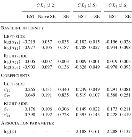
Table 2: Joint analysis of progression in the left and right SI joints in PsA with the covariate HLA B27 and allowing different parameters in the two processes

CL1(3.2) CL2(3.5) CL3(3.6) EST Naive SE SE EST SE EST SE BASELINE INTENSITY LEFT-SIDE log(α11) -0.215 0.057 0.035 -0.182 0.015 -0.196 0.028 log(α12) -0.977 0.105 0.187 -0.788 0.027 -0.944 0.098 RIGHT-SIDE log(α21) -0.005 0.007 0.003 0.009 0.001 0.019 0.003 log(α22) -0.903 0.097 0.136 -0.828 0.049 -0.978 0.093 COEFFICIENTS LEFT-SIDE β11 0.265 0.131 0.440 0.249 0.049 0.291 0.081 β12 0.649 0.191 0.835 0.519 0.107 0.568 0.251 RIGHT-SIDE β21 0.176 0.106 0.306 0.149 0.022 0.173 0.211 β22 0.398 0.192 0.728 0.395 0.143 0.428 0.419 ASSOCIATION PARAMETER log(φ) - - - 2.188 0.161 2.288 0.137

The marginal estimates using composite likelihood (3.2) are plugged into the composite likelihood (3.5) or (3.6) to obtain

log( ˆφ) = 2.239(SE= 0.246).

4.2 ANALYSIS OFPROGRESSION INJOINT DAMAGE AMONGINDIVIDUALS WITHARTHRITIS We consider data from the University of Toronto Psoriatic Arthritis (PsA) Clinic which are com-prised of several hundred patients enrolled since 1978. We focus on the state of damage of the left and right sacroiliac (SI) joints since damage in these joints signifies the onset of a condition called spondyloarthritis which is associated with considerable disability. The modified Steinbrocker scale (Steinbrocker et al., 1949, Rahman et al., 1998) is a five-point scale used to record the extent of dam-age based on radiographic examination. The states are numbered 1−5 with labels 1 = normal;

2 = equivocal; 3 = abnormal with erosions or sclerosis; 4 = unequivocally abnormal, moderate or advanced sacroilitis showing one or more of erosions, sclerosis, widening, narrowing or partial ankylosis;5 =total ankylosis. In our analysis, we combine states 2 and 3 to form a state representing mild joint damage, and states 4 and 5 as a state denoting moderate to severe damage. We consider the Human Leukocyte Antigen (HLA) B27 as a covariate X, since it is an inherited genetic marker associated with a number of related rheumatic diseases including ankylosing spondylosis. We restrict attention to data as of December 1, 2007, for 640 patients with complete covariate information (HLA B27) and use data obtained at all assessments that the modified Steinbrocker score could be assessed. We allow the covariate HLA B27 to have different effects for the left and right SI joints, and also allow different baseline transition rates for both transition into the mild state and that into moderate-severe state.

The results are summarized in Table 2. The upper part of the table gives estimates (ESTs) and standard errors (SEs) pertaining to baseline transition rates, the middle part is of the regression coef-ficients, and the lower part is for the association parameter. Based on analysis using the composite

(11)

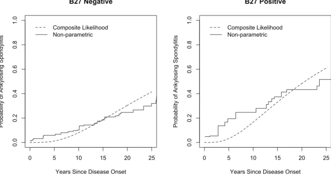
likelihood (3.5), for example, individuals HLA B27 positive have a significantly higher transition rate to mild damage on the left SI joint (relative risk (RR) = 1.28, 95% CI: 1.16–1.41, p < 0.001) and a significantly higher rate of progression to the state of moderate-severe damage on that side (RR = 1.68, 95% CI: 1.33–2.03, p < 0.001). On the right SI joint, being B27 positive is associ-ated with an increased risk of mild damage (RR = 1.16, 95% CI: 1.11–1.21, p < 0.001) and there was evidence of a more rapid onset of moderate-severe damage (RR = 1.48, 95% CI: 1.07–1.90, p <0.001). The estimate of Kendall’sτ based on (3.5) wasτˆ= 0.82(95% CI: 0.77–0.87,p < 0.001) corresponding to significant evidence of a very strong association in progression times to moderate-severe damage. One of the New York criteria (Moll and Wright, 1973) for diagnosis of ankylosing spondylitis is satisfied if(Z1(t), Z2(t)) = (3,3). The joint model is particularly appealing here then, since it permits prediction of time to the development of ankylosing spondylitis. Figure 3 gives plots

0 . 0 0 . 2 0 . 4 0 . 6 0 . 8 1 . 0 B27 Negative

Years Since Disease Onset

Pro b a b ility o f A n kylo sin g Sp o n d ylitis Composite Likelihood Non-parametric 0 5 10 15 20 25 0 . 0 0 . 2 0 . 4 0 . 6 0 . 8 1 . 0 B27 Positive

Pro b a b ility o f A n kylo sin g Sp o n d ylitis Composite Likelihood Non-parametric 0 5 10 15 20 25

Figure 3: Plots of the cumulative probability of ankylosing spondylitis by B27 status according to the composite likelihood (3.5) analysis from the joint model and based on non-parametric estimate of Gentleman and Vandal (2002); for the fitted parametric model the estimated joint probability is P(Z1(t) =Z2(t) = 3|Z1(0) =Z2(0) = 1; ˆψ).

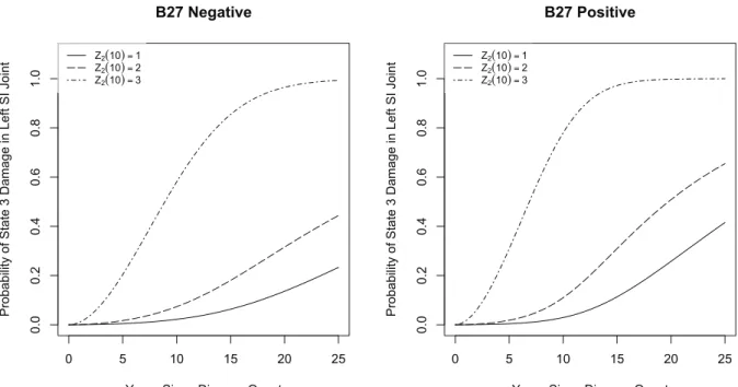
of the cumulative probability of ankylosing spondylitis by this criteria based on the fitted model using the composite likelihood (3.5) as an illustration. The left-hand panel shows this probability estimated for individuals who are B27 negative and the right-hand panel is for B27 positive. Overlaid on these plots are estimates obtained by the graph-theoretic approach to non-parametric estimation of bivariate failure time distribustions with interval-censored data developed in Gentleman and Vandal (2002) and implemented in theR packageMLEcens (Maathuis, 2010); there is reasonable agreement between the estimates. The joint model is also useful for examining how risks of damage in a particular SI joint depend on the damage state of the contralateral SI joint. For example if we consider the risk of the left SI joint exhibiting moderate or severe damage since onset, we can consider three scenarios: the right SI joint developed i) no damage by 10 years, ii) mild damage by 10 years, and iii) moderate-severe damage by 10 years. The fitted model yields estimates asP(Z1(t) = 3|Z1(0) = 1, Z2(10) = 1, x; ˆψ), P(Z1(t) = 3|Z1(0) = 1, Z2(10) = 2, x; ˆψ), andP(Z1(t) = 3|Z1(0) = 1, Z2(10) = 3, x; ˆψ) respec-tively. These are plotted in Figure 4 and reveal that the appreciable estimate of Kendall’sτ leads to a

(12)

strong influence on the conditional probabilities and hence prediction in the course of disease. 0 . 0 0 . 2 0 . 4 0 . 6 0 . 8 1 . 0 B27 Negative

Pro b a b ility o f Sta te 3 Da ma g e in L e ft SI Jo in t Z2(10)= 1 Z2(10)= 2 Z2(10)=3 0 5 10 15 20 25 0 . 0 0 . 2 0 . 4 0 . 6 0 . 8 1 . 0 B27 Positive

Pro b a b ility o f Sta te 3 Da ma g e in L e ft SI Jo in t Z2(10)= 1 Z2(10)= 2 Z2(10)=3 0 5 10 15 20 25

Figure 4: Plots of the estimated conditional probability P(Z1(t) = 3|Z1(0) = 1, Z2(10) = 1, x; ˆψ), P(Z1(t) = 3|Z1(0) = 1, Z2(10) = 2, x; ˆψ)andP(Z1(t) = 3|Z1(0) = 1, Z2(10) = 3, x; ˆψ)according to the composite likelihood (3.5) analysis from the joint model vs. time since disease onset (years).

5 DISCUSSION

In settings where processes are clustered, one may wish to constrain αjk = αk andβjk = βk, j =

1,2, . . . , J, and letα = (α1, . . . , αK)0, β = (β1, . . . , βK)0 and θ = (α0, β0)0 (Lee et al., 1992). We

have restricted attention to the case in which all the process were inspected at the same time. In studies of organ damage in diabetic patients, interest may lie in the processes of diabetic retinopathy and nephropathy (Cook and Lawless, 2013). The extent of damage in the eyes, assessed by a detailed clinical examination, and kidneys, assessed by blood tests or imaging, would routinely be measured at different times. Adaptation of the proposed methods are relatively straightforward to handle this case by allowing processj to be assessed atMj time pointsvj0 < vj1 <· · ·< vj,Mj < vj,Mj+1where vj0 =v0 = 0,vj,Mj+1 =vMj+1 =∞forj = 1, . . . , J.

With interval-censored data arising from intermittent inspection, the composite likelihood ap-proaches and the two-stage methods have computational advantages. These methods also bring about increased robustness but also a certain loss in efficiency. The robustness regarding consistency is sim-ilar in spirit to the robustness of generalized estimating equations (GEE) since both methods avoid specification of the higher-order dependencies (Xu and Reid, 2011). The computational advantages are based on the fact that the composite likelihood is integration-free and is easier to maximize (Varin et al., 2011). As is often the case, the computational convenience and robustness are gained by sac-rificing statistical efficiency, so that the trade-off between those factors needs to taken into account when formulating a composite likelihood function.

The marginal processes may correspond to more general, non-Markov, intensity-based models. Multiple ways of devising estimation strategies in this paper point to the flexibility of estimation.

(13)

We have focused on parametric estimation, but weakly parametric piecewise constant transition rates, GEE, or even more robust semiparametric analysis should be explored for estimation of marginal pa-rameters. Several extensions are possible to the association model. First, we assumed the dependence between the absorption transition time are the same whetherX = 1andX = 0; see (2.2). One could allow different association parameters for different covariate values; indeed entirely different copula functions could be adopted. Secondly, we model the association between absorption times via a cop-ula, but one could set,ujk = exp[−

Rtjk

tj,k−1λjk(s|x;θjk)ds], j = 1, . . . , J, and use a copula function to model associations betweenujk anduj0_k, and hence between the transition timesT_jk andT_j0_k. If a semi-Markov model is adopted for the marginal processes, the association between sojourn times is then modeled, as is routinely done in survival analysis. This is an area of current research.

SUPPLEMENTARY

MATERIAL

Supplementary Material is available at http://biostatistics.oxfordjournals.org.

A

CKNOWLEDGEMENTS

Richard Cook is a Canada Research Chair in Statistical Methods for Health Research. The authors thank Drs Dafna Gladman and Vinod Chandran for helpful discussion regarding the research at the Centre for Prognosis Studies in Rheumatic Disease at the University of Toronto. Conflict of Interest: None declased.

FUNDING

This research was supported by grants from the Natural Sciences and Engineering Research Council of Canada (RGPIN 155849) and the Canadian Institutes for Health Research (FRN 13887).

REFERENCES

Aalen, O. O., Borgan, O., and Gjessing, H. K. (2008). Survival and Event History Analysis: A Point Process Point of View. Springer, New York.

Aas, K. and Berg, D. (2009). Models for construction of multivariate dependence - a comparison study. The European Journal of Finance, 15:639–659.

Aas, K., Czado, C., Frigessi, A., and Bakken, H. (2009). Pair-copula constructions of multiple de-pendence. Insurance: Mathematics and Economics, 44:182–198.

Andersen, P. K., Borgan, O., Gill, R. D., and Keiding, N. (1993). Statistical Models Based on Count-ing Processes. SprCount-inger-Verlag, New York.

Bedford, T. and Cooke, R. M. (2001). Probability density decomposition for conditionally dependent random variables modeled by vines. Annals of Mathematics and Artificial Intelligence, 32:245– 268.

Bedford, T. and Cooke, R. M. (2002). Vines - a new graphical model for dependent random variables. Annals of Statistics, 30:1031–1068.

Besag, J. (1974). Spatial interaction and the statistical analysis of lattice systems. Journal of the Royal Statistical Society - Series B, 36:192–236.

(14)

Brechmann, E. C., Czado, C., and Aas, K. (2012). Truncated regular vines in high dimensions with applications to financial data. Canadian Journal of Statistics, 40.1:68–85.

Cook, R. J. and Lawless, J. F. (2007). The Statistical Analysis of Recurrent Events. Springer, New York.

Cook, R. J. and Lawless, J. F. (2013). Concepts and tests for trend in recurrent event processes. Iranian Journal of Statistics, 12:35–69.

Cook, R. J., Yi, G. Y., Lee, K.-A., and Gladman, D. D. (2004). A conditional Markov model for clustered progressive multistate processes under incomplete observation. Biometrics, 60:436–443. Cox, D. R. and Reid, N. (2004). A note on pseudolikelihood constructed from marginal densities.

Biometrika, 91:729–737.

Genest, C. and MacKay, J. (1986). The joy of copulas: bivariate distributions with uniform marginals. The American Statistician, 40:280–283.

Gentleman, R. C. and Vandal, A. C. (2002). Nonparametric estimation of the bivariate cdf for arbi-trarily censored data. Canadian Journal of Statistics, 30:557–571.

Gr¨uger, J., Kay, R., and Schumacher, M. (1991). The validity of inferences based on incomplete observations in disease state models. Biometrics, 47:595–605.

Hougaard, P. (1999). Multi-state models: a review. Lifetime Data Analysis, 5:239–264. Hougaard, P. (2000). Analysis of Multivariate Survival Data. Springer, New York.

Joe, H. (1996). Families of m-variate distributions with given margins and m(m −1)/2 bivariate dependence parameters. IMS Lecture Notes - Monograph Series, 28:120–141.

Joe, H. (1997). Multivariate Dependence Concepts. Chapman and Hall, London.

Kalbfleisch, J. D. and Lawless, J. F. (1985). The analysis of panel data under a Markov assumption. Journal of the American Statistical Association, 80:863–871.

Kalbfleisch, J. D. and Prentice, R. L. (2002). The Statistical Analysis of Failure Time Data. John Wiley and Sons, New York, 2nd edition.

Kurowicka, D. and Cooke, R. M. (2005). Distribution-free continuous bayesian belief nets. In Wilson, A., Limnios, N., Keller-McNulty, S., and Armijo, Y., editors,Modern Statistical and Mathematical Methods in Reliability. World Scientific Publishing Co. Pte. Ltd., Singapore.

Lawless, J. F. (2003). Statistical Models and Methods for Lifetime Data. Wiley, Hoboken, NJ, 2nd edition.

Lee, E. W. and Kim, M. Y. (1998). The analysis of correlated panel data using a continuous-time Markov model. Biometrics, 54:1638–1644.

Lee, E. W., Wei, L. J., and Amato, D. A. (1992). Cox-type regression analysis for large numbers of small groups of correlated failure time observations. In Klein, J. P. and Goel, P. K., editors,Survival Analysis: State of the Art, pages 237–247. Kluwer Academic Publishers, Dordrecht.

(15)

Lindsay, B. G., Yi, G. Y., and Sun, J. (2011). Issues and strategies in the selection of composite likelihoods. Statistica Sinica, 21:71–105.

Maathuis, M. (2010). MLEcens: Computation of the MLE for bivariate (interval) censored data. http://CRAN.R-project.org/package=MLEcens//R package version 0.1-3.

Molenberghs, G. and Verbeke, G. (2005). Models for Discrete Longitudinal Data. Springer, New York.

Moll, J. M. H. and Wright, V. (1973). New york clinical criteria for ankylosing spondylitis. a statistical evaluation. Annual of Rheumatic Diseases, 32:354–363.

Nelsen, R. B. (2006). An Introduction to Copulas. Springer, New York.

Newey, W. K. and McFadden, D. (1994).Large Sample Estimation and Hypothesis Testing. Handbook of Econometrics, North-Holland.

Patton, A. J. (2006). Modeling asymmetric exchange rate dependence. International Economic Re-view, 47:527–556.

Rahman, P., Gladman, D. D., Cook, R. J., Zhou, Y., Young, G., and Salonen, D. (1998). Radiological assessment in psoriatic arthritis. British Journal of Rheumatology, 37:760–765.

Ross, S. M. (1996). Stochastic Processes. Wiley, New York, 2nd edition.

Satten, G. A. (1999). Estimating the extent of tracking in interval-censored chain-of-events data. Biometrics, 55:1228–1231.

Shih, J. H. and Louis, T. A. (1995). Inferences on the association parameters in copula models for bivariate survival data. Biometrics, 51:1384–1399.

Steinbrocker, O., Traeger, C. H., and Batterman, R. C. (1949). Therapeutic criteria in rheumatoid arthritis. Journal of the American Medical Association, 140:659–662.

Sutradhar, R. and Cook, R. J. (2008). Analysis of interval-censored data from clustered multi-state processes: Application to joint damage in psoriatic arthritis.Journal of the Royal Statistical Society - Series C, 57:553–566.

Therneau, T. M. and Grambsch, P. M. (2000). Modeling Survival Data: Extending the Cox Model. Springer, New York.

Varin, C. (2008). On composite marginal likelihoods. Advances in Statistical Analysis, 92:1–28. Varin, C., Reid, N., and Firth, D. (2011). An overview of composite likelihood methods. Statistics

Sinica, 21:5–42.

Xu, X. and Reid, N. (2011). On the robustness of maximum composite likelihood estimates. Journal of Statistical Planning and Inferences, 141:3047–3054.

Zhao, Y. and Joe, H. (2005). Composite likelihood estimation in multivariate data analysis. The Canadian Journal of Statistics, 33:335–356.

(16)

Web-based Supplementary Materials to

Composite Likelihood for Joint Analysis of Multiple Multistate

Processes via Copulas

LIQUN DIAO

Department of Biostatistics and Computational Biology

,

University of Rochester Medical Center, Rochester, NY, 14642, United States Liqun [email protected]

RICHARD J. COOK

Department of Statistics and Actuarial Science

,

University of Waterloo, Waterloo, ON, N2L 3G1, Canada

W

EB

A

PPENDIX

A: R

EVIEW OF

C

OMPOSITE

L

IKELIHOOD

Composite likelihoods are based on partial specification of the full likelihood (Besag, 1974, Lindsay, 1988, Cox and Reid, 2004, Lindsay et al., 2011). Let{A1, . . . ,AQ}denote a set ofQuser-selected

marginal or conditional events. If a component likelihood Lq(ψ) ∝ f(t ∈ Aq;ψ) is indexed by a

parameterψ, a composite likelihood is simply a product of the component likelihoods,

CL(ψ) = Q Y

q=1

Lq(ψ). (A.1)

When the selected events are not independent, a “working independence assumption” can be invoked and the component likelihoods can simply be multiplied together as in (A.1).

Since each component likelihood is a true likelihood in some context, it has some of the features of an ordinary likelihood; see Lindsay (1988) and Molenberghs and Verbeke (2005) for the asymptotic theory. Under mild regularity conditions, the component score functions satisfyE(∂logLq(ψ)/∂ψ) = 0, and it is apparent from (A.1) that the composite score∂logCL(ψ)/∂ψ is simply the summation of the component score functions; under regularity conditions,E(∂logCL(ψ)/∂ψ) = 0. IfCLi(ψ)

is the composite likelihood contribution from individualiin a sample of nindependent individuals, the overall composite likelihood isQn_i₌₁CLi(ψ)and a consistent estimatorψˆis obtained by solving

Pn i=1∂logCLi(ψ)/∂ψ = 0. Moreover, √ n( ˆψ−ψ)→D N(0,D−1(ψ)B(ψ)D−1(ψ)), asn → ∞, (A.2) where D(ψ) = E −∂ 2_log_CL(ψ) ∂ψ∂ψ0 , (A.3) B(ψ) = E ∂logCL(ψ) ∂ψ ∂logCL(ψ) ∂ψ0 . (A.4)

(17)

In the analysis of a particular dataset, standard errors are estimated based on this result by replacing the expectations in (A.2) with their empirical counterparts and evaluating at the estimateψˆ.

A natural question is how to select{A1, . . . ,AQ}to construct the composite likelihood. One

ap-proach is to construct the composite likelihood from low-dimensional marginal or conditional densi-ties; this is called the “construction method”. Alternatively, a composite likelihood can be constructed by omitting particular terms for a full likelihood; this is referred to as the “omission method” (Varin, 2008). The general guideline for both the construction and the omission method is that the parts kept in the composite likelihood should be informative, easily computed and contain parameters of interest; in contrast, the parts omitted are usually hard to evaluate, not very informative, or pose a significant computational burden. Both approaches invoke a series of working independence assumptions under which we can write down a new, more convenient composite likelihood.

W

EB

A

PPENDIX

B: E

FFICIENCY

L

OSSES

U

NDER

C

OMPOSITE

L

IKELIHOOD Here we report on computations carried out to investigate the efficiency of composite likelihood versus full likelihood analysis in finite samples. We consider the setting with two processes and three states in each as in Section 4.1, but we assume no covariates. We consider two scenarios in which all four copulas in

· c(F(t11|t12, x;θ1),F(t22|t12, x;θ, φ);φ2)·c(F(t12|t22, x;θ, φ),F(t21|t22, x;θ2);φ3)

· c(F(t11|t12, t22, x;θ, φ, φ2),F(t21|t12, t22, x;θ, φ, φ3);φ4) (B.1)

are Clayton copulas and in which they are Frank copulas. The values for Kendall’s τ in the four copulas in (B.1) are assumed to be proportional to one another such that

τ4 = 0.8τ3 = 0.82τ2 = 0.83τ .

We evaluate the efficiency loss versus maximum likelihood in estimation of the marginal pa-rameters α = (α11, α12, α21, α22)0 under composite likelihood methods (3.2), (3.5) and (3.6). The

efficiency of the estimators of the vector of transition ratesα using composite likelihood CL(α) is defined as

Eff.(α) = diag(G

−1_(α))

diag(_D−1_(α)

B(α)D−1(α)) ,

where _G(α) = E[−∂2_log_{L(α)/∂α∂α}0_] _{is the Fisher information of the full likelihood, and}

D(α)

and_B(α)are given in (A.3) and (A.4) respectively. We approximate the Fisher information_G(α)by computing b G(α) =− 1 n n X i=1 ∂2_log_L i(α) ∂α∂α0 .

using Monte Carlo methods. Moreover we let_D(α)and_B(α)be likewise approximated by

b D(α) = − 1 n n X i=1 ∂2_log_CL i(α) ∂α∂α0 , and b B(α) = 1 n n X i=1 ∂logCLi(α) ∂α ∂logCLi(α) ∂α0

(18)

respectively. The efficiency Eff.(α)can be approximated by diagGb−1(α)

diagDb−1(α)bB(α)bD−1(α)

. (B.2)

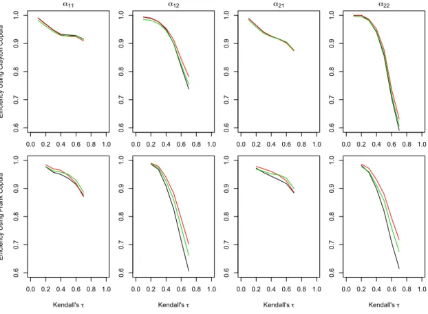
The results are illustrated in Figure 1. The plots in the first row arise from the model involving Clayton copulas and the plots in the second row arise from Frank copulas. In each of the eight plots, the y-axis represents the efficiency given by the corresponding element of (B.2) and the x -axis represents the value of Kendall’s τ. The black line corresponds to estimates using composite likelihood (3.2), the red line corresponds to the estimates base on composite likelihood (3.5), and the green line corresponds to those based on composite likelihood (3.6). As would be expected, the loss of efficiency increases as the dependence between processes increases. It is also apparent that the estimates based on composite likelihood (3.5) are the most efficient and those based on composite likelihood (3.2) are the least efficient in the most scenarios. Under the Frank copula one can consider negative values of Kendall’sτ in which case it becomes apparent that the efficiency curves, while not symmetric, display the similar trend in that the loss of efficiency becomes more appreciable as the negative dependence gets stronger.

W

EB

A

PPENDIX

C: R

OBUSTNESS OF

C

OMPOSITE

L

IKELIHOOD

E

STIMATORS To provide insight into robustness regarding consistency of composite likelihood, we conducted sim-ulation studies involving misspecified copula models in the full density (B.1) and examined the per-formance of estimates of the parameters (θ0, φ)0 based on composite likelihood. We followed the simulation design and the configuration of the marginal parameters given in Section 4.1. For the as-sociation model we considered scenarios in which either the copula governing the absorption times and indexed byφwas misspecified as a Frank copula, or the three conditional copulas indexed byφ2, φ3 andφ4 in (B.1), were Frank copulas; in all cases analyses were conducted based on four Clayton

copulas. We considered strong dependence between processes by setting Kendall’sτ = 0.8,τ2 = 0.7,

τ3 = 0.6andτ4 = 0.5, and weak dependence between with processes by setting Kendall’sτ = 0.4,

τ2 = 0.3, τ3 = 0.2andτ4 = 0.1. We consider a sample size of 1000 individuals per simulation and

2000 simulations.

The results are reported in Table 1. The two upper panels reveal that when the copula governing the absorption times is misspecified, empirical biases are quite appreciable for both the association parameterφgoverning the association between the absorption times, and the marginal parametersθ; the biases are larger when the dependencies are stronger. The two panels on the bottom display the biases when the three conditional copulas are misspecified; these are negligible for both the marginal parametersθand the association parameterφwhether the dependencies between processes are large or small. We also observe close agreement between the average asymptotic standard errors (ASE) and empirical standard errors (ESE) and between empirical coverage probability (ECP) and 95% nominal level. In the other words, the estimates for(θ0, φ)0based on the composite likelihood methods and the two-stage estimation method are valid even with misspecified conditional copulas in the full density (B.1), which demonstrates robustness of composite likelihood to some degree of model misspecifi-cation. The composite likelihood methods only require correct specification of the joint density of absorption times to produce valid estimates, which is weaker than full likelihood requiring correct specification of the full density.

We remark in addition that the choice of the copula governing the absorption times becomes an important issue and it can be approached by using model selection techniques in the context of com-posite likelihood. Varin and Vidoni (2005) proposed comcom-posite Akaike Information Criteria (AIC)

(19)

and Gao and Song (2011) proposed composite Bayesian Information Criteria (BIC), which are ana-logues of AIC and BIC for model selection derived in the framework of composite likelihood.

In the current setting it is also possible to carry out model fitting in stages. Given the copula formulation, separate fits to the marginal processes are possible and diagnostics can be carried out using standard methods (Lawless, 2003) for survival analysis (i.e. based on hazard-based residuals, linearization plots, etc.). Assessing validity of assumptions about the dependence structure is more challenging but again strategies can be borrowed from the survival analysis literature. Work by Genest et al. (2006, 2009) involves use of the probability integral transform of the copula model and is proposed in the context of nonparametric estimates of the marginal distributions for time to event data. This idea can be borrowed and applied to parametric models but inferences about the copula would be predicated on correct specification of the marginal absorption time distributions in our setting. Residual forms of dependence can also be investigated by generalizing the intensity-based models of the marginal processes and testing the need for this type of model expansion.

W

EB

A

PPENDIX

D: D

ATA

S

IMULATION

P

ROCEDURE IN

N

UMERICAL

S

TUDIES Data simulation is conducted by R. The data are generated from the full density (B.1), where the marginal processes are progressive time-homogeneous Markov processes with transition intensities

λjk(t|x;θjk) = αjkexp(xβjk)forj, k = 1,2.

The data generation procedure involves the following steps:

1. SimulateT11givenX =xwhose survival function isF11(t11|x;θ11) = exp(−α11exβ11t11).

2. SimulateT12givenT11 =t11, X =xfromF(t12|t11, x;θ12) = exp[−α12exβ12(t12−t11)].

3. SimulateT22givenT11 =t11, T12 =t12, X =xfrom

F(t22|t12, t11, x;θ, φ, φ2) = ∂C(u1, u2;φ2) ∂u2 u1=F(t22|t12,x;θ,φ),u2=F(t11|t12,x;θ1) where F(t22|t12, x;θ, φ) = ∂C(u1, u2;φ) ∂u2 u1=F22(t22|x;θ2),u2=F12(t12|x;θ1) F(t11|t12, x;θ1) = exp[(α12exβ12 −α11exβ11)t11]−exp[(α12exβ12 −α11exβ11)t12] 1−exp[(α12exβ12 −α11exβ11)t12] Fj2(tj2|x;θj) = αj2exβj2 αj2exβj2 −αj1exβj1 exp(−αj1exβj1tj2)− αj1exβj1 αj2exβj2 −αj1exβj1 exp(−αj2exβj2tj2) forj = 1,2.

4. SimulateT21givenT11 =t11, T12 =t12, T22 =t22, X =xfrom

(20)

R

EFERENCES

Besag, J. (1974). Spatial interaction and the statistical analysis of lattice systems. Journal of the Royal Statistical Society - Series B, 36:192–236.

Cox, D. R. and Reid, N. (2004). A note on pseudolikelihood constructed from marginal densities.

Biometrika, 91:729–737.

Gao, X. and Song, P. X.-K. (2011). Composite likelihood EM algorithm with applications to multi-variate hidden Markov model. Statistica Sinica, 21:165–185.

Genest, C., Quessy, J. F., and R´emillard, B. (2006). Goodness-of-fit procedures for copula models based on the probability integral transformation.Scandinavian Journal of Statistics, 33.2:337–366. Genest, C., R´emillard, B., and Beaudoin, D. (2009). Goodness-of-fit tests for copulas: A review and

a power study. Insurance: Mathematics and Economics, 44.2:199–213.

Lawless, J. F. (2003). Statistical Models and Methods for Lifetime Data. Wiley, Hoboken, NJ, 2nd edition.

Lindsay, B. G. (1988). Composite likelihood methods. Contemporary Mathematics, 80:221–239. Lindsay, B. G., Yi, G. Y., and Sun, J. (2011). Issues and strategies in the selection of composite

likelihoods. Statistica Sinica, 21:71–105.

Molenberghs, G. and Verbeke, G. (2005). Models for Discrete Longitudinal Data. Springer, New York.

Varin, C. (2008). On composite marginal likelihoods. Advances in Statistical Analysis, 92:1–28. Varin, C. and Vidoni, P. (2005). A note on composite likelihood inference and model selection.

(21)

0.0 0.2 0.4 0.6 0.8 1.0 0.6 0.7 0.8 0.9 1.0 α11 Ef fici en cy U si ng C la yt on C op ul a 0.0 0.2 0.4 0.6 0.8 1.0 0.6 0.7 0.8 0.9 1.0 α12 0.0 0.2 0.4 0.6 0.8 1.0 0.6 0.7 0.8 0.9 1.0 α21 0.0 0.2 0.4 0.6 0.8 1.0 0.6 0.7 0.8 0.9 1.0 α22 0.0 0.2 0.4 0.6 0.8 1.0 0.6 0.7 0.8 0.9 1.0 Kendall's τ Ef fici en cy U si ng F ra nk C op ul a 0.0 0.2 0.4 0.6 0.8 1.0 0.6 0.7 0.8 0.9 1.0 Kendall's τ 0.0 0.2 0.4 0.6 0.8 1.0 0.6 0.7 0.8 0.9 1.0 Kendall's τ 0.0 0.2 0.4 0.6 0.8 1.0 0.6 0.7 0.8 0.9 1.0 Kendall's τ

Figure 1: Plots of efficiency as a function of Kendall’sτfor Clayton and Frank copulas with the black line corresponding to composite likelihood (3.2), the red line composite likelihood (3.5) and the green line composite likelihood (3.6)

(22)

Table 1: Frequency properties of estimators of parameters using composite likelihood and two-stage estimation procedure under misspecified model; 1000 observations per sample; 2000 simulations.

CL2in (3.5) CL3in (3.6) Two-Stage Rel. Eff. Para True BIAS ASE ESE ECP BIAS ASE ESE ECP BIAS ASE ESE ECP RE1 RE2

Strong Dependence and Copula Governing Absorption Times Misspecified1

log(α11) 0.617 0.053 0.045 0.046 0.782 0.021 0.047 0.047 0.917 -0.001 0.049 0.050 0.946 0.939 0.848 log(α12) 1.023 0.058 0.051 0.050 0.808 0.026 0.053 0.052 0.919 -0.001 0.056 0.055 0.955 0.921 0.831 log(α21) 0.617 0.052 0.046 0.045 0.794 0.021 0.047 0.046 0.928 -0.001 0.049 0.048 0.956 0.950 0.857 log(α22) 1.023 0.059 0.051 0.050 0.786 0.027 0.053 0.053 0.922 0.000 0.056 0.056 0.945 0.908 0.809 β11 0.223 -0.071 0.059 0.059 0.779 -0.040 0.062 0.062 0.902 -0.002 0.068 0.069 0.950 0.898 0.739 β12 0.336 -0.047 0.072 0.071 0.900 -0.015 0.073 0.072 0.946 0.002 0.076 0.075 0.945 0.951 0.876 β21 0.223 -0.070 0.060 0.059 0.786 -0.039 0.063 0.062 0.904 -0.001 0.068 0.068 0.950 0.907 0.753 β22 0.336 -0.049 0.071 0.071 0.890 -0.017 0.073 0.073 0.942 -0.001 0.076 0.077 0.947 0.939 0.845 log(φ) 2.901 -0.781 0.054 0.055 0.000 -0.764 0.053 0.054 0.000 -0.757 0.053 0.057 0.000 1.033 0.940 Weak Dependence and Copula Governing Absorption Times Misspecified2

log(α11) 0.557 0.020 0.048 0.048 0.922 0.008 0.049 0.049 0.939 -0.001 0.049 0.050 0.944 0.951 0.920 log(α12) 0.962 0.019 0.057 0.055 0.932 0.007 0.057 0.055 0.948 -0.002 0.057 0.056 0.953 0.981 0.975 log(α21) 0.557 0.020 0.049 0.048 0.920 0.008 0.049 0.049 0.940 0.000 0.049 0.050 0.941 0.964 0.936 log(α22) 0.962 0.019 0.056 0.056 0.934 0.007 0.057 0.057 0.946 -0.002 0.057 0.057 0.948 0.971 0.968 β11 0.223 -0.019 0.066 0.066 0.944 -0.011 0.067 0.068 0.949 -0.002 0.068 0.070 0.946 0.936 0.892 β12 0.336 -0.013 0.078 0.077 0.949 -0.003 0.077 0.077 0.947 0.002 0.077 0.077 0.948 0.987 0.985 β21 0.223 -0.017 0.067 0.067 0.936 -0.008 0.067 0.069 0.943 0.000 0.069 0.071 0.940 0.950 0.904 β22 0.336 -0.013 0.077 0.077 0.938 -0.003 0.077 0.078 0.942 0.002 0.077 0.078 0.942 0.988 0.990 log(φ) 1.426 -1.091 0.081 0.083 0.000 -1.084 0.081 0.083 0.000 -1.080 0.081 0.084 0.000 1.009 0.998 Strong Dependence and Conditional Copulas Misspecified3

log(α11) 0.623 0.000 0.044 0.045 0.945 0.000 0.046 0.047 0.946 0.000 0.049 0.050 0.945 0.932 0.825 log(α12) 1.029 0.000 0.053 0.052 0.954 0.000 0.054 0.052 0.956 0.000 0.055 0.054 0.954 0.974 0.901 log(α21) 0.623 0.000 0.044 0.044 0.953 0.000 0.046 0.046 0.952 0.000 0.049 0.048 0.954 0.942 0.834 log(α22) 1.029 0.001 0.052 0.053 0.944 0.000 0.053 0.054 0.944 0.001 0.055 0.057 0.944 0.954 0.872 β11 0.223 -0.001 0.055 0.055 0.946 -0.001 0.059 0.060 0.950 -0.001 0.068 0.068 0.950 0.848 0.648 β12 0.336 0.001 0.072 0.071 0.952 0.001 0.072 0.071 0.952 0.000 0.075 0.075 0.947 0.989 0.892 β21 0.223 -0.001 0.055 0.054 0.956 -0.001 0.059 0.059 0.952 -0.001 0.068 0.068 0.950 0.854 0.646 β22 0.336 -0.001 0.071 0.072 0.951 -0.001 0.072 0.073 0.948 -0.001 0.075 0.077 0.941 0.973 0.860 log(φ) 2.079 0.003 0.052 0.052 0.948 0.003 0.053 0.053 0.948 0.000 0.053 0.053 0.950 0.968 0.979 Weak Dependence and Conditional Copulas Misspecified4

log(α11) 0.561 0.000 0.047 0.048 0.946 0.000 0.048 0.049 0.948 0.000 0.049 0.050 0.948 0.944 0.905 log(α12) 0.967 -0.001 0.057 0.056 0.952 -0.001 0.057 0.056 0.951 -0.001 0.057 0.055 0.952 1.007 1.007 log(α21) 0.561 0.000 0.048 0.047 0.949 0.000 0.048 0.048 0.948 0.000 0.049 0.049 0.950 0.962 0.933 log(α22) 0.967 0.000 0.057 0.057 0.948 0.000 0.057 0.057 0.946 0.000 0.057 0.057 0.948 0.987 0.992 β11 0.223 -0.001 0.063 0.063 0.948 -0.001 0.066 0.066 0.949 -0.001 0.068 0.069 0.946 0.898 0.824 β12 0.336 0.001 0.078 0.078 0.955 0.001 0.077 0.078 0.953 0.001 0.077 0.077 0.946 1.016 1.019 β21 0.223 -0.001 0.064 0.065 0.947 0.000 0.066 0.067 0.941 0.000 0.068 0.070 0.942 0.921 0.859 β22 0.336 0.001 0.077 0.078 0.946 0.001 0.077 0.078 0.946 0.001 0.077 0.078 0.944 0.999 1.002 log(φ) 0.288 0.002 0.083 0.087 0.940 0.002 0.083 0.086 0.944 0.001 0.082 0.086 0.941 1.017 1.012

RE1is the relative efficiency from composite likelihood (3.6) v.s. composite likelihood (3.5) based on ASE; RE2is the relative efficiency from two-stage estimation v.s. composite likelihood (3.5) based on ASE;

1_τ=0.8,_τ2=0.7,_τ3=0.6,_{τ4=0.5; the copula governing absorption time is generated by Frank but fitted by Clayton copula;} 2_τ=0.4,_τ2=0.3,_τ3=0.2,_{τ4=0.1; the copula governing absorption time is generated by Frank but fitted by Clayton copula;} 3_τ_=0.8,_τ2=0.7,_τ3=0.6,_{τ4=0.5; the three conditional copulas are generated by Frank but fitted by Clayton copulas;} 4_τ_=0.4,_τ2=0.3,_τ3=0.2,_{τ4=0.1; the three conditional copulas are generated by Frank but fitted by Clayton copulas.}