A BOOTSTRAP METPOPOLIS-HASTINGS ALGORITHM FOR BAYESIAN ANALYSIS OF BIG DATA
A Dissertation by JINSU KIM
Submitted to the Office of Graduate and Professional Studies of Texas A&M University
in partial fulfillment of the requirements for the degree of DOCTOR OF PHILOSOPHY
Chair of Committee, Faming Liang Committee Members, Jianhua Huang
Huiyan Sang Byung-Jun Yoon Head of Department, Valen Johnson
December 2014
Major Subject: Statistics
ABSTRACT
Markov chain Monte Carlo (MCMC) methods have proven to be a very power-ful tool for analyzing data of complex structures. However, their compute-intensive nature, which typically require a large number of iterations and a complete scan of the full dataset for each iteration, precludes their use for big data analysis. In this thesis, we propose the so-called bootstrap Metropolis-Hastings (BMH) algorithm, which provides a general framework for how to tame powerful MCMC methods to be used for big data analysis; that is to replace the full data log-likelihood by a Monte Carlo average of the log-likelihoods that are calculated in parallel from mul-tiple bootstrap samples. The BMH algorithm possesses an embarrassingly parallel structure and avoids repeated scans of the full dataset in iterations, and is thus fea-sible for big data problems. Compared to the popular divide-and-conquer method, BMH can be generally more efficient as it can asymptotically integrate the whole data information into a single simulation run. The BMH algorithm is very flexible. Like the Metropolis-Hastings algorithm, it can serve as a basic building block for de-veloping advanced MCMC algorithms that are feasible for big data problems. BMH can also be used for model selection and optimization by combining with reversible jump MCMC and simulated annealing, respectively.
TABLE OF CONTENTS
Page
ABSTRACT . . . ii
TABLE OF CONTENTS . . . iii
LIST OF FIGURES . . . v
LIST OF TABLES . . . vi
1. INTRODUCTION . . . 1
1.1 Metropolis-Hastings(MH) Algorithm . . . 2
1.2 Advanced Markov Chain Monte Carlo Methods for Big Data . . . 3
2. SOME STRATEGIES FOR BIG DATA . . . 5
2.1 Divide-and-Conquer(D&C) Strategy . . . 5
2.2 Approximate Metropolis-Hastings Test(AMHT) . . . 6
2.3 A Bag of Little Bootstrap(BLB) Method . . . 8
2.4 A Resampling-based Stochastic Approximation(RSA) Method . . . . 9
3. A BOOTSTRAP METROPOLIS-HASTINGS(BMH) ALGORITHM . . . 11
3.1 Algorithm . . . 11
3.2 Parallel Implementation . . . 14
3.3 Convergence of the Bootstrap Metropolis-Hastings Algorithm . . . 17
3.4 Bayesian Inference . . . 24
4. SIMULATION STUDIES . . . 32
4.1 A Linear Regression Example . . . 32
4.2 BMH on Spatial Model . . . 40
4.3 BMH on Spatio-Temporal Model . . . 44
5. REAL DATA ANALYSIS . . . 51
5.1 US Precipitaion . . . 51
REFERENCES . . . 61 . . . 64 APPENDIX A
LIST OF FIGURES
FIGURE Page
3.1 The flowchart of BMH algorithm with 3 processors . . . 16 4.1 Regression extrapolation for the BMH estimates of log(σ2) obtained
with (k, m)=(50,200), (50,500), and (50,1000): The fitted line islog(σd2) =
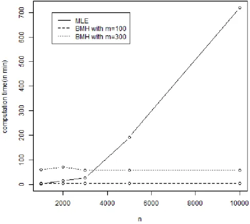
−1.38577 + 5.1541/m . . . 36 4.2 Speed of BMH and MLE with observation size of n: The solid line
represents runing time of MLE in seconds, the dashed line represents the running time of BMH withm= 100, and the dotted line represents the running time of BMH with m= 300. . . 43 4.3 Trace plot of samples of the parameters from the posterior distribution
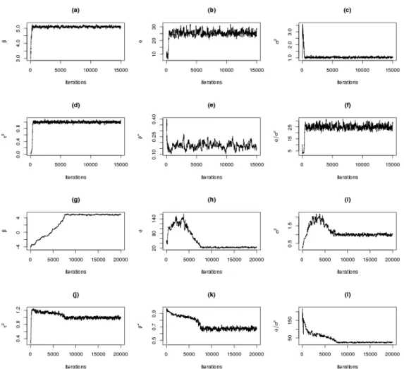
by BMH algorithm: (a)-(f) are trace plots where ρ= 0.2, and (g)-(l) are trace plots where ρ = 0.7. (a)-(f) and (g)-(l) represent β, φ, σ2, τ2, and ρrespectively. . . . . 47 5.1 Total precipitation(left) and Anomalies(right) in April 1948 . . . 51 5.2 Contourplot of April 1948 Anomalies of US precipitation . . . 52 5.3 Trace plot of the parameters in spatial model by BMH algorithm for
April 1984 US precipitation: (a)-(e) represent β, φ, σ2, τ2, and φ/σ2 respectively. The black line is for m = 100, and the red line is for m= 300. . . 53 5.4 Observed and predicted precipitation for April 1948: (a) is the true
values in test dataset, (b) is predicted values of Local Kriging ofδ = 50 with BMH estimator m = 300, and (c) is predicted values of Local Kriging ofδ = 50 with MLE. . . 56
LIST OF TABLES
TABLE Page
4.1 Prameter estimation results of MH and BMH for the simulated ex-ample. The numbers in paranthesis denote the standard deviations of the estimates, which are calculated by average over 10 independent runs. The true value of (β0, β1, β2, β3,logσ2) is (2.0,0.25,0.25,0,-1.3863) 34 4.2 Mean and standard deviations (in the paranthesis) of the estimates
of σ2
11,· · ·, σ552 , σ212 and σ234 obstained by MH and BMH (with k=50 and m/n-bootstrapping) in 10 independent runs, where σ2
ij denotes
the (i, j)th elements of Σ0. . . 37 4.3 Comparison of BMH with D&C and AMHT algorihtms for parameter
estimation, where the numbers in upper row calculated by averaging estimates over 10 runs, and the number in the paranthesis is the stan-dard deviation of the estimates. CPU(sec) is average running time in second. . . 39 4.4 MH, BMH, D&C, and AMHT estimates ofσ112 ,· · · , σ552 , σ212, σ234, and
ρβ2,β3 obtained with pooled samples, where σ 2
ij denotes the (i, j)th
element of Σ0, andρβ2,β3 denotes the correlation coefficient ofβ2 and β3 39 4.5 Comparisons of BMH with MLE for 50 simulated datasets. n: size
of dataset, m: size of subset, CPU(m): averaged CPU time(in min-utes). The numbers in the parenthesis denote the standard error of the estimates. . . 42 4.6 BMH result for the spatial-temporal model with nugget effect: The
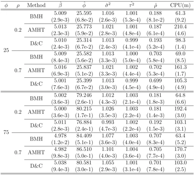
first column,ρ represents the true values for between time autocorre-lation coefficient. . . 48 4.7 Results for the spatial-temporal model of BMH, AMHT, and D&C
with m = 200 and k = 50. From the left column, φ represents the true values of range parameter,ρrepresents the true values of between time autocorrelation coefficient. CPU(m) is running time in minute. 49 5.1 Parameter estimation for April 1948 US precipitation . . . 52
5.2 Averages of MSPEs using neighborhoods within distancesδ. Numbers in paremthesis are stadard errors of the MSPEs. CPU(sec) represents running time in seconds for calculating single MSPE. . . 55 5.3 Parameter estimation of sptial model for April 1948 Anomalies of US
1. INTRODUCTION
Development of computer technology and fast growing internet have been brought us massive volume of data, such as climate data, biological assay data, website trans-action logs, and credit card records. However, such massive data cannot be practi-cally analyzed by a common personal computer becaue their sizes are too big to fit in a memory or it is too time consuming to be analyzed by current statistical methods. To arrange with this problem, one may consider to use parallel and distributed ar-chitectures, with multicore and cloud computing platforms providing access to many processors simultaneously, but still it is unclear how to apply current statistical meth-ods to the big data with muticore system. Also, an increase in size typically comes with growth in complexity of data structures. Big data have put a great challange on current statistical methodology.
During past few decades, Markov chain Monte Carlo (MCMC) methods have been widely used in statistical data analysis, and they have proven to be a very powerful and typically unique computational tool for analyzing data of complex structure. However, if a size of the data is too big, it is intractable to run MCMC methods on a matter of memory or could be time consuming because it needs a large numeber of iterations and complete scan of the data set for each iteration. This have been a serious problem of Bayesian approach, whose main weapon is MCMC methods, to big data issue even though it is powerful for complex model. Motivated by success of MCMC methods in analysing data of complex structure, we propose in this thesis a bootstrap Metropolis-Hastings (BMH) algorithm that is feasible for big data and workable on parallel and distributed architectures. Basically, process of BMH algorithm follows that of Metpolis-Hastings (MH) algorithm, which is the
general form of MCMC methods. BMH algorithm uses a Monte Carlo average of log likelihoods calculated in certain groups of subsets randomly sampled from the full data set whereas Metropolis-Hastings algorithm uses a log likelihood of the full data set. By taking subsets of data, BMH avoids repeated scan of full data set, and its memory usage can be also controlled.
1.1 Metropolis-Hastings(MH) Algorithm
In a Bayesian approach for data analysis, we investigate posterior distribution of parameters for the model. Letθbe the parameter vector containing set of parameters in the model, and let D be the dataset. Then posterior density is
π(θ|D) = π(θ)f(D|θ) C1
(1.1)
where C1 is constant,π(θ) is prior density of θ, andf(D|θ) is likelihood of the data given the parameter setθ. It is common that we don’t know exact closed form of the posterior density π(θ|D) because it is often hard to find the constant C1 or because the model(likelihood) is too complicated to integrate it so that it is hard to make inferences for the parameter set. In those cases, one can consider generating samples from the posterior density and making inference from the posterior samples. More we sample from the posterior, the better inference we can get. Metropolis-Hastings algorithm gives Markov chain generated from a certain distributoin function, and its steps are following.
1. Set initials for θt
2. Generate candidate ϑ from a proposal density g(·|θt)
3. Accept ϑ with probability of α or reject with remaining probability where α is defined by
α = π(ϑ)f(D|ϑ)g(ϑ|θt) π(θt)f(D|θt)g(θt|ϑ)
(1.2) 4. If the candidate is accepted, set the next value as θt+1 =ϑ, or if it is rejected,
set θt+1 =θt.
5. Repeat Step 2-4 for t = 1,2,· · · , B, so we have B posterior samples θ1,θ2, · · · ,θB.
Even though the posterior samples are not independent since they are forming Markov chain, we can have i.i.d. samples by taking every m samples where m is enough large to have independence betwwen θt and θt+m.
However, still there is an important condition that should be satisfied, that is, π(θ|D) should be possibly evaluated. For the case of big data, it is often too time consuming or infeasible because MCMC take large amount of iterations to guarantee precise inferences from the samples. And also if evaluation of the model is containing an inverse of large matrix, for example multivariate gaussian density, its computa-tional complexity is O(n3) where n is a number of observations. Hence, increase of a volum of the data will cause lack of memory or seriously long running time.
1.2 Advanced Markov Chain Monte Carlo Methods for Big Data
In the literature, there have been a few methods proposed for big data anal-ysis such as the aggregated estimating equation method (Lin and Xi, 2011), the resampling-based stochastic approximation method (Liang et al., 2013), the bag of little Bootstraps (Kleiner et al., 2014), and the approximate Metropolis-Hastings test(AMHT) method (Korattikra et al., 2014). The aggregated estimating equation method employs divide-and-conquer strategy. It is first to compress the raw data
to obtain an approximation to the estimating equation estimator, the aggregated estimating equation estimator, by solving and equation aggregated from the saved low dimensional statistics in all partitions. Liang et al. (2013) proposed a new pa-rameter estimator, maximum mean log-likelihood estimator, for big data problem, and a resampling-based stochastic approximation method for obtaining such an es-timator. The resampling-based stochastic approximation method successfully avoids some difficulties involved in big data problems such as inversion of high dimensional matrix. The bag of little Bootstraps provides an efficient way of bootstrapping for big data estimators which functions by combining the results of bootstrapping mul-tiple small subsets of the big original dataset. We propose in this paper a bootstrap Metropolis-Hastings algorithm that takes advantages of the bag of little Bootstrap and the resampling-based stochastic approximation method. BMH algorithm func-tions by maximizing adjusted posterior that is a proportional to multiplication of mean log-likelihood and prior and uses multiple small bootstrap subsets randomly sampled from the original dataset. In this paper, to show an efficiency of BMH, AMHT and divide-and combind method are implemented, and their results are com-pared with that of BMH.
In Chapter 2, we briefly describe some recent approaches to solve big data prob-lem, and in Chapter 3, we will see steps of BMH algorithm and its implementation on parallel architecture with some theoretical background. In Chapter 4, we will assess and compare performances of BMH, AMHT, and D&C method using simu-lated datasets. In Chapter 5, we will apply thses three methods to real datasets, US monthly total precipication, which is spatial data. Finally, in Chapter 6, we close this paper with breif discussion.
2. SOME STRATEGIES FOR BIG DATA
Laney (2012) defined Big data as follows: ”Big data is high volume, high velocity, and/or high variety information assets that require new forms of processing to enable enhanced decision making, insight discovery and process optimization.” High volume might be explained by large number of observations, high velocity represents fast changing model as time goes, and high variety means that various types of data that needs different approaches to analyze. High velocity and variety cause setting of complex model, and as we briefly said in Chapter 1, Markov chin Monte Carlo is considerably suitable for estimating complex model. Hence, Bayesian approach using MCMC can be one great solution for these types of big data problems.
However, its repeated scan of data makes it computationally too slow to be applied to a data of large amount of observations, which is the case of high volume. In this chapter, we will discuss recent approaches suggested as solutions of big data problems: divide-and-conquer strategy, the approximate Metropolis-Hastings test, a bag of little bootstrap, and a resampling-based stochastic aaproximation.
2.1 Divide-and-Conquer(D&C) Strategy
Lin and Xi (2011) developed a computation and storage efficient algorithm for estimating equation(EE) estimation in massive data set using ”divide-and-conquer” strategy. First, one divides full data set into k partitions, and in each partition parameters are estimated using corresponding partitioned data. Then by discarding original data set, one can gaurantee storage efficiency. Later estimated parame-ters from each partition are gathered to compute aggregated EE, which is weighted average of parameter estimators in each partition. In their paper, Newton Raph-son method is used to find maximum likelihood estimator for parameter
estima-tion of each partiestima-tion, and it is not directly comparable to a bootstrap Metropolis-Hastings(BMH) algorithm, which is bayesian approach. Hence, we brought their strategy, divide-and-conquer, by following steps.
1. Divide given massive dataset D into k random partitions, D1,· · · ,Dk
2. Run MH algorithm using each of partitioned datasets, so we have k chains of θ1,· · · ,θk
3. Calculate θˆi by taking average of the chain in each of partition, i, for i =
1,· · · , k
4. Calculate aggregated estimator ˆθ=Pki=1θˆi/k
Lin and Xi (2011) used Ai = Pn
j=1
∂ψ(xij,θˆi)
∂θ as a weight to calculate weighted
average of ˆθi for i = 1,· · · , k where ψ(xij,θ) is score function to be minimized
and xij is j-th observation in i-th partition. However, we instead set Ai = 1 for all
i= 1,· · · , kpartitions to have simple computation, and MH algorithm will converges to equalibrium distribution whose maxizer satisfies minimizing the score function when uniform prior is used.
2.2 Approximate Metropolis-Hastings Test(AMHT)
Korattikra et al. (2014) proposed the approximate Metropolis-Hastings test(AMHT) method to generate random samples from the posterior distribution of big data. This method basically develop approximation by reformulating the Metropolis-Hastings(MH) test as a statistical decision problem. First, draw random numberu∼Uniform [0,1] and in each of MH iteration, with subsample size of ns, accept the proposalϑ if the
average difference µin the log-likelihoods of ϑ and θt is greater than a thresholdµ0, i.e. compute
µ0 = 1 nlog uπ(θt)g(ϑ|θt) π(ϑ)g(θt|ϑ) , and (2.1) µ= 1 ns ns X i=1
li, where li = logf(xi|ϑ)−logf(xi|θt) (2.2)
Then if µ > µ0, accept the proposal and set θt+1 = ϑ. If µ ≤ µ0, reject the proposal and set θt+1 = θt. This reformation of the MH test makes it easy to
frame it as a statistical hypothesis test, H0 : µ > µ0 vs. H1 : µ < µ0. Given µ0 and a random sampleli1,· · · , lins drawn without replacement from the population {l1,· · · , ln}, if the difference between µ0 and the sample mean ¯l=Pj∈{i1,···,im}lj/m is significantly greater than the standard deviation of ¯l, we can make the decision to accept or reject the proposal confidently. Otherwise, we should draw more data to increase the precision of ¯l, i.e. to reduce the standard deviation of ¯l, until we have enough evidence to make a decision. In summary, withmincreasement of subsample, single iteration of AMHT can be achieved by following steps.
1. Initialize estimated means ¯l ←0 and l¯2 ←0 2. Initialize ns ←0, set Xn=D
3. Draw u∼Uniform[0,1]
4. Draw mini-batch X of size min(m, n−ns) without replacement from Xn and
set Xn←Xn\ X
5. Update ¯l and l¯2 using X, and n
s ←ns+kX k
6. Estimate standard deviation s, where
s= √sl r 1− ns−1 and s = r ¯ l2−(¯l)2 ns (2.3)
7. Compute δ ← 1−φns−1
¯ l−µ0
s
where φk is CDF of the standard Student-t
distribution with k degree of freedom
8. If δ > , goto step 4 and repeat, otherwise goto the next step to have decision making
9. Accept the proposal so that θt+1 ←θ0 if l > µ0¯ , otherwise θt+1 ←θt.
The advantage of this method is that one can make confident decisions with ns ≤ n data points and save computation time. The bias-variance trade-off can be
controlled by adjusting the knob . When is high, one makes decisions without sufficient evidence and introduce high bias. As → 0, one makes more accurate decisions but is forced to examine more data which results in high variance.
2.3 A Bag of Little Bootstrap(BLB) Method
Kleiner et al. (2014) introduced the Bag of Little Bootstrap(BLB), a new proce-dure, which incorporates features of both the bootstrap and subsampling to yield a robust, computationally efficient means of assessing the quality of estimators. BLB is well suited to modern parallel and distributed computing architectures and fur-thermore retains the generic applicability and statistical efficiency of the bootstrap. The BLB fuctions by averaging the results of bootstrapping multiple small subsets of X1, X2,· · · , Xn, which are observed i.i.d. samples drawn from some (unknown)
underlying distribution. More formally, given a subset size b < n, BLB samples k subsets of size b from the original n data points, uniformly at random (one can also impose the constrain that the subsets be disjoint). LetI1,· · · ,Ik⊂ {1,· · · , n}be the
corresponding index multisets (note that kIjk= b,∀j), and let P
(j)
nb =b
−1P
i∈IjδXi be the empirical distribution corresponding to subset j where δXi is an indicator function that has 1 if i ∈ Ij and 0 otherwise. BLB’s estimate of ξ(Qn(P)) is then
given by k−1 k X j=1 ξ(Qn(P (j) nb)) (2.4)
which is simple average of estimators calculated by observations in each subset. 2.4 A Resampling-based Stochastic Approximation(RSA) Method
Liang et al. (2013) suggested a Resampling-based Stochastic Approximation(RSA) algorithm. In this method, at each iteration, a small subsample is drawn from the full dataset, and then the current estimate of the parameter is updated accordingly un-der the framework of stochastic approximation. This method also leads to a general parameter estimation approach, maximum mean log-likelihood estimation(MMLE). The method works by minimizing the Kullback-Leibler divergence,
KL(f, g) =− Z log f(z|θ) g(z) g(z)dz (2.5)
where f(z|θ) is a likelihood function that user specified, and g(z) is unknown true density function. Using subsamples randomly drawn from the given data, D, the Kullback-Leibler divergence can be approximated by
c KL(f, g|D) = C− n m −1 ( n m) X i=1 logf(zi|θ) (2.6)
where C denotes a constant related to the entropy of g(z), and mn
is the binomial coefficient. Then, the stochastic approximation method is used to estimate θ by solving the systems of equation ∂KL(f, g|D)c
∂θ = − n m −1( n m) X i=1 H(θ,z) = 0, where H(θ,z) = ∂logf(z|θ)
∂θ is the first order derivative of logf(z|θ) with respect to θ, and z denotes a random sample drawn from D. Then, assymptotically minimizing
c
KL(f, g|D) is to maximize E(logf(zi1,· · · , zim|θ)) where i1,· · ·, im ∈ {1,· · · , n}. RSA can be achieved by following steps.
1. Draw z from D at random and without replacement. 2. θ(t+12) =θ(t)+at+1H(θ,z)
3. If kθ(t+12)−θ(t)k ≤b then set θ(t+1) =θ(t+12), π
t+1 =πt, otherwise set θ(t+1) =
T(θ(t)) and πt+1 =πt+ 1
where π is number of truncation, T : Θ→K0, K0 is compact subset of Θsuch that initial θ0 ∈K0.
3. A BOOTSTRAP METROPOLIS-HASTINGS(BMH) ALGORITHM
The BLB and RSA brought key idea of the bootstrap Metropolis-Hastings(BMH) algorithm. BMH uses many small size of bootstrap samples and calculate mean log-likelihood with those bootstrap samples, and bring this mean log-log-likelihood into the Metropolis-Hastings algorithm instead of full data likelihood. The BMH algorithm can be describe as follows.
3.1 Algorithm
LetDi denote a bootstrap sample ofD, which is resampled from the full data set
at random and with/without replacement. Letmdenote the size ofDi. If resampling
is done without replacement, Di is called a subsample or mn
-bootstrap sample. Otherwise, Di is calledm-out-of-n bootstrap sample or m/n-bootstrap sample. Let
˜
f(Di|θ) denote a likelihood-like fuction of Di, and define
lm,n,k(Ds|θ) = 1 k k X i=1 log ˜f(Di|θ), (3.1)
wherekdenotes the number of bootstrap samples drawn fromD, andDs ={D1,· · · , Dk}
is the collection of the bootstrap samples. The definition of ˜f(Di|θ) depends on the
feature of D. If the observation in D are independently and identically distributed (i.i.d.), then, regardlessDi is a mn
- or m/n- bootstrap sample, we define
˜ f(Di|θ) = ˜f(x (i) 1 ,· · · , x (i) m|θ) = m Y j=1 f(x∗ij|θ) (3.2) wherex∗ij denotes thej-th element inDi. Sincex∗ij’s are no longer mutually
observations in D are dependent, how to define ˜f(Di|θ) will be discussed in section
3.3.
The BMH algorithm works by iterating between the following steps: 1. Draw ϑ from a proposal distribution Q(θt,ϑ).
2. Draw k bootstrap samples D1,· · · , Dk via mn
- or m/n- bootstrapping. Let Ds={D1,· · ·, Dl}
3. Calculate the BMH ratio:
r(θt,Ds,ϑ) = exp{lm,n,k(Ds|ϑ)−lm,n,k(Ds|θt)}
π(ϑ) π(θt)
Q(ϑ,θt)
Q(θt,ϑ)
4. Set θt+1 ← ϑ with probability α(θt,Ds,ϑ) = min (1, r(θt,Ds,ϑ)), and set
θt+1 ←θt with the remaining probability.
Regarding this algorithm, we have the following remarks:
• In BMH, {θt} form a Markov chain with the transition kernel given by
Pm,n,k(θ, dϑ) = X Ds∈D α(θ,Ds,ϑ)Q(θ, dϑ)ψ(Ds) +δθ(dϑ) 1− X Ds0∈D Z Θ α(θ,D0s,ϑ0)Q(θ, dϑ0)ψ(D0s)dϑ0 (3.3)
where D denote the space of Ds, ψ(Ds) denotes the probability of drawing
Ds, and δθ(·) is an indicator function. For mn
-bootsrapping, ψ(Ds) = mn −k
; and for m/n-bootstrapping, ψ(Ds) = 1/nmk
• Let Pm,n,k,Ds(θ, dϑ) =α(θ,Ds,ϑ)Q(θ,ϑ)+δθ(dϑ) 1− Z Θ α(θ,Ds,ϑ0)Q(θ, dϑ0) ,
denote the transition kernel corresponding to a particular subset data Ds.
Then Pm,n,k(θ, dϑ) can be written as a mixture of Pm,n,k,Ds(θ, dϑ)’s; that is,
Pm,n,k(θ, dϑ) = X
Ds∈D
Pm,n,k,Ds(θ, dϑ)ψ(Ds). (3.4)
• When the observations in D are i.i.d., both the resampling schemes, mn− or m/n− bootstrapping, can be used in BMH. As shown in section 3.3, the two resampling schemes lead to the same stationary distribution of the Markov chain.
• If we define
H(θ|Ds) = −lm,n,k(Ds|θ)−logπ(θ)
which is the so-called energy function of the posterior distribution, then the BMH ratio can be written as
r(θt,Ds,ϑ) = exp{H(θ|Ds)−H(ϑ|Ds)}
Q(ϑ,θ) Q(θ,ϑ)
• The BMH algorithm consists of a few parameters, namely, m, k, and the proposal distribution. The proposal distribution can be chosen as in the Metropolis-Hasting algorithm; that is, choosing an appropriate proposal dis-tribution such that the resulting BMH chain is irreducible and aperiodic, and the BMH moves have a reasonable acceptance rate, e.g., between 0.2 and 0.4
as suggested by Gelman et al. (1996) for conventional MH algorithms. A for-mal statement for the requirement of the proposal distribution will be given in condition (B) of Section 3.3.
Since BMH is proposed for simulations on parallel computers, the parameter k species the number of processors/nodes used in computing the averaged log-likelihood function. Theoretically, a large value of k is preferred. However, an extremely large value of k may slow down the computation due to the increased inter-node communications. In our experience, to achieve a good performance for BMH,k does not need to be very large. Both k = 25 and k = 50 work well for all examples of this paper. The choice of m can depend on the complexity of the model under consideration, in particular, the dimension of θ. In general, m should increase with the complexity of the model.
3.2 Parallel Implementation
We used master/slave apporach. At the begining of the algorithm, The data are read simultaneously at each parallel thread. Initial values and candiates, θt and ϑ,
are generated from the master node, and the master node broadcasts (shares) the parameters to all slave nodes. At each of node, subsampling is done independently and simulatenously, and with the subset samples and parameters broadcasted from the master node, log likelihood-like functions, lm,n,k(Ds|θt) and lm,n,k(Ds|ϑ), are
evaluated. Then, the evaluated lm,n,k(Ds|θt) and lm,n,k(Ds|ϑ) are gathered at
mas-ter node, and at the masmas-ter node, priors and acceptance rate are calculated so we can decide whether the candidates,ϑ, will be accepted or not. Still, all parallel nodes are having the initial values and the candidates, so again the acceptance indicator from the master node is broadcasted to the all slaves. If the indicator is 1 that represents the candidates are accepted, the next values are updated to the candidates at all
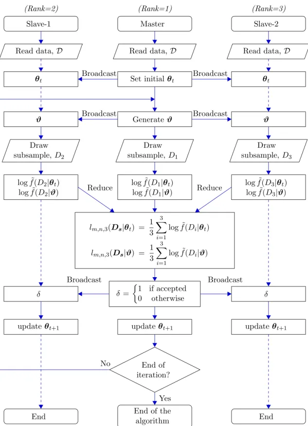
parallel nodes, otherwise, the next values are updated to the current values, and hence, all parallel nodes will be having next values regarded as the initial values for the next iteration. For each of iteration of the BMH algorithm, communications are made up for three times, but actually the communication time is not worrisome be-cause the paralle thereads are communicating only scalar and few parameters which is a vector of short length. Steps for BMH algorithm with parallel implementation is as following. Figure 3.1 shows the following steps on a flowchart.
1. Read data D simultaneously at every parallel thread. 2. Set initial values θt at the master node.
3. Generate the candidates ϑ at the master node.
4. Broadcast θt and ϑ from the master node to the all slaves.
5. Draw random subset Di from the data, D at i-th parallel thread for all i, then
every parallel threads have different random subsets, Ds={D1,· · · , Dk}.
6. At i-th parallel thread, calculate lm,n,k(Di|θt) and lm,n,k(Di|ϑ).
7. Gather lm,n,k(Di|θt)’s and lm,n,k(Di|ϑ)’s, for all i to the master node.
8. At the master node, calculate acceptance ratio, αBM H,and decide wheather ϑ
is accepted or not. If accepted, broadcast δ = 1, otherwise braodcast δ = 0 to all the slaves.
9. At every parallel threads, update θt+1 according to the δ broadcasted from the master node so that θt+1 =ϑ if δ = 1 or θt+1 =θt if δ = 0.
Master Read data, D Set initial θt Generateϑ Draw subsample, D1 log ˜f(D1|θt) log ˜f(D1|ϑ) lm,n,3(Ds|θt) = 1 3 3 X i=1 log ˜f(Di|θt) lm,n,3(Ds|ϑ) = 1 3 3 X i=1 log ˜f(Di|ϑ) δ = 1 if accepted 0 otherwise updateθt+1 End of iteration? End of the algorithm Slave-2 Read data, D θt ϑ Draw subsample, D3 log ˜f(D3|θt) log ˜f(D3|ϑ) δ updateθt+1 End Slave-1 Read data, D θt ϑ Draw subsample,D2 log ˜f(D2|θt) log ˜f(D2|ϑ) δ updateθt+1 End (Rank=1) (Rank=2) (Rank=3) Broadcast Broadcast Broadcast Broadcast Broadcast Broadcast Reduce Reduce No Yes
3.3 Convergence of the Bootstrap Metropolis-Hastings Algorithm
In this section, we first prove the ergodicity of the BMH algorithm and then dis-cuss how to make Bayesian inference for the full dataset based on the BMH samples. The ergodicity of BMH will be studied in two scenarios, namely, mn-bootstrapping and m/n-bootstrapping.
3.3.1 mn
-bootstrapping
To study the ergodicity of BMH, we first assume the following condition holds: (A) sup
θ∈Θ
E|logf(X|θ)|2 <∞
Conditional on the data set D, nlog ˜f(D1|θ),· · · ,f(D˜ k|θ) o
forms a simple ran-dom sample without replacement from a finite population. Motivated by this obser-vation, we deine U-statistic
Um,n(D|θ) = n m −1 X Di∈D h(Di) = X Di∈D log ˜f(Di|θ) (3.5)
whereD is the space ofDi and it contains all the possible mn
subsamples of size m, and h(Di) = log ˜f(Di|θ) is called kernel of the U-statistics. Thus, Um,n(D|θ) is the
conditional mean of log ˜f(D1|θ) on the dataset D. U-statistics were introduced by Hoeffding (1948), which represent a class of statistics that is especially important in estimation theory. Many well known test statistics and estimators, such as mean and variance, are in fact members of this class. The simple structure of U-statistics has made them widely used for studying general estimation processes such as bootstrap-ping and jackknifing, and for generalizing those parts of asymptotic theory concerned with sample means. Refer to Lee (1990) for an overview of theory and practice of
U-statistics. By the law of iterated expectations, it is easy to show that E(lm,n,k(Ds|θ)−Um,n(D|θ))2 =E E((lm,n,k(Ds|θ)−Um,n(D|θ))2|D ≤ m kV ar(logf(X|θ)) (3.6)
which, by condition (A) and Chebyshevs inequality, implies that ask → ∞,n → ∞ and m/k →0,
lm,n,k(Ds|θ)−Um,n(D|θ) p
→0, (3.7)
where→p denotes the convergence in probability. Letgm(D|θ) = exp n
Ehlog ˜f(Di|θ) io
. In the scenario of mn
-bootstrapping for i.i.dobservations, it follows from (3.2) that
gm(D|θ) = exp n
mEhlog ˜f(X1|θ)
io
(3.8)
The variance of aU-statistic based oni.i.d random variables can be expressed in terms of certain conditional expectations. Define for c= 1,2,· · · , m the conditional expectation hc(x1,· · · , xc) = E n log ˜f(X1,· · ·, Xm|X1 =x1,· · · , Xc =xc,θ) o ,
and their variances
σ2c =V ar(hc(X1,· · · , Xc))
Then, according to Hoeffding’s theorem (see e.g., Lee, 1990, p.12),
V ar(Um,n) = n m −1 m X c=1 m c n−m m−c σc2
provided condition (A) holds. Since σ2
c = cV ar(logf(X|θ)) for the U-statistic
de-fined in (3.5), we have
V ar(Um,n) =
m2
n V ar(logf(X|θ)) which implies the following theorem holds:
Theorem 3.3.1 Assume that the condition (A) holds and m =O(nγ), If γ < 1/2, then
Um,n(D|θ)−log(gm(D|θ)) p
→0, as n → ∞ (3.9)
Combining (3.7) and (3.9), we have for anyθ ∈Θ,
lm,n,k(Ds|θ)−log(gm(D|θ)) p
→0, as n→ ∞, (3.10)
where, as implied by (3.7) and Theorem 3.3.1,
m=O(nγ) and k =O(nγ+0) (3.11)
for some 0 >0 and γ <1/2. Define
Γm,n,k(θ,Ds,ϑ) = exp{lm,n,k(Ds|ϑ)−lm,n,k(Ds|θ)} gm(D|ϑ)/gm(D|θ) and λm,n,k(θ,Ds,ϑ) =|log(Γm,n,k(θ,Ds,ϑ))| =|[lm,n,k(Ds|ϑ)−log(gm(D|ϑ))]−[lm,n,k(Ds|θ)−log(gm(D|θ))]|
It follows from (3.10) that λm,n,k(θ,Ds,ϑ) p →0, as n → ∞ (3.12) Define ρ(θ) = 1− X Ds∈D Z Θ α(θ,Ds,ϑ)Q(θ, dϑ)ψ(Ds).
which represents the mean rejection probability of a BMH move starting from θ. To establish the convergence of BMH, we also consider the transition kernel
Pm(θ,ϑ) = α(θ,ϑ)Q(θ,ϑ) +δθ(dϑ) 1− Z Θ α(θ,ϑ0)Q(θ,ϑ0)dϑ0 (3.13)
which is induced by the proposalQ(·,·) for a MH move with the invariant distribution given by
˜
πm(θ|D)∝πm(θ)gm(D|θ) (3.14)
Further, we assume the following conditions hold:
(B) Assume that Pm defines an irreducible and aperiodic Markov chain such that
˜
π(·)Pm = ˜π(·). Therefore, for any starting point θ0 ∈Θ,
lim
t→∞kP
t
m(θ0,·)−π˜m(·)k= 0,
where k·k denotes the total variation norm. (C) For any (θ,ϑ)∈Θ×Θ,
where ψ(Ds) is the resampling probability of Ds from D.
Following from the standard theory of the MH algorithm (see e.g. Tierney, 1994), condition (B) can be simply satisfied by choosing an appropriate proposal distribution Q(·,·). Condition (C) is equivalent to assuming 0 < exp{lm,n,k(Ds|ϑ)
−lm,n,k(Ds|θ)}<∞, which ensures the BMH ratio to be well defined in simulations.
Lemma 3.3.1 states that the kernelPm,n,k, defined in (4), has a stationary
distri-bution. Its proof follows the proof of Lemma 1 (except for some notational changes) of Liang and Jin (2013) for the Monte Carlo MH algorithm, where the MH ratio in-cludes a random quantity calculated using Monte Carlo samples. A similar theorem has also been proved in Adrieu and Robert (2009) for the pseudo-marginal approach, where the likelihood function is approximated using a Monte Carlo approach such as the importance sampling method.
Lemma 3.3.1 Assume conditions (B) and (C) hold. Then for anym, n, k ∈Nsuch that ρ(θ)>0 for all θ∈Θ, Pm,n,k is also irreducible and aperiodic, and hence there
exists a stationary distribution ˆπm,n,k(θ|D) such that for any θ0 ∈Θ,
lim
t→∞kP
t
m,n,k(θ0,·)−πˆm,n,k(·)k= 0.
Lemma 3.3.2 concerns the distance between the kernelPm,n,k and the kernel Pm.
It states that the two kernels can be arbitrarily close to each other, provided that k and n are large enough. The proof can be found in the Appendix.
Lemma 3.3.2 Assume the conditions (A),(B) and (C) hold. If (3.11) holds, then for any ∈ (0,1] and any θ ∈ Θ, there exist N(θ)∈ N and K(θ, n) ∈ N such that
for any φ: Θ→[1,1] and any n > N(θ) and any k > K(θ, n),
|Pm,n,kφ(θ)−Pmφ(θ)| ≤4.
Theorem 3.3.2 concerns the ergodicity of BMH, which states that the kernel Pm,n,k shares the same stationary distribution with the kernel Pm when both n and
k become large. The proof of this theorem follows from the proof of Theorem 1 of Liang and Jin (2013) with some minor changes for accommodating the double limits for k and n.
Theorem 3.3.2 Assume the conditions (A), (B) and (C) hold and the observations are i.i.d. If (3.11) holds, then for any∈(0,1]and anyθ0 ∈Θ, there existN(,θ0)∈
N, K(,θ0, n) ∈ N, and T(,θ0, n, k) ∈ N such that for any n > N(,θ0), k > K(,θ0, n), and t > T(,θ0, n, k)
kPt
m,n,k(θ0,·)−π˜m(·)k ≤,
where π˜m(·) is the stationary distribution of Pm as defined in (3.14).
Theorem 3.3.2 establishes the convergence of BMH under the setting that the bootstrap samples Ds are updated at each iteration. In practice, to avoid frequent
updating of bootstrap samples, one may repeatedly use them for a small number of iterations. This may accelerate BMH, especially when m is large. Letκ0 denote the number of repeated iterations. Following from (3.4), the transitional kernel of BMH for this repeated bootstrap version can be written as
˜ Pm,n,k(θ, dϑ) = X Ds∈D Pκ0 m,n,k,Ds(θ, dϑ)ψ(Ds). (3.15)
Under the same conditions of Lemma 3.3.2, it is shown in the Appendix that
kP˜m,n,kφ(θ)−Pmκ0φ(θ)k ≤4κ0. (3.16)
Hence, the convergence established in Theorem 3.3.2 still follows for the BMH algo-rithm with repeated use of bootstrap samples.
In Section 3.4, we will consider the asymptotics of ˜πm(θ|D). In particular, we
will discuss how ˜πm(θ|D) is related to the whole data posteriorπ(θ|D) asmbecomes
large, and how to make Bayesian inference forπ(θ|D) based on the samples simulated by the BMH algorithm.
3.3.2 m/n-bootstrapping
Under this scenario, the ergodicity of the BMH algorithm can be studied in a similar way to mn-bootstrapping. In what follows, we show with appropriate conditions that BMH has the same stationary distribution for the two bootstrapping schemes. First, we define Vm,n(D|θ) =n−m X 1≤j1,···,jm≤n log ˜f(Xj1,· · · , Xjm|θ)
which is the conditional mean of lm,n,k(Ds|θ) on the dataset D and is called a von
Mises statistic or V-statistic. A straightforward calculation (see the Appendix for the details) shows that
E(lm,n,k(Ds|θ)−Vm,n(D|θ))2 = m k 1− 1 n V ar(logf(X|θ)), (3.17)
which, by condition (A) and Chebyshev’s inequality, implies
lm,n,k(Ds|θ)−Vm,n(D|θ) p
→0, (3.18)
as k → ∞, n → ∞ and m/k → 0. It follows from (3.2) that Vm,n(D|θ) = m
n P
Xi∈Dlogf(Xi|θ). This implies the following theorem:
Theorem 3.3.3 Assume that the condition (A) holds. Let m=O(nγ). If γ <1/2, then
Vm,n(D|θ)−log(gm(D|θ)) p
→0, as n → ∞ (3.19)
Combining (3.18) and (3.19), we have
lm,n,k(Ds|θ)−log(gm(D|θ)) p
→0, as n→ ∞,
under the setting (3.11). Then, by the same reasoning as Theorem 3.3.2, we have the following theorem:
Theorem 3.3.4 Assume that the observations are i.i.d., and the conditions (A), (B) and (C) hold. If (3.11) is satisfied, then BMH with m/n-bootstrapping has the same stationary distribution as with mn-bootstrapping.
3.4 Bayesian Inference
This subsection is organized as follows. In Section 3.4.1, we establish the asymp-totic normality of ˜πm(θ|D). In Section 3.4.2 and Section 3.4.3, we discuss how to
3.4.1 Asymptotic Normality of π˜m(θ|D)
For convenience, we rewrite the full data posteriorπ(θ|D) by πn(θ|D); i.e.,
πn(θ|D)∝πn(θ)f(D|θ),
wheref(D|θ) =Qni=1f(xi|θ) denotes the likelihood function ofD, andπn(θ) denotes
the prior of θ which may depend on the value of n.
The asymptotic normality of posterior distributions has long been studied in the literature. Walker (1969) presented a straightforward approach to the problem for i.i.d. observations. Later, this result was generalized to different statistical models and the conditions were also weakened, see e.g., Dawid (1970), Heyde and Johnstone (1979), and Chen (1985). Among those work, the conditions given in Chen (1985) are very general and flexible. For convenience, we shall present Chen’s result as
√
n(θ(n)−µn)→d N(0,Σ0), (3.20)
whereθ(n) denotes a generic sample of the full data posteriorπn(θ|D),µn denotes a
local mode of πn(θ|D), d
→ denotes convergence in distribution, and
Σ0 =n −∂2logπ n(θ|D)/∂θ∂θT −1 θ=µn = ( −∂2 " 1 nlogπn(θ) + 1 n n X i=1 logf(xi|θ) # /∂θ∂θT )−1 θ=µn
Here, we have assumed that πn(θ|D) satisfies appropriate conditions, to be specific,
the conditions (E1)-(E5) given in Lemma A.0.1 of the Appendix. These conditions re-quire that for eachn,µnis a local maximum ofπn(θ|D) such that∂logπn(θ|D)/∂θ|θ=µ0 =
0 and Σ0 is positive definite, and that for large n, πn(θ|D) becomes highly peaked
and behaves like a normal kernel inside a small neighbourhood of µn, and the prob-ability outside the neighbourhood is negligible. As pointed out by Chen (1985), the posterior πn(θ|D) can be multimodal, and µn does not need to be the global
max-imum. However, the concentration condition must be satisfied at µn; that is, the probability outside a small neighborhood of µn is negligible.
For BMH, lm,n,k(Ds|θ) works as the log-likelihood function, which, as shown
in Sections 3.3.1 and 3.3.2, converges to gm(D|θ) in probability under appropriate
conditions. Let πm(θ) denote the prior distribution of θ. Then the posterior density
function ˜πm(θ|D) is given by ˜ πm(θ|D)∝πm(θ)gm(D|θ) = exp m 1 mlogπm(θ) +Elogf(X|θ) . Let ˜lm(θ) = m 1 mlogπm(θ) +Elogf(X|θ)
. It is assumed that for each m,
(D1) ˜lm(θ) is uniformly continuous on the parameter space Θ, and it has a unique
global maximum and a finite number of local maxima.
(D2) At the global maximum of ˜lm(θ), denoted by µm, the following conditions are
satisfied: (i) ˜l0m(µm) = ∂˜lm(θ)/∂θ θ=µm = 0 (ii) ∂2˜l m(θ)/∂θ∂θT is continuous on Θ, and ˜lm00(µm) = ∂2˜lm(θ)/∂θ∂θT θ=µm is negative definite.
The uniform continuity condition can be satisfied by restricting Θ to a large compact set, say, Θ = [10−100,10100]d, wheredis dimension ofθ. As a practical matter, this is
equivalent to set Θ =Rd. The maxima µ
m. As m → ∞, 1
mlogπm(θ) tends to 0, and thus µm converges to the maximum of
Elogf(X|θ). It follows from Jensen’s inequality that Eθ∗log(f(X|θ)/f(X|θ∗))≤0
for any θ ∈ Θ, where θ∗ denotes the true value of θ and Eθ∗ denotes expectation
with respect to f(x|θ∗). That is, for any θ∈Θ,
Eθ∗logf(X|θ)≤Eθ∗logf(X|θ∗).
Moreover, this inequality is strict unless P(f(X|θ) = f(X|θ∗)) = 1. Hence, as m → ∞, µm will converge to θ∗. The uniqueness condition for the global maximum requires θ∗ to be unique. In the case that the uniqueness condition is violated, e.g., in mixture models, the BMH samples can still be used for model inference after applying a label switching procedure (see e.g., Stephens, 2000). Alternatively, one may impose some constraints on θ such thatθ∗ is unique.
Theorem 3.4.1 shows that under conditions (D1) and (D2), ˜πm(θ|D) will converge
to a normal density function. Its proof can be found in the Appendix.
Theorem 3.4.1 Assume that conditions (D1) and (D2) hold for eachm >0. Then, as m→ ∞, we have
√
m(θ(m)−µm)→d N(0,Σ˜0), as m→ ∞, (3.21)
where θ(m) denotes a generic sample of π˜m(θ|D), and Σ˜0 =m
h
˜l00
m(µm) i−1
.
Let b(θ) be a function of θ. Suppose that ∂b(θ)/∂θ exists and is not 0. Then, by Delta method, we have
√ m(b(θ(m))−b(µm))→d N 0, ∂b(θ) ∂θ T ˜ Σ0 ∂b(θ) ∂θ ! , as m → ∞. (3.22)
Further, by the convergence of the averaged observed information to the Fisher information −1 n n X i=1 ∂2logf(x i|θ) ∂θ∂θT → −E ∂2logf(x|θ) ∂θ∂θT
under regularity conditions, we have
kΣ˜0−Σ0k
p
→0 as n→ ∞ (3.23)
That is, Σ0 can be estimated based on the BMH samples simulated from ˜πm(θ|D).
As implied by (3.21) and (3.23), BMH has the capability to incorporate the whole data information into a single simulation run. Hence, it can have quite different performance from the D&C method. For the latter, suppose that the dataset has been divided into K subsets D1,· · · ,DK, and each is of size m, i.e., n = m×K.
If m is reasonably large, for each subset the corresponding posterior distribution is approximately normal; that is,
√
m(θ(im)−µm,i)→d N(0,Σm,i),
where i indexes the i-th subset, and µm,i and Σm,i denote, respectively, the mean
and covariance matrix of the posterior distribution based on the subset Di . If m is
small, µm,i’s and Σm,i’s can be quite different from others. It is true that µm,i and
Σm,i will asymptotically lose their dependentce on iwhen m becomes large, but this
comes at a price of increasing computational cost. As shown by simulated example in Section 4.1.1, this dependence can lose supprisingly slowly. For a simple linear regression of three predictors, the dependence can still exist for m = 104, see Table 4.4 for the details.
3.4.2 Estimation of the Mean of πn(θ|D)
First, we explore the relationship betweenb(µn) and b(µm). Consider the stan-dard Laplace approximation for posterior means, see e.g., Lindley (1961, 1980), Kass et al. (1990) and Miyata (2004) for the details. Given a prior π, a log-likelihood logp(x|θ), a positive function ξ, and a real functionh, we dene hn and ρ
by hn(θ) = −logp(x|θ)/n−logξ/n and ρ = π/ξ. Suppose that we are interested
in estimating the posterior mean Eπn[b(θ)] for an integrable function b(θ), where Eπn[] denotes expectation with respect to the posterior πn(θ|D). Under regularity conditions, Eπn[b(θ)] can be approximated as follows:
Eπn[b(θ)] = R Θb(θ)ρ(θ) exp{−nhn(θ)}dθ R Θρ(θ) exp{−nhn(θ)}dθ =b(ˆθ) + 1 n X ij bihij ( ρj(ˆθ) ρ(ˆθ) − 1 2 X rs hrshrsj ) + 1 2n X ij hijbij +O(n−2) (3.24) whereρj(ˆθ) = ∂ρ(ˆθ)/∂θj ,bi =∂b(ˆθ)/∂θi,bij =∂2b(ˆθ)/∂θi∂θj,hrsj =∂3hn(ˆθ)/∂θr∂θs∂θj,
hij is the component of the matrix [∂2h
n(θ)/∂θ∂θT]1, and θj denotes the j-th
com-ponent of θ. There are two special cases for the choices of ξ and ρ: If ξ = 1 and ρ = π, then ˆθ becomes the MLE; and if ξ = π, then ρ = 1 and ˆθ becomes the posterior mode.
Suppose thatθ is subject to the following prior:
πm(θ) = [πn(θ)]m/n. (3.25)
Note that this prior setting facilitates the following theoretical analysis, but is not an essential requirement. Then it follows from (3.24) that the posterior meanE˜πm[b(θ)],
which is dened with respect to the posterior ˜πm(θ|D), can be approximated by Eπ˜m[b(θ)] = R Θb(θ)ρ(θ) exp{−mEh(θ)}dθ R Θρ(θ) exp{−mEh(θ)}dθ = R Θb(θ)ρ(θ) exp{−mhn(θ)}dθ R Θρ(θ) exp{−mhn(θ)}dθ =b(ˆθ) + 1 m X ij bihij ( ρj(ˆθ) ρ(ˆθ) − 1 2 X rs hrshrsj ) + 1 2m X ij hijbij +O(m−2), (3.26) where ρj, bi, bij, hrsj, and hij are as defined in (3.24), Eh(θ) = −Elogf(X|θ)−
log(ξ)/n, and the second equality follows from the convergence 1 n n X i=1 logf(xi|θ) a.s. → Elogf(X|θ),
which holds under condition (A). Hence, E˜πm[b(θ)]→b(ˆθ) asm→ ∞. Asn goes to innity, m will also go to innity, then it follows from (3.24) and (3.26) that
Eπ˜m[b(θ)]−Eπm[b(θ)]→0, as m, n→ ∞ (3.27)
and, by setting ξ =π and ρ= 1 in (3.24) and (3.26),
kb(µm)−b(µn)k →0, as m, n→ ∞. (3.28)
Equation (3.27) suggests that we can use the sample average
\ E˜πm[b(θ)] = 1 T T X t=1 b(θt), (3.29)
the approximate posterior ˜πm(θ|D). It follows from (3.27) and the property of
MCMC that Eπ˜\m[b(θ)] provides a consistent estimator forEπn[b(θ)]. Further, it fol-lows from (3.24) and the consistency of MLE that Eπ˜\m[b(θ)] is consistent for b(θ
∗ ); that is, \ Eπ˜m[b(θ)] p →b(θ∗), as m→ ∞. (3.30)
In practice,m cannot be very large for the reason of computational efficiency. As implied by (3.26), we can improve the accuracy of the estimator of b(θ∗) using an extrapolation method by fitting the linear regression
\
Eπ˜m[b(θ)] = β0+β1/m+
for a small set of m, where 1/m works as the explanatory variable, and is the normal random error. Then ˆβ0, the least square estimator of β0, will serve as an estimator of b(θ∗), which corresponds to the limit m→ ∞.
3.4.3 Estimation of the Covariance Matrix of πn(θ|D)
In addition to the mean of the posterior πn(θ|D), the asymptotic covariance
matrix of πn(θ|D) can also be simply estimated based on the BMH samples. It
follows from (3.21) and (3.23) thatmΣˆmprovides a consistent estimator of Σ0, where Σm denotes the covariance matrix of θ(m) calculated based on the BMH samples. In
summary, BMH provides a simple way to asymptotically integrate the whole data information into a single simulation run and thus a convenient way for Bayesian analysis of big data.
4. SIMULATION STUDIES
4.1 A Linear Regression Example Consider the normal linear regression
yi =β0+β1xi1+β2xi2+β3xi3+i, i= 1,· · · , n
where (β0, β1, β2, β3) = (2,0.25,0.25,0) are regression coefficients, and 1,· · · , n are
i.i.d. normal random errors with mean 0 and variance σ2, In simulations, we set n = 105 andσ2 = 0.25, generate bothx1 = (x11,· · · , xn1)T and x2 = (x12,· · ·, xn2)T from the multivariate normal distribution N(0,
boldsymbolIn), and set x3 = (x13,· · · , xn3)T = 0.7x2+ 0.3z, where
boldsymbolIn is an n-by-n identity matrix, and z is also generated from N(0,
boldsymbolIn). Under this setting, x2 and x3 are highly correlated with a theoretial correlation corefficient of 0.919. The high correlation between x2 and x3 makes the posterior distribution πn(θ|D) multimodal and the estimators of β2 and β3 are negatively correlated. Let θ = (β0, β1, β2, β3, σ2) and θ∗ = (2,0.25,0.25,0,0.25) be its true value. We will use this example to demonstrate that (i) BMH can be used for Bayesian analysis of big data; that is, it can correctly estimate the mean and covariance matrix of πn(θ|D), and (ii) the multimodality of πn(θ|D) does not affect
the asymptotically normality of ˜πm(θ|D). For this example, θ∗ is unique, but the
posterior can contain two separated modes.
To conduct Bayesian analysis for this example, we letθbe subject to the following prior distribution πm(θ)∝ 1 σ m/n
as suggested in Section 3.4. To explore the performance of BMH with dierent val-ues of k and m, we tried all cross settings of k = 25,50 and m = 200,500,1000. For each setting of (k, m), BMH was run for 20 times independently; 10 runs for
n m
-bootstrapping and 10 runs form/n-bootstrapping. Each run consisted of 55,000 iterations, where the first 5,000 iterations were discarded for the burn-in process and the samples generated in the remaining iterations were used for parameter estima-tion. To facilitate simulations, we have reparameterized σ2 by log(σ2). Denote the reparameterized parameter vector by ˜θ.
The proposal distribution consisted of two equally weighted components. The first component is designed according to the hit-and-run algorithm (Chen and Schmeiser, 1996), which is to set
˜
θ0 = ˜θt+S×e
where ˜θt and ˜θ
0
denote, respectively, the current and proposed values of ˜θ, e is a random direction drawn uniformly from a unit sphere, and S ∼ N(0, s2). Here s is called the step size of the proposal. The second component is to randomly choose two components of ˜θt to undergo the modication
˜
θ0j = ˜θt,j + ˜e
where ˜θt,j denotes the selected components of ˜θt and ˜e ∼ N(0, s2I2). In all
sim-ulations of this subsection, we set s = 0.15. The resulting acceptance rate of the BMH moves ranges from 0.10 to 0.26 for different values of m. Whenm is large, the posterior distribution becomes highly peaked. To maintain a reasonable acceptance rate, s should be decreased accordingly. For simplicity, we fix s = 0.15 in the every simulations of this section.
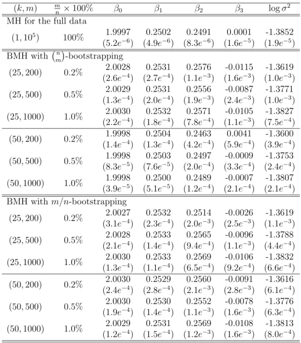
Table 4.1: Prameter estimation results of MH and BMH for the simulated ex-ample. The numbers in paranthesis denote the standard deviations of the esti-mates, which are calculated by average over 10 independent runs. The true value of (β0, β1, β2, β3,logσ2) is (2.0,0.25,0.25,0,-1.3863)
(k, m) mn ×100% β0 β1 β2 β3 logσ2
MH for the full data
(1,105) 100% 1.9997 0.2502 0.2491 0.0001 -1.3852 (5.2e−6) (4.9e−6) (8.3e−6) (1.6e−5) (1.9e−5) BMH with mn-bootstrapping
(25,200) 0.2% 2.0028 0.2531 0.2576 -0.0115 -1.3619 (2.6e−4) (2.7e−4) (1.1e−3) (1.6e−3) (1.0e−3) (25,500) 0.5% 2.0029 0.2531 0.2556 -0.0087 -1.3771
(1.3e−4) (2.0e−4) (1.9e−3) (2.4e−3) (1.0e−3) (25,1000) 1.0% 2.0030 0.2532 0.2571 -0.0105 -1.3827
(2.2e−4) (1.8e−4) (7.8e−4) (1.1e−3) (7.5e−4) (50,200) 0.2% 1.9998 0.2504 0.2463 0.0041 -1.3600
(1.4e−4) (1.3e−4) (4.2e−4) (5.9e−4) (3.9e−4) (50,500) 0.5% 1.9998 0.2503 0.2497 -0.0009 -1.3753
(8.3e−5) (7.6e−5) (2.0e−4) (3.3e−4) (2.4e−4) (50,1000) 1.0% 1.9998 0.2500 0.2489 -0.0007 -1.3807
(3.9e−5) (5.1e−5) (1.2e−4) (2.1e−4) (2.1e−4) BMH withm/n-bootstrapping
(25,200) 0.2% 2.0027 0.2532 0.2514 -0.0026 -1.3619 (3.1e−4) (2.3e−4) (2.0e−3) (2.5e−3) (1.1e−3) (25,500) 0.5% 2.0028 0.2533 0.2565 -0.0096 -1.3788
(2.1e−4) (1.4e−4) (9.4e−4) (1.1e−3) (4.4e−4) (25,1000) 1.0% 2.0030 0.2533 0.2569 -0.0106 -1.3832
(1.3e−4) (1.1e−4) (6.5e−4) (9.2e−4) (6.6e−4) (50,200) 0.2% 2.0030 0.2529 0.2560 -0.0091 -1.3616
(2.4e−4) (2.8e−4) (2.1e−3) (2.8e−3) (6.1e−4) (50,500) 0.5% 2.0030 0.2530 0.2552 -0.0078 -1.3776
(1.9e−4) (1.4e−4) (1.1e−3) (1.6e−3) (6.3e−4) (50,1000) 1.0% 2.0029 0.2531 0.2569 -0.0108 -1.3813
For comparison, Bayesian analysis has also been done for the model using the full dataset with the priorπn(θ)∝1/σ. The MH algorithm was run for 10 times
indepen-dently with the full dataset. Each run consisted of 55,000 iterations, where the first 5,000 iterations were discarded for the burn-in process and the samples generated in the remaining iterations were used for inference. The proposal distribution used in these runs is the same as that used in the BMH runs. Table4.1 compare the pa-rameter estimates produced by MH and BMH. The comparison confirms the validity of BMH: The two resampling schemes, mn-bootstrapping and m/n-bootstrapping, result in almost the same estimates, and the estimates tend to converge to the MH estimates as k and m become large. Note that the standard deviations of the BMH estimates tend to decrease as k and m increase. Table4.1 also shows that BMH is quite robust to the choice of k and m; it can work well with k as low as 25 and a wide range of m.
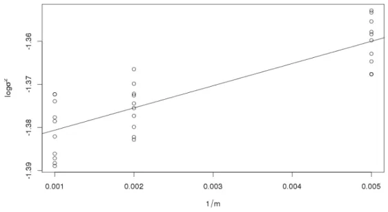
As discussed in Section 3.4.2, the BMH estimates can potentially be improved via extrapolation. To illustrate this procedure, we fit a linear regression for the BMH estiamtes of log(σ2), obtained with (k, m)=(50,200), (50,500), and (50,1000), versus 1/m. Figure 4.1 shows the scatter plot of the BMH estimates and the fitted regression line
\
log(σ2) =−1.38577 + 5.1541/m
whose coefficient of determination is R2=0.7031. The extrapolated estiamte of log(σ2) at m = n is 1.385721, which is surprisingly close to the MH estimate -1.3852.
Next, we explore the estimation of Σ0 , the asymptotic covariance matrix of πn(θ|D), using BMH. To estimate Σ0, we thinned the MH and BMH runs by a factor
Figure 4.1: Regression extrapolation for the BMH estimates of log(σ2) obtained with (k, m)=(50,200), (50,500), and (50,1000): The fitted line is log(σ\2) = −1.38577 + 5.1541/m
of 500 such that the resulting samples are approximately mutually independent. Note that the samples obtained in BMH runs are usually less correlated than those obtained in MH runs, as ˜πm(θ|D) is less highly peaked than πn(θ|D). But, for
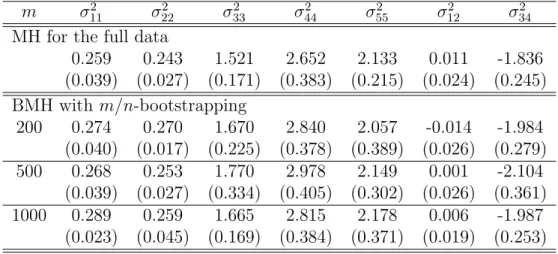
simplicity, we thinned both by the same factor. Table 4.2 summarizes the estimates of Σ0 obtained by MH and BMH (withm/n-bootstrapping and k = 50). The BMH estimates obtained under other settings are similar. In this table, we report the mean and standard deviations of the estimates of σ2
11,· · · , σ255, σ212and σ234obtained in 10 independent runs by the respective algorithms, where σ2
ij denotes the (i, j)th
element of Σ0 . The elements σii, i= 1,· · · ,5, correspond to the posterior variances
of β0,· · · , β3 and logσ2, respectively. The element σ342 corresponds to the posterior covariance of β2 and β3, which are known to be negatively correlated. The element
Table 4.2: Mean and standard deviations (in the paranthesis) of the estimates of σ2
11,· · · , σ552 , σ122 and σ342 obstained by MH and BMH (with k=50 and m/n-bootstrapping) in 10 independent runs, where σ2
ij denotes the (i, j)th elements of
Σ0.
m σ2
11 σ222 σ233 σ442 σ552 σ122 σ342 MH for the full data
0.259 0.243 1.521 2.652 2.133 0.011 -1.836 (0.039) (0.027) (0.171) (0.383) (0.215) (0.024) (0.245) BMH with m/n-bootstrapping 200 0.274 0.270 1.670 2.840 2.057 -0.014 -1.984 (0.040) (0.017) (0.225) (0.378) (0.389) (0.026) (0.279) 500 0.268 0.253 1.770 2.978 2.149 0.001 -2.104 (0.039) (0.027) (0.334) (0.405) (0.302) (0.026) (0.361) 1000 0.289 0.259 1.665 2.815 2.178 0.006 -1.987 (0.023) (0.045) (0.169) (0.384) (0.371) (0.019) (0.253)
σ122 corresponds to the posterior covariance of β0 and β1 , which are known to be uncorrelated. Note that the MH estimate of Σ0 is nΣˆn , and the BMH estimate of
Σ0 is mΣˆm , where ˆΣn and ˆΣm are calculated using the thinned MCMC samples
from their respective runs. Table 4.2 confirms the validity of BMH for Bayesian inference of big data: It can be used through rescaling to quantify the uncertainty of the estimators corresponding to the full data.
4.1.1 A Comparison Study with Existing Methods
In this section, we compare BMH with two existing methods, the divide-and-conquer (D&C) strategy and approximate MH test (AMHT) methods.
As a natural methodology, the D&C method has often been used in big data analysis. The D&C method used in this thesis proceeds as follows.
We first divide the whole dataset into 50 subsets, each consisting of 2,000 obser-vations. The MH algorithm was then run for each subset data for a total of 55,000 iterations, where the first 5,000 iterations were discarded for the burn-in process, and
the remaining 50,000 samples were collected for statistical inference of the model. The proposal used in the simulations was the same as that used by BMH in Section 4.1. The parameters were estimated based on the samples collected from the simu-lations for each subset data. Finally, we combine all the estimates from each subset data by simply averaging to get the final estimate of the parameters. D&C method is also applied to the same cluster architecture that BMH was appled to. After we divide the data set, all process run independently until the final iteration of the chain. So, there are minimum number of comunications between parallel threads. Natually, D&C method takes more computational time with fixed number of parallel threads because it scans 10 times larger number of subjects at every iteration in each group whereas we can fix smaller number of samples, m = 200, for BMH algorithm.
Korattikra et al. (2014) proposed an approximate MH test (AMHT) method for sampling from the posterior distribution of big data. As described in Chapter 2, the significance level controls the approximate accuracy of the posterior distribution and also the proportion of the data to be used at each iteration of the algorithm. To compare AMHT with BMH, we set the mini-batch size m0=200 and tuned the significance level = 0.01 such that around 500 observations, which is 0.5% of the data, will be used at each iteration. Hence, such a run of AMHT cost more CPU time than BMH withm = 200. Note that each run of AMHT employed the same proposal distribution and consisted of the same number of iterations as BMH run. For each run of AMHT, we have also discarded the first 5000 iterations for the burn-in process and used the samples generated in the remaining 50,000 iterations for inference.
Table 4.3 compares the parameter estimates resulted from D&C , AMHT, and BMH (with k = 50, m = 200 and mn
-bootstrapping). BMH can produce very accurate estimates as much as D&C or AMHT, but is much faster than the other two methods although D&C and AMHT involve more observations at each iteration,
Table 4.3: Comparison of BMH with D&C and AMHT algorihtms for parameter estimation, where the numbers in upper row calculated by averaging estimates over 10 runs, and the number in the paranthesis is the standard deviation of the estimates. CPU(sec) is average running time in second.
Algorithm β0 β1 β2 β3 logσ2 CPU(sec)
BMH 1.9997 0.2504 0.2463 0.0041 -1.3600 160.47
(1.46e-4) (1.34e-4) (4.21e-4) (5.90e-4) (3.88e-4) (11.16) D&C 1.9997 0.2503 0.2491 0.0001 -1.3856 238.32
(3.77e-5) (3.40e-5) (5.73e-5) (1.07e-4) (1.33e-4) (10.50) AMHT 1.9999 0.2500 0.2453 0.0050 -1.3716 303.81
(5.47e-6) (6.23e-6) (1.40e-5) (2.02e-5) (2.93e-5) (16.62)
and their standard deviation are smaller than BMH.
In Table 4.4, we report the MH, BMH (withk= 50,m= 200 and mn
-bootstrapping), AMHT (with m0 = 200 and = 0.01), and D&C estimates of σ2
11,· · · , σ255, σ212 and σ2
34 based on the pooled samples from their respective runs, where σij2 denotes the
(i, j)th element of Σ0. For the D&C method, Σ0 was estimated by nkΣˆDC, where ˆΣDC
is the covariance matrix of the posterior samples pooled from 10 runs. For the BMH method, Σ0 was estimated bymΣˆm, wherem = 200 and ˆΣm is the covariance matrix
of the posterior samples pooled from 10 runs. For AMHT method, Σ0 was estimated bynΣˆAM HT, where ˆΣAM HT is the covariance matrix of the posterior samples pooled
from 10 runs. For the MH method, Σ0 was estimated by nΣˆn, where ˆΣn is the
co-Table 4.4: MH, BMH, D&C, and AMHT estimates of σ211,· · · , σ255, σ122 , σ342 , and ρβ2,β3 obtained with pooled samples, where σ
2
ij denotes the (i, j)th element of Σ0, and ρβ2,β3 denotes the correlation coefficient of β2 and β3
Method σ2 11 σ222 σ233 σ442 σ552 σ212 σ342 ρβ2,β3 MH 0.2934 0.2661 1.4488 2.5658 1.9656 0.0580 -1.7657 -0.9158 BMH 0.2746 0.2718 1.6757 2.8428 2.0627 -0.0144 -1.9874 -0.9106 DNC 0.5035 0.5140 3.0750 5.3683 3.8867 0.0093 -3.7258 -0.9170 AMHT 0.3263 0.3788 2.0377 3.1848 2.7706 -0.0056 -2.3386 -0.9180
variance matrix of the posterior samples pooled from 10 runs. As in Table 4.2, the simulations have been thinned by a factor of 500, which ensures the pooled samples to be approximately mutually independent. Table 4.4 shows that BMH can produce correct estimates of Σ0 using pooled samples, while D&C and AMHT cannot.
In summary, BMH can be very efficient for Bayesian analysis of big data, as it is able to incorporate all data information into a single run and thus inference can be made based on a single run. In contract, D&C needs to run for all subsets, otherwise the resulting inference can be severely biased.
4.2 BMH on Spatial Model
In this section, we will assess the performance of BMH algorithm on a spatial model. Consider the Gaussian geostatistical model,
Y=µ+Z+, i.i.d∼ N(0, τ2I) (4.1)
where Y = {Y(s1),· · ·, Y(sn)}T denotes the observations at location s1,· · · , sn,
µ ={µ(s1),· · · , µ(sn)}T denotes the mean vector of Y, Z ={Z(s1),· · · , Z(sn)}T
denotes a Gaussian process with mean, a vector of zeros, and covariance matrix Σ= σ2R, whereRis an exponential correlation function with elements of exp{−ks
i−sjk/φ}
for i, j = 1,· · ·, n where k·k is a distance measure. And τ2 is the nugget variance. The model (4.1) can be extended to the regression setting with the mean µ(si) being
replaced by µ(si) =β0+ p X j=1 βjxj(si) (4.2)
wherexj(·) denotes thejth explanatory variable, andβj is the corresponding
regrre-sion coefficient. Under the model (4.1), Y follows a multivariate Gaussian distribu-tion,Y|θ∼N(µ, σ2R+τ2I), and the log likelihood-like function ofD
is defined as follows. log ˜f(Di|θ) =− n 2log 2π− 1 2log|σ 2R(s i) +τ2I| − 1 2(Y(si)−µ(si)) T σ2R(s i) +τ2I −1 (Y(si)−µ(si)) (4.3)
wheresi is subsample locations of corresponding subsetDi andR(si) = exp{−di/φ}
wheredi is a distance matrix between all locations insi. We suggest following priors
for the model (4.1) with exponential correlation function as non-informative priors.
π(θ)∝
1 φσ2τ2
m/n
50 datasets are generated from the model (4.1) with uniformly distributed spatial sites of size n = 1000, 2000, 3000, 5000, and 10000 respectively. The covariate x
is randomly generated from the normal distribution with mean zero and stadard deviation 0.5. The true parameters for the example are set as β0 = 1.0, β1 = 1.0, φ = 25.0,σ2 = 1.0, andτ2 = 1.0. We set subset size asm= 100 and 300 for each case of n, and the number of subsets is set as k = 50. The length of the Markov chain is 22,000, and the first 2,000-10,000 observations are discarded as burn-in period. The results of our example shows that BMH works very well for estimating the model (4.1). The resulting output is shown in Table 4.5. We took sample means of the chains as the estimators for the parameters. The numbers in Table 4.5 are the averages of the estimates from the 50 datasets, and the numbers in paranthesis are standard errors.
Note that, in this example, asngets bigger, standard errors generally get smaller, and averages of the estimators get closer to the true values. When n is small (n ≤ 1000), MLE is the fastest and the most accurate. However, when n ≥ 2000, BMH
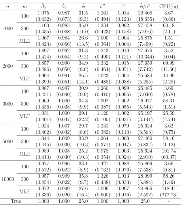
Table 4.5: Comparisons of BMH with MLE for 50 simulated datasets. n: size of dataset, m: size of subset, CPU(m): averaged CPU time(in minutes). The numbers in the parenthesis denote the standard error of the estimates.
n m βˆ0 βˆ1 φˆ σˆ2 τˆ2 φ/ˆˆ σ2 CPU(m) 1000 100 1.075 0.987 31.5 1.261 1.014 29.468 3.67 (0.432) (0.073) (9.3) (0.494) (0.123) (18.655) (0.86) 300 1.103 0.985 35.0 1.334 0.992 27.458 60.18 (0.435) (0.068) (11.0) (0.423) (0.158) (7.976) (2.11) MLE 1.067 0.984 26.6 1.000 1.004 25.875 1.51 (0.423) (0.066) (13.5) (0.364) (0.064) (7.499) (0.22) 2000 100 0.897 0.992 31.3 1.243 1.010 27.676 3.52 (0.424) (0.054) (9.2) (0.490) (0.121) (10.344) (0.04) 300 0.857 0.990 34.9 1.332 1.015 27.659 69.99 (0.486) (0.050) (9.0) (0.464) (0.051) (7.742) (11.66) MLE 0.904 0.991 26.5 1.023 1.004 25.684 14.99 (0.390) (0.051) (14.1) (0.485) (0.038) (5.255) (2.28) 3000 100 0.987 0.997 30.9 1.260 0.999 25.485 3.69 (0.451) (0.040) (9.9) (0.410) (0.095) (7.040) (0.78) 300 0.969 1.000 34.3 1.302 1.002 26.977 58.31 (0.436) (0.038) (9.9) (0.387) (0.055) (5.543) (1.51) MLE 1.031 1.000 29.1 1.120 1.002 25.197 25.59 (0.401) (0.037) (22.2) (0.700) (0.031) (3.141) (4.74) 5000 100 1.024 1.007 29.7 1.231 0.979 25.624 3.62 (0.402) (0.032) (8.6) (0.382) (0.110) (8.563) (0.75) 300 1.044 1.009 33.9 1.264 1.003 27.460 58.16 (0.445) (0.030) (10.3) (0.371) (0.047) (6.834) (1.12) MLE 0.989 1.008 25.2 0.978 1.003 25.624 191.74 (0.413) (0.030) (10.3) (0.354) (0.024) (2.910) (60.37) 10000 100 0.977 0.996 33.1 1.427 0.988 25.809 3.66 (0.572) (0.022) (8.9) (0.732) (0.076) (7.538) (0.81) 300 0.957 0.999 35.8 1.326 1.013 28.099 58.26 (0.454) (0.022) (9.7) (0.438) (0.033) (5.884) (1.49) MLE 0.972 0.999 27.6 1.096 0.997 24.866 718.44 (0.336) (0.020) (16.4) (0.600) (0.016) (2.592) (272.73) True 1.000 1.000 25.0 1.000 1.000 25.0
-with m = 100 gets 5 to 200 times faster than MLE. For the cases of BMH with m = 300, when n ≥5000, BMH gets faster than MLE. It is because computational complexity of BMH, which is O(m3), is independent of n, whereas that of MLE is O(n3). Whatever the size of n is, the computation time of BMH is constant for fixed subsample size m. When the number of observation gets larger, it is getting hard to get MLE in matters of memory and speed, but there is still no problem in calculating BMH estimator. BMH could be more powerful for more complex
Figure 4.2: Speed of BMH and MLE with observation size of n: The solid line represents runing time of MLE in seconds, the dashed line represents the running time of BMH withm= 100, and the dotted line represents the running time of BMH with m = 300.