JOURNAL OF IEEE TRANSACTIONS ON AFFECTIVE COMPUTING
Improving attention model based on cognition
grounded data for sentiment analysis
Yunfei Long, Xiang Rong, Qin Lu, Chu-ren Huang, and Minglei Li
Abstract—Attention models are proposed in sentiment analysis and other classification tasks because some words are more important than others to train the attention models. However, most existing methods either use local context based information, affective lexicons, or user preference information. In this work, we propose a novel attention model trained by cognition grounded eye-tracking data. First,a reading prediction model is built using eye-tracking data as dependent data and other features in the context as independent data. The predicted reading time is then used to build a cognition grounded attention layer for neural sentiment analysis. Our model can capture attentions in context both in terms of words at sentence level as well as sentences at document level. Other attention mechanisms can also be incorporated together to capture other aspects of attentions, such as local attention, and affective lexicons. Results of our work include two parts. The first part compares our proposed cognition ground attention model with other state-of-the-art sentiment analysis models. The second part compares our model with an attention model based on other lexicon based sentiment resources. Evaluations show that sentiment analysis using cognition grounded attention model outperforms the state-of-the-art sentiment analysis methods significantly. Comparisons to affective lexicons also indicate that using cognition grounded eye-tracking data has advantages over other sentiment resources by considering both word information and context information. This work brings insight to how cognition grounded data can be integrated into natural language processing (NLP) tasks.
Index Terms—Affective lexicons, Sentiment analysis, Cognition grounded data, Deep learning, Attention model
F
1
INTRODUCTION
Sentiment analysis is critical for many applications such as opinion based product recommendation [1], public opinion detection [2], and affective human-machine interaction [3], etc. Sentiment analysis has been studied extensively using different methods applied on different types of data [4], [5], [6], [7], [8]. Many approaches are used in sentiment analysis tasks such as lexicon based statistical methods, rule based methods, and linear classification methods [4], [9]. Deep learning based methods in recent years have further elevated the performance of sentiment analysis without the need for labor intensive feature engineering [6], [10].
Research in cognitive studies have indicated that not all words contribute equally in the semantic and affective meaning of a sentence [11]. Some words are more im-portant than others in conveying messages in sentences. Similarly, some sentences are more important than others in a document.In text classification tasks, attention models are proposed to give different weights to different words in text. Attention models are also incorporated into deep • Y.Long is with the Horizon Digital Economy Research Institute, Univer-sity of Nottingham, Nottingham, UK. The work was done when he was a PhD student with in the Hong Kong Polytechnic University.
E-mail: [email protected];
• R. X, Q. Lu are with the Department of Computing, The Hong Kong Polytechnic University, Hung Hom, Kowloon, Hong Kong.
E-mail:{csxiang,csluqin}@comp.polyu.edu.hk;
• C. Huang with the Department of Chinese and Bilingual Studies, The Hong Kong Polytechnic University, Hung Hom, Kowloon, Hong Kong. E-mail:[email protected];
• M.Li is with the Department of Computing, The Hong Kong Polytechnic University, Hung Hom, Kowloon, Hong Kong.
E-mail: [email protected];
Manuscript received November 23, 2017; revised December 12, 2018; Accepted February 28, 2019.
learning based sentiment analysis models. Reading time is one important measure used in cognitive studies. Al-though the overall reading time in a cognitive process may reflect the syntax and discourse complexity, reading time of individual words is also an indicator of their semantic importance in text [12]. Previous attention models are built using information embedded in text including users, prod-ucts and text in local context for sentiment classification or other downstream tasks [7], [10], [13], [14] [15]. However, attention models using local context based text through distributional similarity lack theoretical foundation to reflect the cognitive basis. But, the key in sentiment analysis lies in its cognitive basis [16].
Two phenomena rally behind the cognitive theories of sentiment analysis [17]. First, people react to the same event with a variety of different emotions. The reaction is subjected to individuals’ biases based on their cognitive experiences. Second, different events may trigger the same emotion as there are only a number of emotional reactions cognitively. We envision that cognition grounded data ob-tained in text reading should be helpful in building an attention model.
In this paper, we propose a novel cognition grounded attention (CGA) model for sentiment analysis learned from cognition grounded eye-tracking data. Eye-tracking is the process of measuring either the point of gaze or the motion of an eye relative to the head 1. Psycho-linguistics
exper-iments, [18] show that readers are less likely to fixate on close-class words that are predictable from context. Readers also fixate longer on words which play significant seman-tic roles [12] in addition to infrequent words, ambiguous words, and morphologically complex words [19]. Since
reading time can be learned from an eye-tracking dataset, predicted reading time of words in its context can be used as indicators of attention weights.
In this work, we first build a regression model to map lexical, syntax, and context features of a word to its reading time based on eye-tracking data. We then apply the model to sentiment analysis datasets to obtain estimated reading time of words at the sentence level. The estimated reading time then used as the attention weights in its context to build the attention layer in a neural network based sentiment anal-ysis model. Evaluation on five sentiment analanal-ysis related text classification benchmark datasets (IMDB, Yelp 13, Yelp 14, IMDB2 and Fake) show that our proposed model can significantly improve the performance compare to the state-of-the-art attention methods. We also compare the effect of eye-tracking based CGA to other lexicon based attention mechanism based on the lexicon work of [20]. Results also show that eye-tracking based CGA can contribute to higher performance gains than attention models build by other lexical based sentiment resources. This is mainly because our attention models are based on context dependent in-formation whereas lexicon based resources are static, and context information are not included.
To sum up, we have three major contributions: First, we propose a novel cognition grounded attention model to improve the state-of-the-art neural network based sen-timent analysis models by learning attention information from eye-tracking data. This is a novel attempt to use cognition grounded data in deep learning based sentiment analysis. The CGA model not only can capture attention of words in their context at the sentence level, it can also be aggregated to work at the document level. CGA can also be incorporated with other attention mechanisms to capture other aspects of attentions. Secondly, evaluation on several real-world datasets on sentiment analysis shows that our method outperforms other state-of-the-art meth-ods significantly. Our evaluation also include comparing to several lexicon based sentiment resources. Even though, most of the lexicon based sentiment resources can help to build attention based sentiment analysis model, they simply cannot match up to the perform improvement brought up by using eye-tracking data in our proposed framework. This work validates the effectiveness of cognition grounded data in building attention models. More importantly, we bridge the gap between sentiment analysis and cognitive process by using cognition grounded data to build attention model and subsequently improve sentiment analysis models. We prove the indirect connection between cognition grounded data and sentiment can be modeled to improve sentiment analysis under attention mechanism.
The rest of the paper is structured as follows: Section 2 describes related works, including document classification and sentiment analysis, eye-tracking data, and other lexicon based resources. Section 3 introduces our proposed method for improving attention model based on cognition grounded data. Section 4 performs extensive experiments on various sentiment analysis related dataset to validate the effective-ness of our proposed method. Section 5 concludes this paper and discuss future works.
2
RELATED
WORKS
Our proposed work aims to solve document level sentiment analysis problem, Previous related include using attention model for sentiment analysis, building attention mechanism based on local semantic or external user information. Be-cause we aim to incorporate cognition ground data into sentiment analysis model, we also introduce previous works using cognition grounded data and other lexicon based sentiment resources.
2.1 Sentiment analysis
The basic task in sentiment analysis can be formulated as a classification problem. Class labels can either be discrete (positive/negative) or continuous (for example, ratings in certain range such as 0 to 5 or 1 to 10, etc.). Generally speaking, three different levels of sentiment analysis can be performed depending on granularities. The first isdocument level sentiment analysis. The second issentence level sentiment analysis. In this level, polarity is calculated for each sentence as each sentence is considered a separate unit and different sentences can have different opinions. The last level isfeature level sentiment analysis. The task of feature level sentiment analysis is to identify the piece of text as an aspect of some products [21]. Typical feature level task is aspect based sen-timent analysis [22]. Our paper targeted to solve document level sentiment analysis problem. The same approach can also applied to other level of classification tasks with minor modification.
The first works in sentiment analysis are based on lexical rules. Hatzivassiloglou et al. [23] proposed a sentiment anal-ysis task explicitly based on the adjectives, present in the English linguistic resources. The proposed linguistic rules based on 21 million words of English. Rule based methods are simple but lack of generalization ability. Later works in sentiment analysis based on linear classifier with feature engineering. Support Vector Machine (SVM) classifier has achieved great success in text classification [4], [24]. SVM with effective feature engineering was considered com-monly used sentiment classification methods before deep learning methods came out.
In recent years, deep learning based methods have greatly improved the performance of sentiment analysis. Commonly used models include Convolutional Neural Networks (CNN) [25], Recursive Neural Network (ReNN) [26], and Recurrent Neural Networks (RNN) [27]. RNN nat-urally benefits sentiment classification because of its ability to capture sequential information in text. However, standard RNN suffers from the so-called gradient vanishing problem [28] where gradients may grow or decay exponentially over long sequences. To address this problem, Long Short Term Memory model (LSTM) is introduced by adding a gated mechanism to keep long term memory. Each LSTM layer is generally followed by mean pooling and then feed into the next layer. Experiments in datasets which contain long documents and long sentences demonstrate that LSTM model outperforms the traditional RNN [6], [29] in most of document level sentiment analysis tasks. To include larger scope of information, memory network [30], [31] is used into sentiment analysis [32], [33]. Memory network models
have achieved the state-of-the-art results in aspect level sentiment analysis [34].
Not all words contribute equally to the semantics of a sentence [35]. Attention based neural networks are pro-posed to highlight their difference in contribution [36]. In document level sentiment classification, both sentence level attention and document level attention are proposed. In sen-tence level attention layer, an attention mechanism identifies words that are important. Those informative words are ag-gregated as attention weights to form sentence embedding representation. This method is generally called local context based attention method. Similarly, some sentences can also be highlighted to indicate their importance in a document. The recent models are proposed to build attention model in the multiple aspects of context information [37].
Apart from local context attention, for product review text, user/product attentions are also included in deep learning methods either in a separate network [13] or in a unified network [29]. Some feature engineering methods to some specific datasets can also achieve very good result [38] especially in competition tasks. The methods to use user profile as attention mechanism also expands from sentiment analysis to other document classification tasks, such as fake news detection [39]. However, they are not suited for other genre of text as user-product information are not generally available.
An important issue in all levels of sentiment analysis is how to incorporate affective lexicons in a sentiment analysis model, especially under the deep learning framework. Dong et al. [40] proposed a sentiment parser to analysis how sentiment changes when a phrase is modified by negators or intensifiers. Another approach takes special lexicons as reg-ularization factors in the loss function of Deep learn model. This can be seen in Yogatama et al. [41] introduces three linguistically motivated structured regularizers [42] based on parse trees, topics, and hierarchical word clusters for text categorization. This paper applies group lasso regularizers to logistic regression on model parameters. Qian et al. [43] takes a different approach which attempt to model the linguistic role of sentiment lexicons, negation words, and in-tensity words as intermediate outputs with KullbackLeibler divergence 2. But the use of lexicons still limited to use
certain type of words from a sentiment lexicon. Cognition grounded data like eye-tracking and electroencephalogra-phy (EEG) data are rarely incorporated in sentiment analy-sis. Mishra et.al [44], [45], [46] propose a multi-task deep neural framework for document level sentiment analysis to predict the overall sentiment expressed in a document. multiple tasks include the learning of human gaze behavior and auxiliary linguistic tasks like part-of-speech tagging, detecting syntactic properties of words, or finding sarcastic information in the document. However, this model needs gaze information to be available in the sentiment analysis dataset. Gathering information for large sentiment datasets is too labor expensive.
2.2 Cognition grounded data
Eye-tracking data is one of the most commonly used cogni-tion grounded data [47]. In the simplest terms, eye-tracking
2. https://en.wikipedia.org/wiki/Kullback-Leibler-divergence
measures eye activity. Eye-tracking data is collected using either a remote or head-mounted tracker device connected to a computer. Although it is novel to use eye-tracking for attention based sentiment analysis model, there are some researches connecting eye-tracking with sentiment analysis. Joshi et al. [48] proposes a novel metric called Sentiment Annotation Complexity for measuring sentiment annotation complexity based on eye-tracking data. Another research [49] presents a cognitive study of sentiment detection from the perspective of artificial intelligent where readers are tested as sentiment readers. Mishra et al. [50] recently pro-poses a model in sentiment analysis and sarcasm detection by using eye-tracking data as a feature in addition to text features using naive-bayes (NB) and support vector machine (SVM) classifiers.
In other NLP tasks, Joshi et al. [51] shows that word-sense-disambiguation (WSD) can make use of simultaneous eye-tracking. Eye-tracking data are also used to measure the difficulty in translation annotation [52]. Barrett et al. [18] finds that gaze patterns during reading are strongly influ-enced by the role a word plays in terms of syntax, semantic, and discourse. Mishra et.al [45] introduce a novel method to predict sarcasm understandability based on distinctive eye-movement behavior by human readers.
Even though psycholinguistics has studied the relation-ship between eye-tracking and sentiment for a long time, it is novel to use cognition grounded data in sentiment analysis from deep learning perspective.
Among different available eye-tracking datasets, the Dundee corpus, GECO (the Ghent Eye-Tracking Corpus), and Mishra et al. [50] are considered as high-quality re-sources [50], [53], [54]. The Dundee corpus contains eye movement data from English and French newspapers [53]. Measurements are taken while 10 participants read 20 news-paper articles. GECO is an English-Dutch bilingual corpus with eye-tracking data from 17 participants collected from reading the complete novel The Mysterious Affair at Styles. The corpus has 4,934 sentences, 774,015 tokens, and 9,876 words. The Mishra [55] dataset contains 994 text snippets with 383 positive and 611 negative examples from newspa-per clippings, sampled from seven native speakers.
To predict human reading behaviors, Tomanek et al. [56] proposes a regression model using linguistic features related to syntax and semantics for calibration. Hahn et al. [35] proposes a novel approach to model both skipping and reading using unsupervised method which combines neural attention with auto-encoding trained on raw text using reinforcement learning. This model is compared with previous supervised models in modeling reading behavior and human Performance baselines.
2.3 Other Affective Lexicons
Based on different models, sentiment lexicons are built either using a discrete affective model (such as happiness, sadness, fear, surprise, etc.) or a continuous model (e.g. ranging positive score from 0-1 or 1-5 3) [20]. Affective
3. For example, Evaluation-Potency-Activity (EPA) using continuous values for each dimension range from 1-5. For example, under a common culture environment,mother is represented as e: p: a of 2.9; 1.6; 0.5, enemy is represented as e: p: a of 2.1; 0.8; 0.2
lexicons,if they take discrete values, are multi-labeled. But they can easily be projected into binary polarities. And thus can also be used as sentiment analysis resources. For affective lexicons in multidimensional space, their mapping to sentiment space can also be done easily and thus, we general refer to the resources as affective lexicons. Because eye-tracking data provide word in one dimensional with continuous values, we will only focus on continuous based lexicons in this work. Theoretically speaking, methods to obtain a sentiment lexicon can be extended to obtain other affective lex.
Affective lexicons can be obtained either by manual annotation (include but not limited to crowdsourcing)or au-tomatic methods.Manual annotationcan obtain high-quality lexicons. Manually annotated sentiment lexicons include the General Inquirer (GI) [57], MPQA [58], the twitter sentiment lexicon [59], [60], VADER [9], etc.
Manually annotated multi-dimensional lexicons in other affective dimension include ANEW, CVAW, DAL, EPA and ANGST, etc. The ANEW lexicon is based on a three dimension model on Valence, Arousal, and Dominance (VAD) model [61] which contains 1,034 English words. Valence can directly serve as the sentiment dimension. The extended ANEW lexicon contains about 13,965 English words annotated through crowdsourcing. The CVAW lex-icon based on the VAD model [62] contains 1,653 tradi-tional Chinese words in the valence and arousal dimen-sions. The Dictionary of Affect in Language (DAL) lexicon annotated in the dimensions of Pleasantness-Activation-Imagery contains 8,742 terms [63]. Pleasantness can directly serve as the sentiment dimension. The Evaluation, Potency, and Activity (EPA) lexicon annotated in the evaluation-potency-activity dimensions [64] contains about 4,505 En-glish terms. Here the evaluation dimension is close to sen-timent in the EPA schema. The ANGST lexicon annotated in the valence(sentiment)-arousal-dominance-imageability-potency dimensions contains 1,003 German words [65]. But the biggest problem for manual annotation is high costs in both time and resources. Hence most of manually annotated resources is limited in size.
Given the limitation of manually labeled resources, re-searches start to apply automatic methods to build lexicon. Automatic methods to obtain affective lexicons are focused mainly on the sentiment space because current research works are mostly on sentiment analysis [66], [67], [68] [20]. In terms of methodology, there are mainly three approaches. The first approach uses statistical information between a target word and seed words. For example, sentiment po-larity intensities are calculated based on Point-wise Mutual Information (PMI) between a target word and positive seeds and negative seeds, respectively [59], [69]. Similarly, PMI is used to build discrete emotion lexicon based on naturally annotated hashtags in twitter [70]. The second approach is based on label propagation method which firstly builds a word graph and then label propagation is performed to infer the affective values of unseen words from the seed words. For example, a graph can be built based on the semantic relationship in WordNet and the label propagation is performed to infer the EPA values [71] and sentiment polarity [72]. A knowledge based graph is confined by the coverage of a knowledge base. A word graph can also
be built from a text corpus based on cosine similarity of words represented by their contexts words and then graph propagation is performed to infer the sentiment polarity of unseen words [73]. Word embedding is also used to compute cosine similarity between words to build the word graph [74]. Similarly, a word graph is constructed using cosine similarity of word embedding to infer sentiment polarities [68]. The third approach represents a word as a vector and then map this vector to some sentiment value or categories based on a regression model or a classifier. Features used in vectors can be either manual defined or by expert knowledge. Then features are processed by linear regression to obtain sentiment labels or scores [75] [76]. A recent work proposed by Li et al. [20] proposed a Ridged regression based methods to inferring affective meanings of words from word embedding. Evaluation on various affective lexicons shows that ridge regression outperforms the state-of-the-art methods on all the lexicons under dif-ferent evaluation metrics with large margins. The works conducted by Li et al. [20] also provide several large scale affective lexicon for public use.
3
PROPOSED
METHOD
The design principle of our method is to add a CGA (Cog-nition Grounded Attention) model into a neural-network based LSTM sentiment classifier, a classifier that gives the state-of-the-art performance in sentiment analysis [77]. Let
Dbe a collection of documents. A documentdk,dk ∈D, has
msentencesS1, S2, ...Sj, ..., Sm. A sentenceSjis formed by a sequence of wordsSj =w1jw
j 2...w
j
lj, whereljis the length
ofSj. The features of a wordwi ∈Dform a feature vector
~vwi = [F1
wi, F
2wi....Fnwi]wherenis the feature space size. The purpose of document level sentiment classification is to project a document dk into the target space of L class labels. Similarly, at the sentence level, the purpose is to map a sentenceSj into the target class space.
To build the CGA model, we need to first build a reading time prediction model for words within each sentence. Reading time is predicted based on word features and text features calibrated by eye-tracking data. Note that reading time from an eye-tracking dataset cannot be used directly because the text of any eye-tracking dataset is too small for sufficient coverage. Consequently, our method has four tasks: (1) to predict the reading time of words using eye-tracking data with ~vwi as features; (2) to build attention
models based on predicted reading time at sentence level and document level; (3) to integrate the proposed attention model with other attention models; and (4) to add the attention models into a LSTM based sentiment classifier.
3.1 Modeling of reading time
To learn the reading time of words in a sentence, our method is based on regression analysis using eye-tracking data as dependent variables and context information in
~vw∈Sjas independent variables. In the eye-tracking process,
a number of different time measures are included such as first fixation duration,gaze duration, andtotal reading time. In this work, we only usethe total reading time.
We use features extracted from the context of an eye-tracking corpus to train the regression model. We select fea-tures based on the works from Demberg [12] and Tomanek [56] to include word features such as word length and POS tags as well as context level syntax and semantic features such as the total number of dominated nodes in a depen-dency parsing three, the maximum dependepen-dency distance, semantic category etc..
The features we selected are in four groups:
• Morphology features: number of characters and words per annotation phrase; words in a phrase start with capital letters; words in a phrase consist of capital letters words which only have alphanumeric characters, or words which have punctuation sym-bols.
• Character features: number of named entity words and percentage of named entity words in the anno-tation phrase.
• Complexity features: syntactic complexity: number of dominated nodes, part-of-speech (POS), n-gram probability,maximum dependency distance; seman-tic complexity: inverse document frequency; ambigu-ity (number of senses); general linguistic complexambigu-ity: Flesch-Kincaid Readability Score
• Context features: named entities in word context (preceding or following current phrase); abbreviation in word.
Given a wordwin a sentenceSj,w∈Sj, and its feature vector~vw∈Sj = [F
w
1 , F2w, ..., Fnw], the regression model on eye-tracking data is a mapping functiongbetween reading timetw∈Sj and~vw∈Sj as defined as follows:
tw∈Sj =g(α1F
w
1 +α2F2w+...+αnFnw+b), (1) where tw∈Sj is the predicted reading time for w, αi
is the weight of feature Fw
i , and b is a constant. Note that the set of αi(i = 1...n) forms the weight vector ~αw for tw∈Sj. When ~vw∈Sj takes scalar values, g can be an
identity function and thus this model becomes a typical linear regression model. Whentw∈Sj takes discrete values, gcan be a logistic function and this model becomes a typical logistic regression model.
We setgto be the identity function. A objective function then becomes: min ~ α n X ai∈~α ||tw∈Sj−yw∈Sj|| 2 2+λR(~α), (2) where yw∈Sj is the true eye-tracking values of reading
time,R(~α)is the regularization ofα~, andλis the regular-ization weight. Whenλ= 0, the model degrades to a linear regression function. In this work, we evaluate the use of both the linear regression model and the Ridge regression model.
3.2 Building the attention based model
Once we have the predicted reading time for each words used in sentences, the attention model can be built with two components. The first component works at the sen-tence level to give different words different emphasis in a
sentence. The second component works at the document level to give different sentences different emphasis in a document.
For a sentenceSj =w1w2...wi...wlj with lengthlj, each
wordwiinSjhas a corresponding reading timetwi. LettSj
denote the total reading time ofSj. Then,
tSj =
lj X
i=1,wi∈Sj
twi. (3)
For sentence level attention, the CGA (Cognition Grounded Attention) weight forwiinSj, denoted asASj:wi,
can be defined as:
ASj:wi= twi tSj
. (4)
This sentence level attention model defined above gives more weights to words that have longer reading time rela-tive to the total reading time of the sentence.
Let a document dk, dk ∈ D, be formed by a set of m sentencesSj=w1w2...wi...wlj. Now the CGA weight for a
sentenceSj indkis defined as:
Adk:Sj = tS
Pm
i=1tSi
. (5)
This aggregated document level attention model gives more weights to the sentences that have longer reading time relative to the total reading time of the document. LetA~dk
denote the document level attention weight vector. The size ofA~dkshould bem, the number of sentences indk.
Let S~j denote the embedding of Sj in N dimensional space, whereSj ∈dk. Then, the set of sentence representa-tions fordk(containmsentences) should be a matrix of size
m×N, denoted bySˆdk. After the inclusion of the attention
model,Sˆdkshould be: ˆ
Sdk=A~dkS~
T
j. (6)
Letd~k denote the document embedding ofdk. Sinced~k is anN dimensional vector,d~k can now be defined by the adjusted attention model as:
(d~k)i= m
X
j=1
( ˆSdk)i,j. (7)
3.3 Incorporation of other attention models
Since document embedding representation allows com-bined use of multiple attention mechanisms, it is to our advantage to incorporate different attention mechanisms to help in capturing different aspects of attentions. Generally speaking, different attention mechanisms can be incorpo-rated either serially or in parallel.
In principle, any number of attention models can be included. As an example to illustrate the capability of our proposed method, we choose one state-of-the-art local attention model (shorthanded as LA) as an example for inclusion. The model is a semantic-based local attention model proposed by Yang [36] and also used by Chen [7]. For inclusion serially in the LSTM layer, the attention weight is formulated as follows:
AsSj:wi=LASj:wi∗ASj:wi, (8)
whereLAsj:wi is the sentence level attention model by the
Yang et al.’s [36] local attention model.
To incorporate LA in parallel mode, the attention weight can be formulated by:
ApSj:wi=LASj:wi+ASj:wi. (9)
Similar methods can be used at document level.
3.4 General sentiment analysis model
We take the neural network based LSTM sentiment classi-fier [78] to be applied at both the sentence level and the document level because of its excellent performance on long sentences [6]. The basic LSTM model has five internal vectors for a nodeiincluding an input gate~ii, a forget gate
~
fi, an output gate o~i, a candidate memory cell ~c0i, and a memory cell~ci,~iif~iando~iare used to indicate which values will be updated, forget or for keeping in the LSTM model.
~c0i and~ci are used to keep the candidate features and the actual accepted features, respectively.
At the sentence level, each wordwi in a sentenceSj is represented by its word embedding w~i in N dimensional space. The LSTM cell state~ci and the hidden state~hSj:wi
can be updated in two steps. In the first step, the previous hidden state~hSj:wi−1 uses a hyperbolic function to form~c
0 i as defined below.
~
c0i=tanh( ˆWc∗[~hSj:wi−1∗w~i] + ˆb), (10) where Wˆc is a parameter matrix,~hSj:wi−1 is the previ-ous hidden state and w~i is the word vector.ˆb is the bias parameter matrix.
In the second step,~ci is updated by~c0i and its previous state~ci−1to form~ciaccording to the below formula:
~ci=f~i∗~ci−1+i~i∗~c0i. (11) The hidden state ofwican be obtained by
~hSj:wi=o~itanh(f~i∗~ci). (12)
The forget gate f~i is designed to keep the long term memory. A series of hidden states ~h1~h2...~hi can serve as input to the attention layer to obtain sentence representation
~
Sj. In the document level, similar method is used to get the sentence matrixSˆin the document level LSTM layer to obtain the final document representationd~k.
In our work, the final document representation d~k en-codes both sentence level information and document level information. In the LSTM model, we use a hidden layer to project the final document vector d~fk through a hyperbolic function.
~
dkf =tanh( ˆWhd~k+ ˆbh), (13) whereWˆh is the hidden layer weight matrix andˆbh is the regularization matrix.
Finally, sentiment prediction for any labellLis obtained by the soft-max function defined below:
P(y=l|d~fk) = e ~ df Tk W~l PL l=1e ~ df Tk W~l (14) whereW~lis the soft-max weight for each label.
4
EXPERIMENTS AND
ANALYSIS
Our proposed CGA for sentiment classification is evaluated on five document sets: The first three datasets IMDB, Yelp 13, and Yelp14 are review texts including user/product in-formation developed by Tang et al. [6]. Since these three sets of data contains user/product information in each review, Tang’s [10] work also used user/product information when building attention models. The fourth dataset IMDB2 is a collection of text on movie reviewers without user/product information [8]. The last dataset was originally developed for fake news detection (labeled FND), where the detection is on whether a piece of news by a speaker is fake or not. We use it to see if eye-tracking data can help with other text classification tasks in addition to sentiment [79].
Table 1list the statistics of the datasets including number of classes, number of documents, number of users, num-ber of products, and the average length of sentence. Note that in the FND dataset, user refers to speaker. We split train/development/test set in the rate of 8:1:1. The best configuration of the development dataset is used in the test set to obtain the final result.
Data #class #doc #user #pro #len*4
IMDB 10 84,919 1,310 1,635 24.56 Yelp14 5 231,163 4,818 4,194 17.25 Yelp13 5 78,966 1,631 1,631 17.37 IMDB2 2 50,000 N/A N/A 20.10 FND 6 12,836 12,0225 N/A 24.97
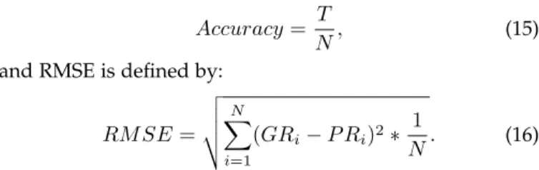
TABLE 1: Statistics of three benchmark datasets Two commonly used performance evaluation metrics are used. The first one is accuracy and the second one is rooted mean square error (RMSE).6LetGR
ibe the golden sentiment rating, P Ri be the predicted sentiment rating, and T be the number of documents where GRi = P Ri. Accuracy is then defined by
Accuracy= T
N, (15)
and RMSE is defined by:
RM SE= v u u t N X i=1 (GRi−P Ri)2∗ 1 N. (16)
Note that RMSE is only suitable for range based labels, Hence, in our paper, RMSE is used only in IMDB, Yelp13, and Yelp14 for evaluation.
We train the skip-gram word embedding [80] on each dataset separately to initialize the word vectors. All embed-ding sizes on the model are set to 200, which is the same as [6], [7], [10], [36].
6. Normally accuracy is a problematic measure in highly unbalanced datasets. But in IMDB, the largest class only takes less than 20% of all instances. The most imbalanced data are Yelp 13 whose largest class is 41% among 5 classes and second largest is about 30%. IMDB has a 50/50 split for 2-classes.
Sentences Tokens Participants Mishra [55] (M) 994 68543 7 Dundee (D) 2,368 51,502 10 GECO (G) 4,934 774,015 17
TABLE 2: General statistics of three eye-tracking corpus
Three sets of experiments are conducted. The first is on the selection of the regression model for reading time prediction. The second set of experiments compares our proposed CGA with another sentiment analysis method which use text only. The third set of experiments evaluates the effectiveness of combining different attention models.
4.1 Reading time prediction
Reading time prediction, using regression models, are trained from eye-tracking data. In this work, we use three sets of public available tracking data. Ideally, an eye-tracking corpus built from on-line reviews is more suitable for our experiments. But, we can only work with what is available. Their lengths in terms sentence and tokens as well as the number of participants are listed inTable 2.
Though our regression models, we learn to predict read-ing time from lexical and context features as discussed in 3.1. We take the first 90% of sentences as training data and the rest 10% as test data. We compare our regression model with more complex deep learning based regression models in each of the three eye-tracking datasets.7
In addition to the linear regression model(LL) and the Ridge regression model(RR), we also choose the Support Vector Machine (SVM) model with linear kernel, the Recur-rent Neural Network (RNN) model and the Long Short Time Memory (LSTM) model for regression learning. For both models, there are two versions. The basic version inputs the extracted feature sets as word representation, labeled as SVM-1, RNN-1 and LSTM-1, respective. The second version takes word embedding (dimension set to 200) [81] as the initial word representation input, labeled as SVM-2, RNN-2 and LSTM-2, respectively. The configuration that performs the best for each model is selected and the performance re-sults are listed in Table 3. Data inTable 3are in milliseconds.
GECO DUNDEE Mishra RR 69.47 70.52 84.22 LR 72.47 73.52 87.25 SVM-1 73.46 77.50 88.96 RNN-1 75.47 83.52 96.23 LSTM-1 79.47 84.52 114.25 SVM-2 78.47 82.52 87.92 RNN-2 79.57 86.47 101.25 LSTM-2 83.88 95.88 122.27
TABLE 3: RMSE for reading time prediction Table 3 shows that Ridge regression gives the best result in all three datasets, and both regression models outperform SVM and deep learning based models. The reason that Ridge regression(RR) has the best performance in all the three datasets is that regularization in RR reduces the over-fitting problem. Results of SVM and deep learning model
7. Mishra et al. [55] only provides fixation time. Fixation time is used when training by this set of eye-tracking data.
with word embedding initialization partly support the fact that reading time are more dependent on micro level syntax and semantic feature of a word, such as number of letters in word and complexity score of the word instead of deep level global context features.
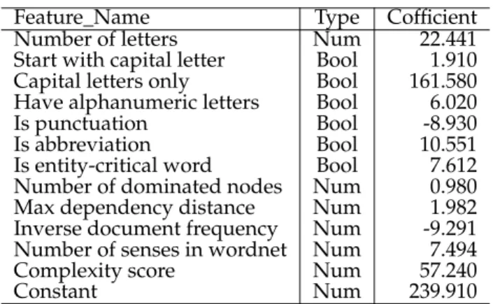
We also use coefficient of determination to describe the relationship between predicted reading time and actual reading time in eye-tracking data. In the three eye-tracking datasets, RR can achieve coefficient of determination8 at 0.32, 0.30 and 0.27 in three eye-tracking datasets. The fea-tures, their types and the corresponding coefficients in RR are shown inTable 4. Again, the features shown inTable 4
are microlevel features.
Feature Name Type Cofficient
Number of letters Num 22.441
Start with capital letter Bool 1.910
Capital letters only Bool 161.580
Have alphanumeric letters Bool 6.020
Is punctuation Bool -8.930
Is abbreviation Bool 10.551
Is entity-critical word Bool 7.612 Number of dominated nodes Num 0.980
Max dependency distance Num 1.982
Inverse document frequency Num -9.291 Number of senses in wordnet Num 7.494
Complexity score Num 57.240
Constant Num 239.910
TABLE 4: Major features used for ridge Regression on Eye-Tracking Data(Num stand for numerical feature and Bool stand for boolean feature)
4.2 Comparison of different sentiment classification
methods
Because the features used in our model are all text based, we compare CGA with three groups of baseline methods which also only use review text for learning. Group 1 methods include commonly known linguistic and context features for SVM classifiers. Group 2 includes recent sentiment classifi-cation algorithms which are top performers using review text for training, without attention mechanisms. Group 3 includes two state-of-the-art attention methods.
• Majority— A simple majority based classifier based on sentence labels.
• Trigram — A SVM classifier using uni-grams/bigrams/trigram as features.
• Text feature — A SVM classifier using word level and context level features, such as n-gram and senti-ment lexicons.
• AvgWordvec— A SVM classifier that takes the aver-age of word embeddings in Word2Vec as document embedding.
Here is a list of Group 2 methods:
• SSWE[82] — A SVM classifier using sentiment spe-cific word embedding.
• RNTN+RNN [26] — A Recursive Neural Tensor Network (RNTN) to represent sentences and trained with RNN model.
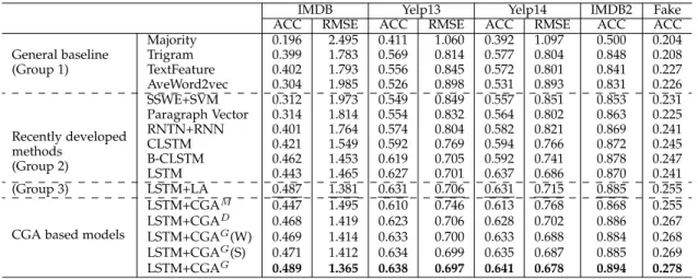
IMDB Yelp13 Yelp14 IMDB2 Fake ACC RMSE ACC RMSE ACC RMSE ACC ACC General baseline (Group 1) Majority 0.196 2.495 0.411 1.060 0.392 1.097 0.500 0.204 Trigram 0.399 1.783 0.569 0.814 0.577 0.804 0.848 0.208 TextFeature 0.402 1.793 0.556 0.845 0.572 0.801 0.841 0.227 AveWord2vec 0.304 1.985 0.526 0.898 0.531 0.893 0.831 0.226 Recently developed methods (Group 2) SSWE+SVM 0.312 1.973 0.549 0.849 0.557 0.851 0.853 0.231 Paragraph Vector 0.314 1.814 0.554 0.832 0.564 0.802 0.863 0.225 RNTN+RNN 0.401 1.764 0.574 0.804 0.582 0.821 0.869 0.241 CLSTM 0.421 1.549 0.592 0.769 0.594 0.766 0.872 0.245 B-CLSTM 0.462 1.453 0.619 0.705 0.592 0.741 0.878 0.247 LSTM 0.443 1.465 0.627 0.701 0.637 0.686 0.870 0.241 (Group 3) LSTM+LA 0.487 1.381 0.631 0.706 0.631 0.715 0.885 0.255 CGA based models
LSTM+CGAM 0.447 1.495 0.610 0.746 0.613 0.768 0.868 0.255
LSTM+CGAD 0.468 1.419 0.623 0.706 0.628 0.702 0.886 0.267
LSTM+CGAG(W) 0.469 1.414 0.633 0.700 0.633 0.688 0.884 0.268
LSTM+CGAG(S) 0.471 1.412 0.634 0.699 0.635 0.687 0.885 0.269
LSTM+CGAG 0.489 1.365 0.638 0.697 0.641 0.678 0.894 0.278 TABLE 5: Evaluation on sentiment classification using only review text for training
• Paragraph vector [83] — A SVM classifier using document embedding as features.
• CLSTM [84] — A Cached LSTM to capture the overall semantic information in long text. The two variations include regularCLSTMand bi-directional
B-CLSTM.
Here is a list of Group 3 methods which use attention mechanism:
• LSTM+LA[7] — State-of-the-art LSTM using local context as attention mechanism in both sentence level and document level.
• LSTM+UPA[7] — A State-of-the-art LSTM including LA as well as user/product as attention mechanism at both sentence level and document level. This method only used when user/product information is available.
Our proposed CGA model has several variations as explained below.
• LSTM+CGA — A LSTM classifier using only CGA model at sentence level and document level. Based on the three eye-tracking datasets (GECO, DUNDEE and Mishra’s) for reading time pre-diction, we label the same model by different training data as LSTM+CGAG,LSTM+CGAD and
LSTM+CGAM (G,D,M represent three different eye-tracking datasets: GECO, DUNDEE and Mishra’s). For LSTM+CGAG, we evaluate the importance of word level attention and sentence level at-tention by using atat-tention mechanism only on word level (LSTM+CGAG(W)) or sentence level (LSTM+CGAG(S)).
• LSTM+CGA+LAG— A LSTM based classifier using both the CGA model and Yang et al.’s [36] local text context based attention model(LA) [7]. Since combining methods can either be serial or in paral-lel, there are actually two corresponding variations: LSTM+CGA+LAGs and LSTM+CGA+LAGp.
• LSTM+CGA+UPAG — The same framework to
LSTM+CGA+LAGwith an additional user/product attention. The user/production attention is built from user and product information for all datasets
except IMDB2. The two corresponding variations are LSTM+CGA+UPAGs and LSTM+CGA+UPA
G p. We split train/development/test set in the rate of 8:1:1. The best configuration of the development dataset is used in the test set to obtain the final result.Table 5shows the performance of the three groups using review text without user/product information. Among all the reference meth-ods that do not use any attention mechanism including all methods in Group 1 and Group 2, LSTM is the best performer. This shows the advantage of using deep learning in recent development. LSTM+LA [7] in Group 3 is the state-of-the-art method which uses local attention mechanism to improve performance significantly compare to all methods in Group 1 and Group2. Among our CGA based varia-tions, using the GECO dataset gives the best result outper-forming LSTM+LA in all three datasets. LSTM+CGAG has significant improvement over LSTM+LA with p values of
p <0.016on IMDB,p <0.0019on Yelp 13,p <0.00023on Yelp 14 ,andp <10−9 on FND. LSTM+CGAG has the best result compared to the other two variations because GECO has larger participant size. Its text genre is also closer to the review datasets for sentiment analysis. This proves that the additional cognition grounded data can boost the attention model to improve the performance of sentiment analysis.
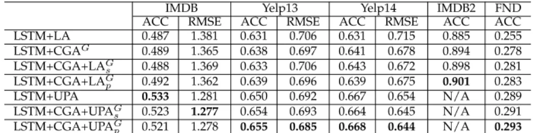
In the third set of experiment, we compare our LSTM+CGA model with the combination of other attention models including the LA model and the UPA model as shown in Table 6. Since the GECO dataset gives the best performance as shown in previous experiments, Results given in Table 6 show the performance of LSTM+CGA using only the GECO dataset. Note that UPA is is an enhanced version of LA based on additional user/product information. So it works only if user/product information is available. Such data is provided in the first three datasets. For the FND dataset, speaker information is used to replace user information, and there is no product information.
Table 6shows that among all three single attention mod-els, UPA outperforms both LA and CGA in the first three datasets. This is easy to understand as UPA already included LA and it has additional information from users and prod-ucts for its attention model. The combined method of CGA with UPA can still further improve performance. When CGA+UPA are combined in parallel, it has the best
perfor-IMDB Yelp13 Yelp14 IMDB2 FND ACC RMSE ACC RMSE ACC RMSE ACC ACC LSTM+LA 0.487 1.381 0.631 0.706 0.631 0.715 0.885 0.255 LSTM+CGAG 0.489 1.365 0.638 0.697 0.641 0.678 0.894 0.278 LSTM+CGA+LAG s 0.488 1.369 0.633 0.706 0.643 0.672 0.898 0.281 LSTM+CGA+LAG p 0.492 1.362 0.639 0.696 0.639 0.675 0.901 0.283 LSTM+UPA 0.533 1.281 0.650 0.692 0.667 0.654 N/A 0.289 LSTM+CGA+UPAG s 0.523 1.277 0.654 0.693 0.664 0.645 N/A 0.291 LSTM+CGA+UPAG p 0.521 1.278 0.655 0.685 0.668 0.644 N/A 0.293 TABLE 6: Evaluation on sentiment classification on using dual attention models
IMDB Yelp13 Yelp14 IMDB2 FND Affective meaning Lexicon type ACC RMSE ACC RMSE ACC RMSE ACC ACC LSTM baseline N/A 0.443 1.465 0.627 0.701 0.637 0.686 0.870 0.241 Sentiment lexicon (Group 1) VADER 0.481 1.371 0.631 0.705 0.624 0.697 0.883 0.259 Sentiwordnet 0.341 1.701 0.607 0.747 0.611 0.733 0.854 0.237 Sentinet 0.372 1.608 0.614 0.733 0.601 0.734 0.851 0.239 VAD(EPA) methods (Group 2) ANEW 0.467 1.362 0.626 0.704 0.626 0.699 0.890 0.260 EPA 0.469 1.369 0.631 0.706 0.627 0.704 0.891 0.259 DAL 0.471 1.376 0.626 0.702 0.631 0.684 0.884 0.258 Others (Group 3) Concreteness 0.458 1.435 0.635 0.684 0.625 0.694 0.886 0.264 Perceptual 0.460 0.374 0.630 0.687 0.624 0.701 0.877 0.257 Eye-tracking Eye-tracking 0.489 1.365 0.638 0.697 0.641 0.678 0.894 0.278
TABLE 7: Compare with other lexicons without using user/product information
mance for Yelp13, Yelp14, and FND (with pvalue of 0.027 ,0.032 and 0.0017 respectively compare to LSTM+UPA). In the IMDB dataset, however, UPA has the best performance. This may be because user/product information is more effective in the movie review IMDB dataset which is more subjective.
Since the UPA model works only if user/product in-formation is available, for IMDB2, which does not have user/product information, only CGA and LA models work and the combined use of CGA+LA gives the best perfor-mance. Experiment indicate that incorporate in different aspects of attention are commendable. As the best result, the CGA model can work with others to take the full advantage of attention models in neural network based sentiment analysis.
4.3 Comparison of attention models based on other
lexicons
Other lexicon-based resources can also serve as knowledge to build attention models. In [85], different lexicons were used to build attention models. Sentiment lexicons can be used directly to build attention modes for sentiment analysis by simply taking the sentiment values as attention weights. In other words, we can build LSMT+CGA withtwireplaced
by sentiment values in a sentiment lexicon. In this third experiment, we compare the use of eye-tracking data with other lexicons used by Li et al. [20]. We divided the lexicons in three groups.
The first group include commonly used sentiment lexi-cons:
• VADER [86] is sentiment lexicons annotated with in-tensity and VADER also contains standard deviation of the annotation process.
• SentiWordNet [87] is a lexical resource for opin-ion mining. SentiWordNet assigns to each synset of WordNet [88] with three sentiment scores: positivity, negativity, objectivity.
• SenticNet [67] [89] provides a set of semantics, syn-taxes, and polarity associated with 50,000 natural language concepts.
The second group includes three multi-dimensional af-fective lexicons In these three afaf-fective lexicons, at least one dimension is directly link to sentiment. Thus, data in that dimension is used to serve as sentiment values.
• ANEW (the affective norms for English) [75] pro-vides a set of normative emotional ratings for a large number of words in the English language. This set of verbal materials have been rated in terms of pleasure, arousal, and dominance to complement the existing International Affective Picture System. The extended version of ANEW lexicon consist of 13,915 words. ANEW based on the Valance-arousal-dominance schema (VAD), The valence dimension can directly serve as sentiment.
• EPA (evaluation, potency, and activity) [90]is anno-tated in the three dimensions of evaluation, potency, and activity. In those three dimension, evaluation is close related to sentiment. Here the evaluation dimension is close to sentiment and it can be used to approximate sentiment.
• DAL (The Dictionary of Affect in Language) [91] is a lexicon annotated in the dimensions of pleasantness-activation-imagery contains 8,742 terms. The Pleas-ant dimension can directly serve as the sentiment dimension.
The third group include two lexicons, one is to measure concreteness of concept terms, and the other is to measure perceptual sense which measures in cognition. They are evaluated to see how cognition linked lexicons can help in sentiment analysis.
• Concreteness [92] is annotated on the degree of con-creteness or abstractness of a word through crowd-sourcing.
IMDB YELP13 YELP14 FND ACC RMSE ACC RMSE ACC RMSE ACC UPA only 0.533 1.281 0.650 0.692 0.667 0.654 0.289 VADER 0.515 1.318 0.647 0.681 0.654 0.678 0.286 SentiwordNet3 0.423 1.501 0.624 0.730 0.647 0.688 0.256 SentiNet4 0.433 1.487 0.620 0.743 0.648 0.667 0.258 ANEW 0.515 1.328 0.648 0.679 0.661 0.671 0.285 EPA 0.514 1.334 0.648 0.675 0.651 0.675 0.286 DAL 0.518 1.328 0.644 0.694 0.663 0.672 0.288 CONCRESNESS 0.518 1.303 0.647 0.681 0.661 0.671 0.285 Perceptual senses 0.515 1.308 0.645 0.683 0.659 0.670 0.283 Eye-tracking 0.521 1.278 0.655 0.685 0.668 0.644 0.293
TABLE 8: Compare with other attention mechanism in dual attention mechanism (with UAP+P)
The shelteron hotel is lucky to receive 2starts from me considering Pun VADER 0.063 0.020 0.079 0.148 0.264 0.146 0.174 0.020 0.097 0.025 0.007 0.000 SentiWordNet3 0.000 0.050 0.000 0.040 0.880 NA 0.040 0.010 0.000 0.010 0.020 0.000 SentiNet4 0.033 0.020 0.039 0.105 0.508 NA 0.061 0.010 0.099 0.133 0.022 0.000 ANEW 0.098 0.010 0.120 0.107 0.133 0.116 0.129 0.010 0.093 0.105 0.100 0.000 EPA 0.033 0.040 0.123 0.120 0.151 0.127 0.158 0.020 0.116 0.114 0.060 0.000 DAL 0.104 0.030 0.128 0.099 0.150 0.094 0.145 0.030 0.084 0.111 0.084 0.000 CONCRETNESS 0.155 0.030 0.204 0.066 0.073 0.064 0.111 0.040 0.076 0.179 0.072 0.000 Perceptual strength 0.105 0.040 0.103 0.104 0.109 0.077 0.107 0.030 0.122 0.138 0.136 0.000 Eye-tracking 0.070 0.086 0.078 0.082 0.078 0.072 0.088 0.116 0.071 0.078 0.082 0.082
TABLE 9: Case study on attention weights of using other lexicons and eye-tracking data
• Perceptual sense [93], [94] is annotated with percep-tual strength of a target word by feeling through five sensations (touch, hearing, seeing, smelling ,and tasting).
Table 7 shows the comparison in the situation that user/product situation is not available. We can observed that nearly all sentiment lexicon except SentiWordnet and SentNet can outperform regular LSTM in four datasets. But all lexicons do not match the performance of LA and CGA models. InTable 8, we evaluate attention models based on these lexicons by perform dual attention mechanism with user/product attention.Table 8shows similar performance result which shows that using lexicon resources alone do not match up with LA based and CGA methods. The likely reason for this is that the sentiment values of each word in these lexicons are context-independent. That is, their values are fixed in the lexicon relative only to different entries in the same lexicons. On the other hand, the attention weight of each word in a sentence should be context-related. In other words, the attention weights of certainly words should be relative to other words in the same sentence (and/or documents) which is how they are produced in both LA based and CGA based methods. This is the main reason to explain the underperformance of lexicon based methods.
4.4 Case study
A random sentence sample ’The Shelton hotel is lucky to receive 2stars from me considering ...’ is taken from Yelp13 dataset to demonstrate the difference in the three attention mechanisms, i.e. local text (LA), cognition-based (CGA), and user/product attention(UPA). Figure 1 shows visually the difference in attention weights of the three models.
The attention weights of words in the LA model does not change much. CGA, on the other hand, gives higher weights to the sentiment linked word2starsand the verbreceive. This two words do play significant roles as an indirect object and a main verb, respectively. This case shows that CGA
Fig. 1: Case Study on attention weights in three different attention mechanisms
does a better job in capturing micro level information in the sentence level. This support the experimental results in
Table 5andTable 6.
Table 9 compares our CGA with attention models based on other lexicons. We can observe that Sentiword-net and SentiSentiword-net give the sentiment word ”lucky” a very heavy weight while another words received relative low weight.This partly explains why these two lexicon achieves lowest performances in all lexicons. VADER, EPA and DAL give relative high weight to notional words. But they assign very low weight to functional words. This result indicates that the effect of function words should not be under esti-mated.
For Group 3 lexicons concreteness and perceptual are not in sentiment space. But they still encode some valid seman-tic information as useful knowledge. For concreteness value, the subject of sentence ”hotel” receives the highest weight
in all words. But in eye-tracking data and user/product attention, ”hotel” does not have a particular heavy weight.
5
CONCLUSION
In this paper, we propose a novel cognition grounded atten-tion model to improve the state-of-the-art neural sentiment analysis model through cognition grounded eye-tracking data. A simple and effective regression model is used to predict reading time using both eye-tracking data and local text features. The predicted reading time is then used to build an attention layer in neural sentiment analysis mod-els. The attention model considers both reading time and other syntactic and context features. The CGA model also considers both sentence level context and document context. Evaluation on benchmark datasets validates the effec-tiveness of our method in sentiment analysis and related tasks as our method clearly outperforms other state-of-the-art methods that use local context information to build their attention models. The CGA mechanism can also be combined with other attention mechanisms to provide room for further improvement. We compare the eye-tracking data with other lexical resources including sentiment lexicons, dimension based affective lexicons, and other cognition based resources.
One important reason that our CGA model prevails over other lexicons is that CGA can extract context relevant infor-mation including both sentence level context and document level context.
An important finding of our work is that cognition grounded data gives better gain in attention models to improve the performance of sentiment analysis. Our work also indicates that both the quality and the scale of eye-tracking data have great influence on the effectiveness of the CGA model. We anticipate even greater improvement with a larger scale eye-tracking data in similar genre as the sentiment analysis text.
ACKNOWLEDGMENT
The work is partially supported by the research grants from Hong Kong Polytechnic University (PolyU RTVU) and GRF grant (CERG PolyU 15211/14E, PolyU 152006/16E).
Yunfei Long acknowledges the financial support of the NIHR Nottingham Biomedical Research Centre and NIHR MindTech Healthcare Technology Co-operative.
REFERENCES
[1] R. Dong, M. P. O’Mahony, M. Schaal, K. McCarthy, and B. Smyth, “Sentimental product recommendation,” inProceedings of the 7th ACM conference on Recommender systems, pp. 411–414, ACM, 2013. [2] B. Pang, L. Lee,et al., “Opinion mining and sentiment analysis,”
Foundations and TrendsR in Information Retrieval, vol. 2, no. 1–2, pp. 1–135, 2008.
[3] C. Clavel and Z. Callejas, “Sentiment analysis: from opinion mining to human-agent interaction,”IEEE Transactions on affective computing, vol. 7, no. 1, pp. 74–93, 2016.
[4] B. Pang, L. Lee, and S. Vaithyanathan, “Thumbs up?: sentiment classification using machine learning techniques,” inProceedings of the ACL-02 conference on Empirical methods in natural language processing-Volume 10, pp. 79–86, Association for Computational Linguistics, 2002.
[5] A. Vanzo, D. Croce, and R. Basili, “A context-based model for sentiment analysis in twitter.,” inCOLING, pp. 2345–2354, 2014.
[6] D. Tang, B. Qin, and T. Liu, “Document modeling with gated re-current neural network for sentiment classification,” inProceedings of the 2015 Conference on Empirical Methods in Natural Language Processing, pp. 1422–1432, 2015.
[7] H. Chen, M. Sun, C. Tu, Y. Lin, and Z. Liu, “Neural sentiment classification with user and product attention,” inProceedings of the 2016 Conference on Empirical Methods in Natural Language Processing, pp. 1650–1659, 2016.
[8] A. L. Maas, R. E. Daly, P. T. Pham, D. Huang, A. Y. Ng, and C. Potts, “Learning word vectors for sentiment analysis,” in Proceedings of the 49th Annual Meeting of the Association for Computational Linguistics: Human Language Technologies-Volume 1, pp. 142–150, Association for Computational Linguistics, 2011.
[9] C. J. Hutto and E. Gilbert, “VADER: A parsimonious rule-based model for sentiment analysis of social media text,” inProceedings of the Eighth International Conference on Weblogs and Social Media (ICWSM), 2014.
[10] D. Tang, B. Qin, and T. Liu, “Learning semantic representations of users and products for document level sentiment classification,” inProc. ACL, 2015.
[11] S. Davis and P. Mermelstein, “Comparison of parametric rep-resentations for monosyllabic word recognition in continuously spoken sentences,”IEEE transactions on acoustics, speech, and signal processing, vol. 28, no. 4, pp. 357–366, 1980.
[12] V. Demberg and F. Keller, “Data from eye-tracking corpora as ev-idence for theories of syntactic processing complexity,”Cognition, vol. 109, no. 2, pp. 193–210, 2008.
[13] L. Gui, R. Xu, Y. He, Q. Lu, and Z. Wei, “Intersubjectivity and senti-ment: from language to knowledge,” inProceedings of International Joint Conference on Artificial Intelligence, pp. 2789–2795, 2016. [14] C. Zhou, J. Bai, J. Song, X. Liu, Z. Zhao, X. Chen, and J. Gao,
“Atrank: An attention-based user behavior modeling framework for recommendation,” inThirty-Second AAAI Conference on Artifi-cial Intelligence, 2018.
[15] Z. Li, Y. Wei, Y. Zhang, and Q. Yang, “Hierarchical attention transfer network for cross-domain sentiment classification,” in
Proceedings of the Thirty-Second AAAI Conference on Artificial Intelli-gence, AAAI 2018, New Orleans, Lousiana, USA, February 2–7, 2018, 2018.
[16] S. A. Crossley, K. Kyle, and D. S. McNamara, “Sentiment analysis and social cognition engine (seance): An automatic tool for senti-ment, social cognition, and social-order analysis,”Behavior research methods, vol. 49, no. 3, pp. 803–821, 2017.
[17] I. J. Roseman, “A model of appraisal in the emotion system,”
Appraisal processes in emotion: Theory, methods, research, pp. 68–91, 2001.
[18] M. Barrett, J. Bingel, F. Keller, and A. Søgaard, “Weakly supervised part-of-speech tagging using eye-tracking data,” in Proceedings of the 54th Annual Meeting of the Association for Computational Linguistics (Volume 2: Short Papers), vol. 2, pp. 579–584, 2016. [19] K. Rayner, “Eye movements in reading and information
process-ing: 20 years of research.,” Psychological bulletin, vol. 124, no. 3, p. 372, 1998.
[20] M. Li, Q. Lu, Y. Long, and L. Gui, “Inferring affective meanings of words from word embedding,”IEEE Transactions on Affective Computing, 2017.
[21] S. Kolkur, G. Dantal, and R. Mahe, “Study of different levels for sentiment analysis,”International Journal of Current Engineering and Technology, vol. 5, no. 2, pp. 768–770, 2015.
[22] M. Pontiki, D. Galanis, H. Papageorgiou, I. Androutsopoulos, S. Manandhar, M. AL-Smadi, M. Al-Ayyoub, Y. Zhao, B. Qin, O. De Clercq,et al., “Semeval-2016 task 5: Aspect based sentiment analysis,” in ProWorkshop on Semantic Evaluation (SemEval-2016), pp. 19–30, Association for Computational Linguistics, 2016. [23] K. McKeown, D. Jordan, and V. Hatzivassiloglou, “Generating
patient-specific summaries of online literature,” inProc. of Intel-ligent Text Summarization, AAAI Spring Symposium, Citeseer, 1998. [24] R. Xia, C. Zong, and S. Li, “Ensemble of feature sets and
classifica-tion algorithms for sentiment classificaclassifica-tion,”Information Sciences, vol. 181, no. 6, pp. 1138–1152, 2011.
[25] R. Socher, J. Pennington, E. H. Huang, A. Y. Ng, and C. D. Man-ning, “Semi-supervised recursive autoencoders for predicting sen-timent distributions,” inProceedings of the Conference on Empirical Methods in Natural Language Processing, pp. 151–161, Association for Computational Linguistics, 2011.
[26] R. Socher, A. Perelygin, J. Y. Wu, J. Chuang, C. D. Manning, A. Y. Ng, and C. Potts, “Recursive deep models for semantic
compositionality over a sentiment treebank,” in Proceedings of the conference on empirical methods in natural language processing (EMNLP), vol. 1631, p. 1642, Citeseer, 2013.
[27] O. Irsoy and C. Cardie, “Opinion mining with deep recurrent neural networks.,” inEMNLP, pp. 720–728, 2014.
[28] Y. Bengio, P. Simard, and P. Frasconi, “Learning long-term depen-dencies with gradient descent is difficult,”IEEE transactions on neural networks, vol. 5, no. 2, pp. 157–166, 1994.
[29] D. Tang, B. Qin, and T. Liu, “Learning semantic representations of users and products for document level sentiment classification,” in Proceedings of the 53rd Annual Meeting of the Association for Computational Linguistics and the 7th International Joint Conference on Natural Language Processing (Volume 1: Long Papers), (Beijing, China), pp. 1014–1023, Association for Computational Linguistics, July 2015.
[30] J. Weston, S. Chopra, and A. Bordes, “Memory networks,” in
Proceedings of the 6th International Conference on Learning Represen-tations, pp. 1–15, ACM, 2015.
[31] S. Sukhbaatar, J. Weston, R. Fergus, and others, “End-to-end mem-ory networks,” inAdvances in neural information processing systems, pp. 2440–2448, 2015.
[32] Z.-Y. Dou, “Capturing user and product information for docu-ment level sentidocu-ment analysis with deep memory network,” in
Proceedings of the 2017 Conference on Empirical Methods in Natural Language Processing, pp. 521–526, Association for Computational Linguistics, 2017.
[33] Y. Long, M. Ma, Q. Lu, R. Xiang, and C.-R. Huang, “Dual memory network model for biased product review classification,” in Proceedings of the 9th Workshop on Computational Approaches to Subjectivity, Sentiment and Social Media Analysis, pp. 140–148, 2018. [34] D. Tang, B. Qin, and T. Liu, “Aspect level sentiment classification with deep memory network,” inProceedings of the 2016 Conference on Empirical Methods in Natural Language Processing, pp. 214–224, Association for Computational Linguistics, 2016.
[35] M. H. F. Keller, “Modeling human reading with neural attention,” in Proceedings of the Conference on Empirical Methods in Natural Language Processing, pp. 85–95, 2016.
[36] Z. Yang, D. Yang, C. Dyer, X. He, A. Smola, and E. Hovy, “Hierarchical attention networks for document classification,” in
Proceedings of the 2016 Conference of the North American Chapter of the Association for Computational Linguistics: Human Language Technologies, 2016.
[37] A. Zadeh, P. P. Liang, S. Poria, P. Vij, E. Cambria, and L.-P. Morency, “Multi-attention recurrent network for human communication comprehension,” in Thirty-Second AAAI Conference on Artificial Intelligence, 2018.
[38] S. Mohammad, S. Kiritchenko, P. Sobhani, X. Zhu, and C. Cherry, “Semeval-2016 task 6: Detecting stance in tweets,” inProceedings of the 10th International Workshop on Semantic Evaluation (SemEval-2016), pp. 31–41, 2016.
[39] R. X. M. L. Yunfei Long, Qin Lu and C. ren Huang, “Fake news detection through multi-perspective speaker profiles,” in
Proceedings of the 8th International Joint Conference on Natural Lan-guage Processing of the AFNLP: Volume 2-Volume 2, pp. 1039–1047, Association for Computational Linguistics, 2017.
[40] L. Dong, F. Wei, S. Liu, M. Zhou, and K. Xu, “A statistical parsing framework for sentiment classification,”Computational Linguistics, 2015.
[41] D. Yogatama, M. Faruqui, C. Dyer, and N. Smith, “Learning word representations with hierarchical sparse coding,” inProceedings of the 32nd International Conference on Machine Learning (ICML-15), pp. 87–96, 2015.
[42] L. Jacob, G. Obozinski, and J.-P. Vert, “Group lasso with overlap and graph lasso,” in Proceedings of the 26th annual international conference on machine learning, pp. 433–440, ACM, 2009.
[43] Q. Qian, M. Huang, and X. Zhu, “Linguistically regularized lstms for sentiment classification,”Proceedings of the 55th Annual Meeting of the Association for Computational Linguistics, 2016.
[44] A. Mishra, K. Dey, and P. Bhattacharyya, “Learning cognitive fea-tures from gaze data for sentiment and sarcasm classification using convolutional neural network,” inProceedings of the 55th Annual Meeting of the Association for Computational Linguistics (Volume 1: Long Papers), vol. 1, pp. 377–387, 2017.
[45] A. Mishra and P. Bhattacharyya, “Predicting readers sarcasm un-derstandability by modeling gaze behavior,” inCognitively Inspired Natural Language Processing, pp. 99–115, Springer, 2018.
[46] A. Mishra, S. Tamilselvam, R. Dasgupta, S. Nagar, and K. Dey, “Cognition-cognizant sentiment analysis with multitask subjectiv-ity summarization based on annotators’ gaze behavior,” in Thirty-Second AAAI Conference on Artificial Intelligence, 2018.
[47] T. Blascheck, K. Kurzhals, M. Raschke, M. Burch, D. Weiskopf, and T. Ertl, “State-of-the-art of visualization for eye tracking data,” in
Proceedings of EuroVis, vol. 2014, 2014.
[48] A. Joshi, A. Mishra, N. Senthamilselvan, and P. Bhattacharyya, “Measuring sentiment annotation complexity of text.,” inACL (2), pp. 36–41, 2014.
[49] A. Mishra, A. Joshi, and P. Bhattacharyya, “A cognitive study of subjectivity extraction in sentiment annotation,”ACL 2014, p. 142, 2014.
[50] A. Mishra, D. Kanojia, S. Nagar, K. Dey, and P. Bhattacharyya, “Leveraging cognitive features for sentiment analysis,” CoNLL 2016, p. 156, 2016.
[51] S. Joshi, D. Kanojia, and P. Bhattacharyya, “More than meets the eye: Study of human cognition in sense annotation.,” in HLT-NAACL, pp. 733–738, 2013.
[52] A. Mishra, P. Bhattacharyya, M. Carl, and I. CRITT, “Automatically predicting sentence translation difficulty.,” inACL (2), pp. 346–351, 2013.
[53] A. Kennedy, “The dundee corpus [cd-rom],” Psychology Depart-ment, University of Dundee, 2003.
[54] U. Cop, N. Dirix, D. Drieghe, and W. Duyck, “Presenting geco: An eyetracking corpus of monolingual and bilingual sentence reading,”Behavior research methods, pp. 1–14, 2016.
[55] A. Mishra, D. Kanojia, and P. Bhattacharyya, “Predicting readers’ sarcasm understandability by modeling gaze behavior.,” inAAAI, pp. 3747–3753, 2016.
[56] K. Tomanek, U. Hahn, S. Lohmann, and J. Ziegler, “A cognitive cost model of annotations based on eye-tracking data,” in Proceed-ings of the 48th Annual Meeting of the Association for Computational Linguistics, pp. 1158–1167, Association for Computational Linguis-tics, 2010.
[57] P. J. Stone, D. C. Dunphy, M. S. Smith, and D. M. Ogilvie, “The General Inquirer: A Computer Approach to Content Analysis.,”
Journal of Regional Science, vol. 8, no. 1, pp. 113–116, 1968. [58] T. Wilson, J. Wiebe, and P. Hoffmann, “Recognizing Contextual
Polarity in Phrase-Level Sentiment Analysis,” in Proceedings of Human Language Technology Conference and Conference on Empirical Methods in Natural Language Processing, pp. 347–354, 2005. [59] S. M. Mohammad, S. Kiritchenko, and X. Zhu, “NRC-Canada:
Building the state-of-the-art in sentiment analysis of tweets,” in
Proceedings of the 7th International Workshop on Semantic Evaluation, SemEval@NAACL-HLT, pp. 321–327, 2013.
[60] S. Rosenthal, P. Nakov, S. Kiritchenko, S. M. Mohammad, A. Ritter, and V. Stoyanov, “Semeval-2015 task 10: Sentiment analysis in twitter,” inProceedings of the 9th International Workshop on Semantic Evaluation, SemEval@NAACL-HLT 2015, pp. 451–463, 2015. [61] M. M. Bradley and P. J. Lang, “Affective norms for English words
(ANEW): Instruction manual and affective ratings,” tech. rep., Technical report C-1, the center for research in psychophysiology, University of Florida, 1999.
[62] L.-C. Yu, L.-H. Lee, S. Hao, J. Wang, Y. He, J. Hu, K. R. Lai, and X. Zhang, “Building Chinese Affective Resources in Valence-Arousal Dimensions,” inProceedings of the Conference of the North American Chapter of the Association for Computational Linguistics: Human Language Technologies (NAACL-HLT), pp. 540–545, 2016. [63] C. Whissell, “The dictionary of affect in language,”Emotion:
The-ory, research, and experience, vol. 4, no. 113-131, p. 94, 1989. [64] D. R. Heise, “Affect control theory: Concepts and model,” The
Journal of Mathematical Sociology, vol. 13, no. 1-2, pp. 1–33, 1987. [65] D. S. Schmidtke, T. Schrder, A. M. Jacobs, and M. Conrad,
“ANGST: Affective norms for German sentiment terms, derived from the affective norms for English words,” Behavior Research Methods, vol. 46, pp. 1108–1118, Jan. 2014.
[66] B. Liu, “Sentiment analysis and opinion mining,”Synthesis Lectures on Human Language Technologies, vol. 5, no. 1, pp. 1–167, 2012. [67] E. Cambria, S. Poria, R. Bajpai, and B. Schuller, “SenticNet 4:
A semantic resource for sentiment analysis based on conceptual primitives,” inPreceedings of the 26th International Conference on Computational Linguistics (COLING), (Osaka, Japan), pp. 2666–2677, 2016.
[68] W. L. Hamilton, K. Clark, J. Leskovec, and D. Jurafsky, “Inducing Domain-Specific Sentiment Lexicons from Unlabeled Corpora,” in