ISTANBUL TECHNICAL UNIVERSITY GRADUATE SCHOOL OF SCIENCE ENGINEERING AND TECHNOLOGY
M.Sc. THESIS
MAY 2015
ULTRASOUND IMAGE SEGMENTATION USING THE WATERSHED ALGORITHM
Sibel KADIOĞLU
Department of Electronics and Communication Engineering Telecommunication Engineering Programme
SINIRLAMA METODU KULLANARAK ULTRASON GÖRÜNTÜSÜ BÖLÜTLEME
ÖZET
Ultrason görüntülemesi tıp alanında yaygın olarak kullanılan bir görüntüleme tekniğidir. Bu teknik, herhangi bir yan etkisinin olmamasına, hareketli organların gerçek zamanda izlenebilmesine olanak sağlaması ve invazif olmaması özelliklerinden dolayı tıbbi amaçlı görüntülemede oldukça önemli bir yer tutmaktadır. Bilgisayar destekli yöntemler hem ultrason görüntülerinin kalitesinin
MAY 2015
ISTANBUL TECHNICAL UNIVERSITY GRADUATE SCHOOL OF SCIENCE ENGINEERING AND TECHNOLOGY
ULTRASOUND IMAGE SEGMENTATION USING THE WATERSHED ALGORITHM
M.Sc. THESIS Sibel KADIOĞLU
(504121331)
Department of Electronics and Communication Engineering Telecommunication Engineering Programme
Anabilim Dalı : Herhangi Mühendislik, Bilim Programı : Herhangi Program
MAYIS 2015
İSTANBUL TEKNİK ÜNİVERSİTESİ FEN BİLİMLERİ ENSTİTÜSÜ
ULTRASON GÖRÜNTÜLERİNİN HAVZA SINIRLAMA YÖNTEMİ KULLANILARAK BÖLÜTLENMESİ
YÜKSEK LİSANS TEZİ Sibel KADIOĞLU
(504121331)
Elektronik ve Haberleşme Mühendisliği Anabilim Dalı Telekomünikasyon Mühendisliği Programı
Anabilim Dalı : Herhangi Mühendislik, Bilim Programı : Herhangi Program
v
Thesis Advisor : Prof. Dr. Mustafa KARAMAN ... İstanbul Technical University
Jury Members : Prof. Dr. Nizamettin AYDIN ... Yıldız Technical University
Assoc. Prof. Dr. Ender Mete EKŞİOĞLU ... İstanbul Technical University
Sibel Kadıoğlu, a M.Sc. student of ITU Graduate School of Electronics and Communication Engineering Department student ID 504121331, successfully defended the thesis entitled “ULTRASOUND IMAGE SEGMENTATION USING THE WATERSHED ALGORITHM”, which she prepared after fulfilling the requirements specified in the associated legislations, before the jury whose signatures are below.
Date of Submission : 4 May 2015 Date of Defense : 28 May 2015
vii
In loving memory of my father, Necdet Kadıoğlu.
ix FOREWORD
I would like to wholeheartedly thank my advisor Prof. Dr. Mustafa Karaman for his support, guidance, and patience. He not only introduced me to the field of medical image segmentation but also I learnt immensely from his style and work ethics. I would also like to thank Asst. Prof. Dr. Bülent Bolat and Dr. Jouni Pohjalainen for brainstorming on the subject and my family and friends for their support.
xi TABLE OF CONTENTS Page FOREWORD ... ix TABLE OF CONTENTS ... xi ABBREVIATIONS ... xiii LIST OF TABLES ... xv
LIST OF FIGURES ... xvii
SUMMARY ... xix ÖZET ... xxi 1. INTRODUCTION ... 1 1.1 Purpose of Thesis ... 1 1.2 Literature Review ... 2 2. WHAT IS ULTRASOUND? ... 7 2.1 Properties of Ultrasound ... 7 2.2 Ultrasound Imaging ... 8
2.2.1 Ultrasound – tissue interaction ... 10
2.2.2 Ultrasound modes ... 12
3. PREPROCESSING OF ULTRASOUND IMAGES ... 13
3.1 Speckle Noise ... 13
3.2 Speckle Reduction Methods ... 15
3.3 Preprocessing – I: Histogram Equalization ... 16
3.4 Preprocessing – II: Filtering Methods ... 17
3.4.1 Median filter ... 17
3.4.2 Weighted median filter ... 18
3.4.3 Hybrid median filter ... 19
3.4.4 Adaptive median filter ... 20
4. THE WATERSHED ALGORITHM ... 23
4.1 An Overview of Watershed Algorithms ... 23
4.2 Definitions ... 25
4.3 The Vincent – Soille Algorithm ... 27
4.4 The Implementation of the Vincent – Soille Algorithm ... 28
5. POSTPROCESSING OF ULTRASOUND IMAGES ... 31
5.1 Extracting the Regions ... 31
5.2 The Region Merging Algorithm ... 32
5.3 Region Merging based on Size ... 33
5.4 Region Merging based on Intensity ... 34
5.5 Region Merging based on Local Statistics ... 34
6. TEST RESULTS ... 37
6.1 The Ultrasound Test Images ... 38
6.2 The Results of the Watershed Algorithm ... 39
6.2.1 The watershed algorithm on the original images ... 39
xii
6.2.3 The watershed algorithm on local statistics... 43
6.3 The Results of the Region Merging Algorithm ... 45
6.3.1 Parameter selection for region merging ... 45
6.3.2 Region merging based on size on the preprocessed images ... 47
6.3.3 Region merging based on size on the local statistics ... 48
6.3.4 Region merging based on intensity on the preprocessed images ... 49
6.3.5 Region merging based on the local statistics on the preprocessed images 50 7. CONCLUSIONS... 53
8. FUTURE WORK ... 57
REFERENCES ... 59
xiii ABBREVIATIONS
dB : Decibel
PSF : Point Spread Function PSNR : Peak Signal-to-Noise Ratio RAG : Region Adjacency Graph
RF : Radio Frequency
RM : Region Merging
SKIZ : Skeleton Influence Zone SNR : Signal-to-Noise Ratio
US : Ultrasound
WM : Weighted Median
xv LIST OF TABLES
Page Table 6.1 : Statistics on the number of pixels in regions ... 45
xvii LIST OF FIGURES
Page
Figure 1.1 :The overall structure of the work presented in this thesis ... 2
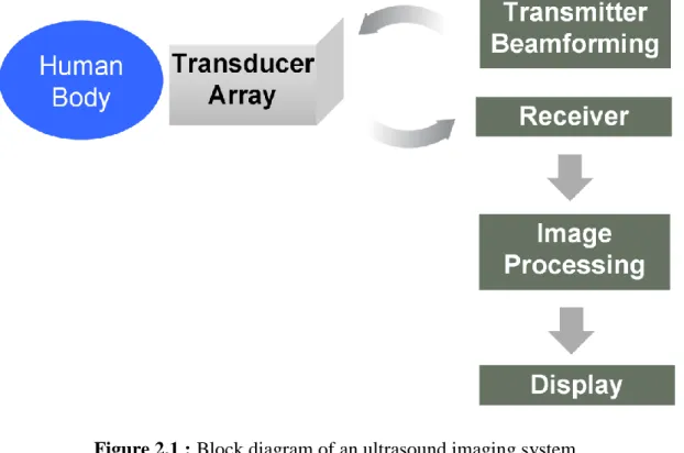
Figure 2.1 : Block diagram of the ultrasound imaging system... 8
Figure 2.2 : Transducer types ... 10
Figure 3.1 : Illustration for computation of hybrid median filter ... 20
Figure 3.2 : Level – I of adaptive median filter. ... 21
Figure 3.3 : Level – II of adaptive median filter. ... 21
Figure 4.1 : Illustration for the immersion-based watershed algorithm ... 27
Figure 5.1 : The general outline of the region merging procedure. ... 32
Figure 6.1 : The overall structure of the algorithms used in this thesis . ... 37
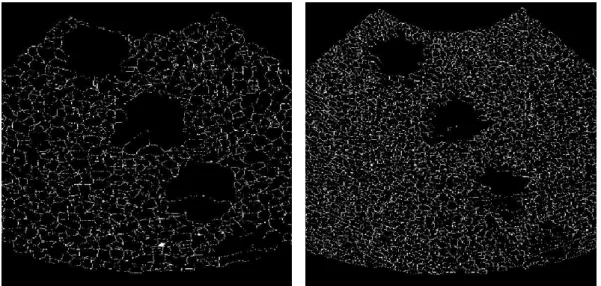
Figure 6.2 : (Left) Cyst phantom image and (Right) Clinical liver image... 39
Figure 6.3 : The result of the watershed algorithm without preprocessing methods on (left) the cyst and (right) the liver images on the original image. ... 40
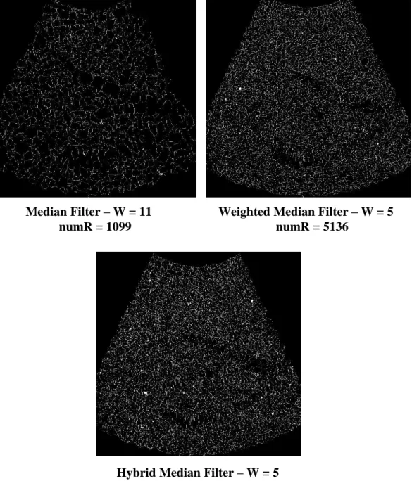
Figure 6.4 : The results of the watershed algorithm on the preprocessed cyst image using different filtering algorithms and window sizes. . ... 41
Figure 6.5 : The results of the watershed algorithm on the preprocessed liver image using different filtering algorithms and window sizes. ... 42
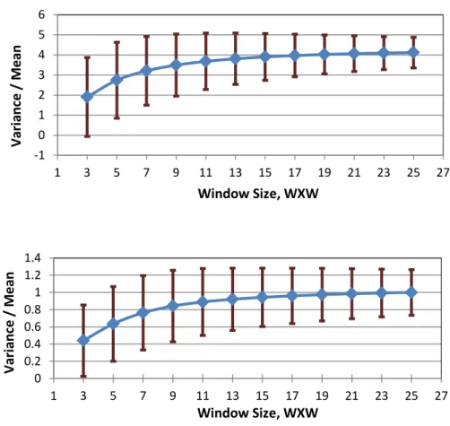
Figure 6.6 : The local statistics computed on different windows for (top) the cyst and (bottom) the liver images. ... 43
Figure 6.7 : The watershed algorithm on the local statistics (top) the cyst and (bottom) the liver images ... 44
Figure 6.8 : The results of the region merging on intensity values based on size criterion (top) the cyst and (bottom) the liver images ... 48
Figure 6.9 : The results of the region merging on alpha values based on size criterion (top) the cyst and (bottom) the liver images ... 49
Figure 6.10 :The results of the region merging on intensity values based on intensity criterion (top) the cyst and (bottom) the liver images. ... 50
Figure 6.11 :The results of the region merging on intensity values based on local statistics criterion (top) the cyst and (bottom) the liver images ... 51
Figure 7.1 :The best resultant images with pre- and postprocessing (top) the cyst and (bottom) the liver images. ... 55
xix
ULTRASOUND IMAGE SEGMENTATION USING THE WATERSHED ALGORITHM
SUMMARY
Ultrasound imaging is an important medical application as it is a safe, non-invasive, and interactive procedure for creating detailed visualization of various structures within the body. Computational methods help improving the quality of ultrasound images as well as they aid in the discovery of important structures. In this line of research, this thesis studies the segmentation problem in general, which aims to identify regions of interest of a given image, and in particular, focuses on its application on ultrasound images using the watershed algorithm.
The thesis consists of three main parts: (i) preprocessing of the ultrasound images, (ii) the watershed algorithm, and (iii) postprocesssing the segmented images.
Despite the technical advances in the clinical field, speckle noise continues to pose a challenge in the interpretation of ultrasound images. The first part of the thesis addresses this issue using preprocessing algorithms, namely; histogram equalization and median-based filters to reduce the speckle noise. This yields an initial improvement in the ultrasound image quality.
Next, in the second part, the watershed algorithm is used on the filtered images to discover important regions. The algorithm works based on an analogy from geography where watershed lines separate catchment basins from each other, hence creating different segments. The algorithm is applied on both intensity values and local statistics which are based on mean and variance values.
A well-known drawback of the watershed algorithm however is that it leads to oversegmentation. Therefore, in the third part, region merging algorithms are studied to overcome this issue. A novel region merging algorithm that incorporates several criteria is proposed. The criteria include the size (the number of pixels in a region), intensity (color values associated with each pixel) and statistical measures (such as variance and mean ratio). These algorithms include three parameters denoted as
Tsize, Tincrement and Tmerge which are image dependent.
Extensive tests run on a phantom cyst image and a clinical liver image. Our test results show that the numbers of regions for the cyst and liver images are reduced by about ~40 and ~50 times, respectively. Overall, we achieved a significant reduction in oversegmentation using a mixture of pre- and postprocessing. The results demonstrate the effects of each studied component; median-based filtering, watershed segmentation, and region merging.
xxi
ULTRASON GÖRÜNTÜLERİNİN HAVZA SINIRLAMA YÖNTEMİ KULLANILARAK BÖLÜTLENMESİ
ÖZET
Ultrason görüntülemesi tıp alanında yaygın olarak kullanılan bir görüntüleme tekniğidir. Bu teknik, herhangi bir yan etkisinin olmamasına, hareketli organların gerçek zamanda izlenebilmesine olanak sağlaması ve invazif olmaması özelliklerinden dolayı tıbbi amaçlı görüntülemede oldukça önemli bir yer tutmaktadır. Bilgisayar destekli yöntemler hem ultrason görüntülerinin kalitesinin artmasına, hem de önemli bölgelerin bulunmasına yardımcı olmaktadır. İş bu tezde, genel olarak, görüntü bölütleme, yani görüntü içerisindeki farklı bölgelerin çıkarılması problemi üzerinde çalışılmakta, özel olarak ise, havza sınırlama metodu kullanılarak, ultrason görüntülerinin bölütlenmesi amaçlanmıştır.
Tez çalışmasının içeriği üç ana bölümden oluşmaktadır: (i) ultrason görüntülerinde ön işleme, (ii) havza sınırlama metodu, (iii) bölütleme sonrası işlemleri.
Klinik alanındaki teknik gelişmelere rağmen, ultrason görüntülerinde meydana gelen benekli yapılar, görüntülerinin yorumlanmasını güçleştirmektedir. Bu nedenle tezin ilk bölümünde bu beneklerin azaltılması amacıyla ön işlemler uygulanmaktadır. Bu ön işlemler, histogram eşitlemesi ve çeşitli medyan filtreleme teknikleridir. Ön işleme metotları ile ultrason görüntülerinde ilk iyileştirmenin yapılması hedeflenmiştir.
Bir sonraki adımda filtrelenmiş görüntüler üzerinde önemli bölgeleri keşfetmek için bölütleme amacıyla havza sınırlama metodu kullanılmaktadır. Bu metot coğrafi yöntemlerden esinlenilmiş olup, havza alanlarını birbirinden ayırarak farklı bölgeler oluşturma prensibine dayanmaktadır. Yöntem, görüntünün gri seviye değerleri ve bu değerlerden elde edilen lokal istatistik değerleri yani ortalama ve değişinti değerleri üzerinde uygulanmaktadır.
Havza bölütleme metodu, aşırı bölütleme ile sonuçlanmaktadır. Bu sebeple, çalışmanın üçüncü bölümünde aşırı bölütleme probleminin çözümü üzerinde durulmaktadır. Bu amaçla farklı kriterleri değerlendirerek çalışan, özgün bir bölge birleştirme metodu geliştirilmiştir. Kriter olarak bölgelerin büyüklüğü (bölge içindeki piksel sayısı), gri seviye değerleri (her piksele karşılık gelen renk değerleri) ve lokal istatistiksel özellikler (değişinti ve ortalama değerleri) baz alınmaktadır.
Bu yöntemler, fantom kist görüntüsü ve klinik karaciğer görüntüsü üzerinde geniş çaplı testler ile denenmiştir. Test sonuçları, kist görüntüsü için bölge sayısının ~40 kat azaltıldığını, karaciger görüntüsü için ise bölge sayısının ~50 kat azaltıldığını göstermektedir. Sonuç olarak, ön ve son işlemler birlikte kullanılarak, aşırı bölütleme probleminin büyük ölçüde azaltılması başarılmıştır. Bu testler, histogram eşitleme, medyan filtre (ve/veya) çeşitleri, havza sınırlama ve bölge birleştirme metodlarının etkisini göstermektedir.
1 INTRODUCTION
1.
Conceptually, segmentation can be described as partitioning of an image into regions that have similar characteristics such as gray level, texture, statistics, and color [1]. Segmentation is used in many applications such as detection, recognition, identification, and image analysis. In medical imaging, image segmentation helps for various objectives including visualization, volumetric measurement, identification of regions of interests (e.g., locating abnormalities), computer integrated surgery, and treatment planning [2].
This thesis focuses on medical image segmentation, and in particular, considers ultrasound images. Ultrasound offers many medical benefits, as it is non-invasive and provides a painless modality that is not harmful for the patient. It performs interactive visualization in real-time, can analyze moving structures and does not include side effects such as radiation. Moreover, ultrasound machines cost less than other imaging methods [3]. As such, ultrasound imaging has great practical importance, and this is our main motivation to study segmentation of ultrasound images. Section 2 provides more information on ultrasound images.
Ultrasound image segmentation is challenging due to several reasons. The main difficulty behind the ultrasound image segmentation is the presence of speckle noise, artifacts, and shadowing [4]. Other challenges include the low level of contrast, namely closeness in gray levels of different tissues as well as the complexity and variability of human body. There are many proposed algorithms to reduce speckle noise and increase image quality, as reviewed in preprocessing methods in Section 3. 1.1Purpose of Thesis
This thesis focuses on ultrasound image segmentation and it is aimed at, first, improving the quality of ultrasound images, and then, identifying important structures in it.
2
Our first goal is to suppress the speckle noise as it negatively affects the segmentation. In Section 3, speckle noise and its properties are described and speckle reduction methods in literature are reviewed. In this thesis, for the purpose of preprocessing, histogram equalization and filtering methods are used. Because of the similarity between speckle noise and salt-and-pepper noise, median filter and its variants such as weighted median filter, hybrid median filter and adaptive median filter are utilized.
Next, for image segmentation, the watershed algorithm based on immersion by flooding is used. In particular, the Vincent – Soille algorithm is implemented as described in Section 4. This algorithm, and in fact all watershed algorithms, results in oversegmentation. To solve this issue, this thesis proposes novel region merging algorithms based on different criteria as discussed in Section 5.
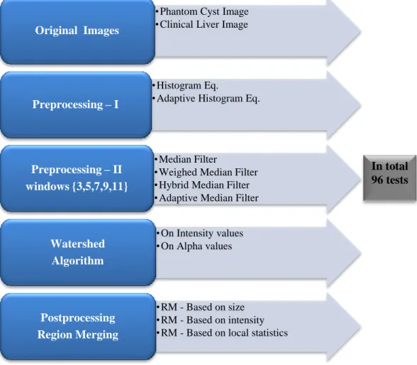
The overall structure of the work done in this thesis can be illustrated as follows. The details of each component is later given in Figure 6.1.
Figure 1.1 :The overall structure of the work done in this thesis.
Based on this schema, each component of our procedure is tested through extensive experiments as summarized in Section 6. Section 7 presents the conclusions and Section 8 lists a number of areas with potential improvement for future work.
1.2Literature Review
There exist a wide range of ultrasound image segmentation methods in the literature [5]. However, the segmentation of brain tissue has different requirements compared to the segmentation of liver. Therefore, the existing methods can be classified
3
according to their clinical application such as cardiology, breast cancer, intravascular diseases etc. A comprehensive overview of segmentation algorithms based on this classification can be found in [4]. Segmentation methods are introduced based on detection of similarity or detection of discontinuity criteria. The detection of similarity is region-based according to a predefined criterion and the detection of the discontinuity is based on sudden changes in the intensity levels. Based on the papers [6,7,8] segmentation methods can be grouped as follows.
Edge based segmentation methods aim to detect edges between different regions by using the information that intensity levels change on the edges. Edge detection based methods (e.g., Sobel operator, Canny operator, Laplace operator [1]) cannot always create closed contours. They also require high image quality, which is not possible for ultrasound images. Therefore, these methods are not sufficient.
Random field based segmentation methods can be Markov Random Field (MRF) and Gibbs Random Field models. In these methods, intensity values of pixels are modelled as a random variable, which have a probability distribution function. MRF algorithm consists of neighborhood definition, energy function, which is minimized by gradient descent, simulated annealing etc., and parameter estimation for maximum a posteriori probability.
Partial differential equation based segmentation (deformable models) uses curves that follow smoothness and object boundary knowledge which are ruled by energy functions. Deformable models are divided into two types as parametric deformable models and geometric deformable models. For instance, active contour model, also known as snake model, is a type of parametric deformable models. Snake model uses both regional and border knowledge. Its energy function includes internal and external energy terms. Internal energy is the sum of elastic and bending energy. Elastic energy makes the snake act like membrane and controls the rigidity of the contour while bending energy makes the snake act like thin plate and responsible for shrinking of the contour. External energy is derived from the image and it gets the smaller value at the region of interest. When the sum of energy functions are minimized, that curve represents boundary of the regions. The drawbacks of this method are that it strongly depends on the initial position of the snake and it has high computational complexity [6].
4
Geometric deformable models are based on level set method and curve evolution theory. Instead of energy function, curves progress according to geometric measures, which do not include parameters. Curves are denoted as a level set of a higher dimensional function.
Machine Learning based algorithms, segmentation problem is treated as classification problem. In this case, clustering algorithms (K-means, fuzzy C means,
Expectation Maximization, Support Vector Machines) are used. Clustering methods are unsupervised methods, which do not require a training phase. As clustering algorithms neglect the spatial information, they are sensitive to noise. Clustering algorithms also require initialization. Spectral clustering algorithms are based on graph theory using different techniques such as Laplace matrix, eigenvalue decomposition and so on.
Support vector machines with a radial basis function kernel are used to classify different patterns, which are generated by sliding window over entire image as in [9].
Artificial neural networks consist of many parallel nodes, which have weights according to their importance. Artifical neural networks require a training phase where learning weights and connection between nodes are learned.
For machine learning algorithms, feature extraction and training phase are important as segmentation heavily depends on the selected features. Feature extraction and training also influence the computation time of the algorithm. In supervised learning methods, another issue can occur in the training phase when the training over fits to the data, and then the algorithm cannot classify unseen samples accurately. On the contrary, if the training under fits the data, then it is also not sufficient to label new samples. In the case of ultrasound images, it is hard to find varied training data.
Region based segmentation treats objects as regions and tries to find regions based on predefined criteria, for instance intensities, texture properties etc. A region growing algorithm [8] starts from a seed point and regions are expanded according to the neighbors with similar characteristic. In this method, the difficulty is in choosing the initial seed point and setting a criteria for growth. In region splitting and merging algorithm [8], the image is first partitioned into areas, and then, merging or splitting is applied according to a defined split/merge rule.
5
Threshold methods are used to separate different gray levels. They can be classified as global threshold, local threshold, and dynamic threshold methods. Threshold methods are susceptible to the noise; hence, they are used together with other methods.
There are several watershed algorithms used for ultrasound image segmentation [10, 11], most of which use the immersion-based watershed algorithm. These watershed algorithms are both edge and region based. The watershed algorithm results in over segmentation and the differences between these approaches are due to the different region merging methods that follow the watershed approach.
In [10], the size of regions, i.e., the number of pixels in the region, is utilized for region merging. The idea is to merge the small regions together based on some threshold values as stopping criteria.
In [11], three different criteria are used for the region merging algorithm. Their criteria are edge information, gray level information and relationship between neighbor regions.
Besides immersion-based watershed algorithm, marker-controlled watershed algorithms are also proposed to deal with the oversegmentation problem on ultrasound images [12,13].
Finally, it is worth mentioning that image segmentation algorithms are hard to evaluate and compare with each other. One possibility is that algorithms can be evaluated on phantom images, for which the features are already known. Another alternative is to use a ground truth image, which can be segmented manually by experts. However, note also that this is human-biased and time-consuming. Finally, unsupervised evaluation methods such as stand-alone evaluation [14], empirical goodness method, intra- and inter-region variance, performance vector, internal and external contrast do not require a reference image. How to compare the different algorithms in the absence of ground truth is studied in detail in [15].
7 WHAT IS ULTRASOUND?
2.
This section covers some background information regarding ultrasound imaging. It starts with a description of some of the properties of ultrasound waves and then presents the principles and modalities of ultrasound imaging systems. More information on ultrasound imaging can be found in [16].
2.1Properties of Ultrasound
Ultrasound (US) is essentially sound with a frequency above 20 kHz, which is not audible for human hearing and needs a medium such as tissue to propagate. US waves are longitudinal waves, which means that their motion is parallel to the direction of the energy transfer.
US waves can be explained in terms of frequency, wavelength, velocity, intensity, and power features [17]. Frequency of the ultrasound waves is proportional to the speed of sound in a tissue while inversely related to wavelength. This relation is shown in the equation (2.1) where is frequency, is velocity and is wavelength.
(2.1)
It should be noted that propagation speed does not depend on frequency and wavelength. It is solely based on medium properties that the wave propagates through medium. Mathematical description of the propagation speed is given as.
√ (2.2)
where is the velocity of sound, is the density in the medium, and is the measure of stiffness, which means resistance for not being deformed when wave is compressed. In summary, propagation speed is related to density and compressibility while speed in the medium is related to the frequency and wavelength.
8
Intensity of the ultrasound waves is related to energy transportation while waves propagate in medium. The average intensity corresponds to the power term. This can be interpreted that intensity of ultrasound waves are proportional to their power. However it is inversely proportional to area of the waves. In acoustics, decibel (dB) scale is used to represent the intensity.
Power in ultrasound denotes the rate of generated and transferred energy by the acoustic wave per time. [18].
2.2Ultrasound Imaging
Conceptually, ultrasound imaging consists of sending acoustic pulse with high frequency through the body, and then transforming the reflected echoes into electric signals, which are converted into ultrasound images.
An ultrasound system consists of the pulse generator, transducer, amplifier, scan convertor, image memory, image display and recording system [19]. Simplified block diagram of ultrasound imaging system is shown in the Figure 2.1.
Figure 2.1 : Block diagram of an ultrasound imaging system.
The first requirement of the system is to generate the ultrasonic waves which are transmitted into the body. A transducer based on piezoelectric principle is used for
9
this purpose. Piezoelectric materials have the property that when mechanical stress is applied, electric field is produced and vice versa. In order to create waves, short duration voltage pulses are applied to the transducer. After the waves are generated, the transducer acts as a receiver. In receiver mode, the transducer collects the waves which are reflected back due to the interaction between waves and tissues. Then a transmitter connects the returning waves (echo) to an electronic signal that is processed and displayed.
Transducers used for medical imaging are arrays. Their commonly used types are linear transducers, curved linear transducers and phased array transducers.
The linear transducers consist of a large number of piezoelectric elements arranged in parallel lines. The parallel positoning of scan lines produces a rectangular image with the same width as the transducers. This kind of transducer is preferred for vascular and some abdominal imaging. The disadvantage of linear transducer is that it only focuses on the image plane which causes image thickness. This has negative impact on spatial resolution.
In the curved linear transducer, piezoelectric elements are located on curve instead of straight lines as in the linear transducer. Image shape of the curved linear transducers is trapezoidal. When the search depth increases namely large tissue structures are examined, for instance in abdominal applications, the curved linear transducers are employed.
The phased array transducer has an array of piezoelectric elements similar to the linear array. Ultrasound pulses are transmitted in straight line which are perpendicular to the transducer unlike linear array transducer. This assembly generates triangular-shaped image. These kind of transducers are designed for cardiac applications. Its disadvantage is that, its procedure is more time-consuming compared to 2-D alternatives because of 3-D properties. These transducer types are shown as example based on [20] in the Figure 2.2.
10
Figure 2.2 :Transducer types based on [20].
The quality of the ultrasound image is related to resolution. Resolution term in ultrasound images can be defined as ability to distinguish different point and has types such as spatial, lateral and temporal resolution. Spatial resolution describes this ability in space and is subcategorized as axial and lateral resolution. Axial resolution represents the resolution property along the ultrasound propagation direction. It is determined by the length of the ultrasound pulse. Lateral resolution denotes the ability of the system to discriminate two points in the direction perpendicular to the direction of propagation. In ultrasound imaging, axial resolution is better than lateral resolution [21]. Temporal resolution is the ability to detect moving objects over time and this can be interpreted as frame rate for medical ultrasound applications. Linear Transducer Phased Transducer Curved Linear Transducer
11 2.2.1 Ultrasound – tissue interaction
As ultrasound waves are directed into body, it causes different interactions due to the characteristic difference of tissues. These observed interactions are reflection,
refraction, scattering, diffraction and interference [19,21]. Briefly, they can be explained as follows:
Reflection occurs at the boundaries between different tissue types because of acoustic impedance property. Acoustic impedance is based on medium density and propagation speed, and calculated as a product of these terms. Once meeting with a tissue, some waves can be transmitted into other tissue while some are reflected back. The amplitude of the waves is related to acoustic impedance change. Specifically, small acoustic impedance differences produce weak echoes and vice-versa. Another cause of reflection is due to the fact that interfaces are larger compared to the wavelength of ultrasound.
Refraction is defined as direction changes of waves when they hit the boundary of organs. Direction does not change under the condition that speed of sound remains same for both media. Its adverse effect is misleading localization of a structure on an US image. The speed of sound is low in fat and high in soft tissues.
Scattering takes place when US waves interact with tissues that are smaller than ultrasound’s wavelength. It is directly proportional to frequency, which means it rapidly increases when frequency of ultrasound increases. Because of the spatial arrangement of the scatterers, there are two types of scattering. If the scatterers produce periodicity in the echo waves, it is called coherent scattering. If the scatterers are spatially random distributed, it leads to the diffuse scattering. Scattered power is proportional to a tissue size, which is smaller than wavelength, and inversely proportional to the wavelength.
Diffraction occurs in the case of wave spreading through small holes. The amount of diffraction depends on size of this hole and wavelength of waves.
Interference yields phase information when waves align with each other. Main cause for interference is scattering. Interference varies as constructive and
destructive. If waves are in the same phase, it causes constructive interference, which arises from increased amplitude. If waves are out of phase, they are subject to
12
destructive interference, which leads to a complex wave summation. Focusing of the US beam in real time imaging is based on the principle of wave interference.
Attenuation results in absorption, reflections and destructive interference. Absorption of ultrasound beam is defined as energy conversion process, primarily heat. Attenuation increases proportionally with frequency.
2.2.2 Ultrasound modes
Ultrasound scanning modes mainly varies as A- mode and B- mode [22]. Other modes such as M-, T-, color coded, and Doppler mode are derived from these main modalities. Commonly used modes are outlined below based on [21,22].
A-mode scanning is named based on amplitude, and it is the earliest mode of ultrasound which is no longer used. In this mode, reflected signal is measured and displayed as a continuous signal. The display of the tissue is obtained in one dimension.
B-mode scanning refers to brightness mode. In this mode, reflected waves are demonstrated as a 2D gray level image, which is obtained in many different directions. Amplitude of reflected waves are denoted by gray levels that varies from black to white.
Motion mode, M–mode, is similar to A–mode scanning. Results are displayed according to the lines, which are obtained consecutively across time. The vertical axis is the depth of the tissue in meters, while horizontal axis is time in seconds. Unlike B-mode, in M-mode display acoustic axis is fixed.
T-mode display denotes transmission mode scanning. In this mode, there is difference between receiver and transmitter of the ultrasonic wave unlike B-mode.
Information about the tissues are obtained by transmission instead of reflection. This mode is used for breast scanning.
Doppler mode provides velocity sampling at different depths and positions. Several types of doppler systems are used in medical diagnosis such as continuous wave Doppler, pulsed wave Doppler, duplex ultrasound and color flow duplex doppler.
13
PREPROCESSING OF ULTRASOUND IMAGES 3.
Preprocessing is an important step of digital image processing. It reduces the artifacts and provides an initial enhancement in the quality of the image. For ultrasound images, the preprocessing method is aimed at speckle noise reduction, also known as
despeckling [22].
Due to coherent energy, speckle noise inherently occurs in ultrasound images. Speckle degrades the image quality in terms of resolution and contrast. This has a negative impact on both diagnostic examination and image processing methods, and hence, needs to be eliminated.
It should be noted that speckle pattern is mostly asserted as noise, which needs to be eliminated, but on the other hand, it also includes important information about tissues [23]. That is, there exists a trade-off between reducing noise and losing information about the image.
Our preprocessing procedure has two components: (i) histogram equalization methods, and (ii) filtering methods. This section first presents speckle noise, its physical properties, and reviews the methods used to reduce it. Then, the details of our preprocessing methods are described.
3.1Speckle Noise
As previously mentioned, when the beam strikes a tissue, whose size is bigger compared to the wavelength of the beam, it results in scattering. When scatterers are in random phase, coherent summation of backscatterers generate light and dark spots, which is called as speckle. Scatterer numbers per region of the object, known as the
scatter number density (SND), determines the pattern of speckle. This pattern is repeatable, which means that under the same conditions, it is obtained identically in the same way [24].
Speckle noise occurs in many procedures including; coherent radiation, synthetic aperture radar (SAR), laser and medical ultrasound imaging, which is the focus of
14
this thesis. In ultrasound imaging, speckle noise types are divided into four types based on SND and deterministic components:
Fully developed form, has large number of scatterers without deterministic component. Amplitude of backscatters is modeled as Rayleigh distribution [24,25] and their phases are distributed uniformly between - and + .
Fully resolved form, which has deterministic component in addition to large number of scatterers and modeled as Rice distribution, where echo signal’s mean is shifted away from the origin [26].
Partially developed form, which has small number of scatterers unlike fully types with non-existence of deterministic component and it has K-distribution model [27,28].
Partially resolved form has features of both small number of scatters and deterministic component. It is represented as K-Homodyne distribution [28]. There are many proposed methods for modeling the speckle noise [22]. Fully speckle condition is the most popular in ultrasound images [30], as such; the speckle noise model is defined according to it. The study presented in [30] suggests that the assumptions behind the Rayleigh distribution are better suited to model pixel intensities in homogenous areas compared to other distributions such as K-, Nakagami-, and Rician Inverse Gaussian distribution. Rayleigh distribution assumes that the mean value is proportional to the standard deviation with . This implies that speckle noise can be modeled as multiplicative with original image. The variance is related to image intensity in such way that brighter areas include more noise power compared to dark areas. Ultrasound images are displayed on logarithmic scale, and hence the speckle mean becomes proportional to variance [31-33].
( ) ( ) √ ( ) ( ) (3.1)
Where (), () and () represent the observed signal, noise-free signal, and noise respectively. This model implies that, the image variance is proportional to mean on homogeneous regions where () can be assumed as constant.
15 3.2Speckle Reduction Methods
In the literature, various methods are proposed to reduce speckle noise. Mainly, these methods can be grouped as linear filtering, non-linear filtering, diffusion based filtering, and wavelet filtering [21].
Some of the linear filters are used for speckle reduction are Lee [34], Kuan [35] and Frost [36]. The principles behind these filters are based on a sliding window (kernel) over the image. Lee filter is based on minimum mean square error. In this filter, if the variance in window is low, the central pixel of the window is replaced with the local mean of pixels inside the window. Contrarily, if the variance is high, Kuan filter is used which is a generalized form of Lee filter under non-stationary mean and variance assumption. In Frost filter, the image is convolved with exponential impulse response. This filter performs similar to averaging in low variance areas, and in high variance areas, it instead preserves sharp features.
Regarding nonlinear filters, homomorphic filters, maximum homogeneity over pixel neighborhood filtering (MHOPNF) can be given as an example.
Homomorphic filters [37] are based on Fourier transform including a logarithmic mapping that converts multiplicative speckle noise form to additive noise. After obtaining image with additive noise, high pass filters in logarithmic domain are applied in order to remove the noise.
In MHOPNF [38], by sliding the window, the center pixel is updated based on the most homogenous neighborhood around which is calculated for every pixel in the image. This filter does not require any parameters or threshold to be tuned. Diffusion filtering varies as anisotropic diffusion filtering, speckle-reducing anisotropic diffusion (SRAD) and coherent diffusion.
Anisotropic diffusion filter [39] uses nonlinear partial differential equation (PDE) to remove speckle. This method is capable of reducing speckle and at the same time strengthening the edge information with edge detection function.
SRAD [40] utilizes instantaneous coefficient of variation instead of gradient-based edge detector in PDE of the anisotropic diffusion filter. This method is applied on image, which does not have logarithmic compression.
16
Coherent diffusion [41] is proposed for coherent enhancement. It can be treated as a hybrid method that combines isotropic diffusion, anisotropic diffusion and mean curvature motion.
In wavelet filtering [42], the image is transformed into wavelet domain and noise is removed based on wavelet coefficients.
As noted in [22], most of the proposed speckle reduction methods have their limitations. First of all, they are sensitively dependent on the window size and the shape. That means, the choice of window size is critical. In case, the window is too large, it smooths overly, as a result edge information is lost due to blurring. On the other hand, if the window is too small, then it does not sufficiently smooth the image so as to reduce speckle noise. Secondly, some methods are based on a threshold value which should be set properly according to the image at hand. When it is not chosen correctly, it leads to noisy boundaries. Both quantitative metrics (SNR, PSNR etc.) and visual assessments by experts are used for evaluation but differences between such measurements prevent objective comparison about speckle filtering methods.
In this thesis, speckle reduction methods are used as preprocessing which consist of two parts. First, in order to increase dynamic range of pixel values, histogram equalization and its adaptive version are used. Then, since speckle noise can be considered as a salt and pepper noise, the median filters are applied as a second step. In particular, median filter and its variants such as hybrid median filter, weighted median filter and adaptive median filter are used. The next section describes these methods.
3.3Preprocessing – I: Histogram Equalization
Firstly, histogram of an image denotes the frequency of occurrence of the pixel values. Mathematically, it represents probability distribution of the pixel based on divided value of number of specific k th pixels to total number of pixels.
Histogram of the image is interpreted in a way that if image has a narrow histogram, its contrast is low, namely the differences between maximum and minimum intensities is small. For visibility and quality of the image, a large histogram is
17
demanded [43]. Another knowledge is obtained form histogram is number of peaks denotes the number of regions which can be used to analyze the image.
Histogram equalization represents the histogram as a cumulative distribution which is summation of the pixel distributions. This accomplishes to make pixels uniformly distributed. In the equations below, former one denotes the calculation of the histogram and latter one represents the transformation of the pixels distribution namely histogram equalization is shown.
( ) (3.2) ∑ ( ) ∑ (3.3)
Where is kth gray level, ( ) is its probability density function. In next equation, is the output image when each pixel with level is mapped. For both equation is number of kth pixels, is total number of pixels.
Histogram equalization enhances the image globally but if local enhancement is required then its extension, namely adaptive histogram equalization, is used. In adaptive histogram equalization, histogram equalization is calculated on small regions (tiles) rather than entire image. To avoid noise amplification, contrast expansion is limited. In the end, histogram equalized tiles are combined by using bilinear interpolation.
3.4Preprocessing – II: Filtering Methods 3.4.1 Median filter
Median filter [40] is linear and categorized as order statistic filter. It is non-linear because it does not satisfy the following superposition property:
[ ( ) ( )] ( ) ( ) (3.4)
where ( ) and ( ) represent the images. This fact should be taken into account if summing of filtered images is considered.
18
Median filter is applied in the spatial domain by shifting a window through the image, where the center pixel of input image is replaced with the median value of ascendingly sorted pixel values inside the window. This step is repeated for all pixels, yielding the filtered image. For pixels at the edge, the window size exceeds image, therefore zero padding or symmetrical padding is used. Since the median value is used, the window size is mostly chosen as an odd number. Otherwise, after sorting the pixels, the average of two middle values has to be calculated.
With this method, outliers, which have high intensities in the image, are suppressed, and variances of intensities are reduced. Therefore, its effect on image can be interpreted as smoothing. However, it should be noted that smoothing causes blurring which is an undesired effect.
The performance of the median filter depends on the window size and the type of noise. In terms of window size, the median filter can remove noise correctly if the number of noisy pixels in the window is less than (n2+1)/2 where the window size is
n x n [45]. In terms of the noise type, in [44] it is shown that median filters are capable of dealing with multiplicative and impulsive noise.
There are various variants of median filtering techniques including directional median, iterative median, recursive median, switching median, sequential median filters so on. Apart from the median filter, in this study, hybrid, weighted and adaptive versions are used for preprocessing, as outlined next.
3.4.2 Weighted median filter
While in median filter, all pixels have equal weights, in weighted median (WM) filter [46], the window is weighted using integer/non-integer coefficients for specific filter positions. WM filter can be defined in two different, but equivalent ways, based on the choice for selecting the weights, as shown in [46]:
Definition I: weights are assumed as non-negative integer values. The first pixel inside the filter window is replicated n times where n corresponds to weights in filter window. Then, the replicated array is sorted in ascending order, and lastly, the median value of array is chosen. This process can be described as:
19
Where ( ) corresponds to weights in the filter window, ( ) is pixel values and symbolizes duplication operation. The result of this equation is new pixel value in the filtered image.
Definition II: weights are assumed to be positive non-integer. Let the weighted median value of X set of pixels in window be , which minimizes the following equation.
( ) ∑
(3.6)
Piecewise linear and convex properties of ( )provides that is certainly one of the samples of .
Calculation WM of pixels is carried out as follows: sort the pixel values in the window in ascending order, which also changes the order of weights. After sorting pixels and reordering, weights are summed up starting from first element. This iterative summation stops when the sum of the weights considered so far, exceeds half of the total sum of weights. The output value for WM is the pixel corresponding to the last weight added.
In this study, Definition – I, is used for the WM filtering. The weights of the filter are chosen in such way that pixels further from center contribute less.
3.4.3 Hybrid median filter
Hybrid median filter [43] is a multiple ranking filter, specially based on applying median filter several times with different positioning of the filter.
In this method, center pixel value within window of filtered image is assigned as follows: First, median value is chosen among the horizontal and the vertical neighbors of the center pixel. Second, the diagonal neighbors’ median value is found. Median values, obtained in first and second step, are ranked with the central pixel and final median value is determined from these three median values.
For example, given a window of size 3x3 where C is the center pixel and its diagonal neighbors are denoted by D, its horizontal neigbors are denoted by H and its vertical neighbors are denoted by V.
20
Figure 3.1 : Illustration for computation of hybrid median filter, adapted from [43]. Based on the figure above, the hybrid median filter is calculated as follows.
Step 1: medianN= findMedian (V1 V2 C H1 H2 ) Step 2: medianD = findMedian (D1 D2 C D3 D4 )
Step 3: hybrid median = findMedian( medianN, medianD, C)
Compare to conventional median filter, advantages of hybrid median filter can be considered as less smoothing, better preservation for lines and edges, and faster due to the less computation [1].
3.4.4 Adaptive median filter
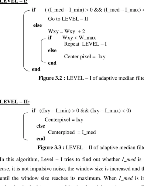
In adaptive median filter [1], the window size changes during the filtering process based on the local features within window. The goal of this filter is to remove impulsive noise while other noise types are suppressed. Based on the description given in [1], the following notation and algorithm is used to describe the steps of this filtering.
Notation:
Wxy = Window at (x,y) where (x,y) is window center W_max = Maximum window size
I_min = Minimum gray level value in Wxy I_max = Maximum gray level value in Wxy I_med = Median gray level value in Wxy Ixy = Gray level value at (x,y) coordinate
Step 1
Step 2
21 LEVEL – I:
if ( (I_med – I_min) > 0 && (I_med – I_max) < 0) ) Go to LEVEL – II else Wxy = Wxy + 2 if Wxy < W_max Repeat LEVEL – I else
Center pixel = Ixy end
end
Figure 3.2 :LEVEL – I of adaptive median filter.
LEVEL – II:
if ((Ixy – I_min) > 0 && (Ixy – I_max) < 0) Centerpixel = Ixy
else
Centerpixed = I_med end
Figure 3.3 : LEVEL – II of adaptive median filter.
In this algorithm, Level – I tries to find out whether I_med is impulsive noise. In case, it is not impulsive noise, the window size is increased and this level is repeated until the window size reaches its maximum. When I_med is impulsive noise, Ixy
value is checked in terms of having impulsive noise or not. When Ixy is not an impulsive, then Ixy is returned as output, and otherwise, I_med is returned as output.
23 THE WATERSHED ALGORITHM 4.
The watershed concept for image processing is used as segmentation method which is region based. The algorithm is based on an analogy from geography where the watersheds form the lines that separate drainage areas, which are called catchment basin, of different rivers [47].
The input image is treated as a topographical surface where its gray level values considered as altitude because of the intensity differences. The catchment basins represent regions of segmented objects, while watershed lines are boundaries between different catchment basins.
There exists a number of different watershed algorithms. This thesis employs the immersion-based algorithm. An overview of existing watershed algorithms is provided in the next section. A more detailed survey on watershed algorithm can be found in [47].
4.1An Overview of Watershed Algorithms
The idea of using the watershed method is first proposed by Digabel and Lantuéjou [48] by using binary image for contour detection. Later, Beucher and Lantuéjou [49] proposed extended watershed method to be used in gray scale images. There are many definitions for the watershed algorithms in literature. The watershed algorithms for the discrete case can be classified mainly in five groups based on [50].
The first definition is based on flooding, which simulates the immersion of the topographical surfaces with water. It is a recursive process where regions expand based on skeleton by influence zone. The algorithm used in this thesis follows the flooding definition, hence, this is explained in more detail in the next section.
The second definition is based on topological distance watershed where topographical distance between any two pixel is the minimum path among all topographical distances. The important point here is that the paths between pixels should be the steepest descent. The watershed based on topographical distance is
24
described over a cost function. The cost function between any two pixel is computed as summation of geodesic distances between middle pixels. This function determines that pixels belong to unique minimum, hence, catchment basins. If pixels belong to more than one basin, it is labeled as watershed.
The third definition is based on path-cost minimization algorithms. In this case, pixels are grouped as catchment basin when topographical distance is precisely small to the regional minimum. In image foresting transform, the image is described as a weighted graph. Then, a forest of minimum path-trees is created by path-cost minimization. Trees in this forest correspond to basins.
The fourth definition is based on local condition watershed algorithms that assign the label of minimum points to each pixel instead of building watershed lines. It is derived from topographical distance which does not have unique label restriction anymore. Locality means that image are subdivided into blocks and labelling is performed over evey block separately in order to get globally good results.
The fifth one is based on minimum spanning forest, the watershed is constructed as a weighted graph where its nodes are catchment basins corresponding to regional minima.
Besides these definitions, another source of difference is due to the strategies used to scan the pixels. These strategies are immersion, hierarchical queue, shortest path,
hill climbing, sequential scanning, connected components, union-find, chain code,
tie-zone, order invariant toboggan and immersion and watershed cut [51].
Noise and local inhomogenity have negative impact over the watershed algorithms resulting in oversegmentation. Additional knowledge such as gradient and color might be used to overcome this issue, which can be embedded in marker-controlled
watershed algorithm [1]. These markers are connected components that contain a priori knowledge for segmentation. They can be classified as internal and external
markers. Internal markers are applied to get information about region of interest, which includes the objects, that is, the foreground. External markers are used to gain an understanding of the outside of the object, that is, the background. In addition, markers can be assigned manually or automatically.
Before describing the technical details of the immersion-based flooding algorithm, namely; the Vincent-Soille algorithm, some definitions are given in the next section.
25 4.2Definitions
First of all, description of a gray scale image is a triple ( ) where ( ) is a graph is a function which assigns an integer to each pixel , . In view of this definition, ( ) represents the gray level value or altitude in watershed algorithms.
Neighborhood: The neighborhood can be defined in three ways, 4-, diagonal and 8-neighborhood. For a given pixel p(x, y);
The 4-neighbors are:
( ) ( ) ( ) ( ) (4.1)
The 4-diagonal neighbors are:
( ) ( ) ( ) ( ) (4.2)
The 8-neighborhood consists of both 4- and 4-diagonal neighbours.
Adjaceny: If two pixels are neigbors and their gray level values satify same similarity criterion, then these pixels are assumed to be adjacent.
Path: A path is a sequence of pixels. For example, the path from pixel p to pixel q
with length Ɩ is such that; (p0, p1, …. ,pƖ-1, pƖ) where p0 = p, pƖ = q, and pixels pi and pi-1 are adjacent for 1 ≤ i ≤ Ɩ. If pixel values do not increase in the path, the path is called a descending path. The opposite condition is ascending path where pixels values do not decrease.
Connected Component: A connected component is a subset of pixels in an image where there is a path between any two pixel.
Level Component: A connected component in which the pixels have same value at specific level h is known as a level component. The level h is known as altitude.
Regional Minimum: A connected component of pixels under the condition that there is no pixel with a lower value than h.
Plateau: A plateau is a connected component in which pixels have constant gray value.
26
Threshold: Threshold is set of values which are lower than h. Formally;
( ) (4.3)
in which symbolizes gray level values in pixels .
Geodesic Distance: The geodesic distance dA(x,y) is defined for two points x and y in A where A d, and it represents the length of the shortest path among all paths from x and y within A.
Geodesic Influence Zone: Let B be a subset of A where B is composed of n connected components Bi, i = 1,...,n . Then the geodesic influence zone of Bi in A is defined as;
( ) [ ] ( ) ( ) (4.4)
This equation can be interpreted as the geodesic influence zone of Bi is the set of points in A that their distance is the closest to A among all Bi. The union of the geodesic influence zone of the all connected component is;
( ) ⋃ ( )
(4.5)
Skeleton by Influence Zones (SKIZ): The skeleton influence zone is defined as the complement set of the geodesic influence zone of all components. Based on the equation (4.5);
( ) ( ) (4.6)
That means geodesic SKIZ is the boundaries of all geodesic influence zones.
Catchment Basins: The catchment basins are regions in S surface, whichcontain only one regional minimum. ( ) of minimum among minimum set of where . This means points in ( ) is closer to than any other regional minimum .
27
( ) ( ) ( ) ( ) ( ) (4.7)
In the equation above, denotes gray level values in , represents distance between minima.
Watershed: A watershed is the set of points which do not belong to any catchment basin.
( ) ⋃ ( ) (4.8)
4.3The Vincent – Soille Algorithm
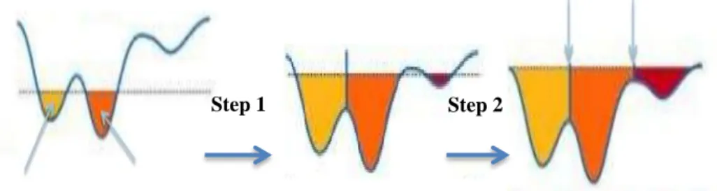
The Vincent – Soille algorithm [52] is an immersion-based watershed algorithm. The analogy behind this algorithm is shown in Figure 4.1 which is adapted from [53].
Figure 4.1 : Illustration for the immersion-based watershed algorithm.
The basins are filled with water starting from the local minimum in every basin. When the water sources different basins meet, dams are built so as to prevent merging. Flooding is stopped when the water level reaches the highest peak. In this analogy, catchment basins symbolize different objects and dams correspond to watershed lines which separates the catchment basins.
Catchment Basins
Watershed Lines
Step 2 Step 1
28
Algorithmic definition of immersion can be shown with the following recursion [47]; ( )
(4.9a)
[ ( )\ ] [ ) (4.9b)
The definitions of the terms used in equation (4.9a) and (4.9b) are:
where f is digital gray level image whose minimum and maximum intensity values are shown by hmin, hmax.
represents computed combination of basins at level h
is threshold set for level h+1. This threshold can be interpreted as a new minimum or expansion of a basin in .
denotes the combination all all regional minima at level h
( ) is computation of the geodesic influence zone of within and it is a updating criteria for .
( ) D \ (4.10)
4.4The Implementation of the Vincent – Soille Algorithm
The actual implementation of the recursive algorithm in practice can be summarized in two steps, the sorting step and the flooding step.
In the first step, pixel values are sorted in an ascending order which is later used to access pixels directly for specific level h. The flooding step consists of fast breadth- first scanning of all pixels from hmin to hmax and progress for every gray level by using a First-In-First-Out (FIFO) data structure called queue. All pixels which have neighbours with lower than current level h are added in the queue. These pixels are labelled with the minimum label of their neighbor. When the flooding is completed until level h, this implies that pixels which have equal or less gray level to h are assigned to a unique label.
29
In the next step, pixels in h+1 have two possibilities either being the catchment basin of h or a new local minimum at level h+1. Some of the pixels in h+1 level that are neighbours of h level are added into queue. The pixels from the queue are processed sequentially. Pixels in the queue that are not assigned to any existing label, generate new catchment basins. All catchment basins have unique label representing different regions in the image. When two catchment basins come to the point where they can join, a watershed line is generated which a special value. If the point labelled as watershed, then it is not considered again in the next iteration.
The watershed algorithm works well if the objects are in local minima. However, if there are many minima in the image unrelated to regions of the object, then oversegmentation, which is the main issue of watershed algorithms in general, occurs. Besides that, noise in the image might also cause oversegmentation [54]. In this thesis, to address the oversegmentation problem, region merging algorithms based on various criteria, which are described in the next section, are proposed as a postprocessing step.
31
POSTPROCESSING OF ULTRASOUND IMAGES 5.
The watershed algorithms suffer from oversegmentation leading to insufficient segmentation results. To deal with oversegmentation problem, a region merging algorithm is based on the following criteria is introduced.
1. The size of the regions
2. The difference in intensity of regions 3. Statistical information about the regions
Before explaining the details of the region merging algorithm, let us first review how the regions are obtained.
5.1Extracting the Regions
Once the watershed algorithm is executed on a given ultrasound image, a matrix, which is of the same size as the input image is produced it also includes labels. This matrix is called the label matrix. Labels are integer values from 1 to n, where n
denotes the maximum value of labels. A group of pixels that have the same label defines a region. That is, the number of labels also represents the number of regions. Besides the labels, the matrix also includes zero entries which are interpreted as the watershed lines that separate different regions from each other.
In order to define the association of the regions precisely, a graph theoretic data structure called region adjaceny graph (RAG) [55] is employed. RAG creates a graph with nodes N = { N1,N2, ..., Nk } where Ni corresponds to region Ri. If there exists a watershed line between regions Ri and Rj, then they are adjacent to each other, which is represented by creating an edge between the corresponding Ni and Nj nodes. Adjacency between nodes can be described in different ways such as 4-neighborhood, 8-neighborhood and etc.
![Figure 2.2 : Transducer types based on [20].](https://thumb-us.123doks.com/thumbv2/123dok_us/9069956.2805212/36.892.168.652.93.702/figure-transducer-types-based.webp)
![Figure 3.1 : Illustration for computation of hybrid median filter, adapted from [43].](https://thumb-us.123doks.com/thumbv2/123dok_us/9069956.2805212/46.892.176.649.106.409/figure-illustration-computation-hybrid-median-filter-adapted.webp)