A Survey of Visualization Pipelines
Kenneth Moreland,
Member, IEEE
Abstract—The most common abstraction used by visualization libraries and applications today is what is known as the visualization pipeline. The visualization pipeline provides a mechanism to encapsulate algorithms and then couple them together in a variety of ways. The visualization pipeline has been in existence for over twenty years, and over this time many variations and improvements have been proposed. This paper provides a literature review of the most prevalent features of visualization pipelines and some of the most recent research directions.
Index Terms—visualization pipelines, dataflow networks, event driven, push model, demand driven, pull model, central control, distributed control, pipeline executive, out-of-core streaming, temporal visualization, pipeline contracts, prioritized streaming, query-driven visualization, parallel visualization, task parallelism, pipeline parallelism, data parallelism, rendering, hybrid parallel, provenance, scheduling, in situ visualization, functional field model, MapReduce, domain specific languages
F
1
I
NTRODUCTIONT
HE field of scientific visualization was launched with the 1987 National Science Foundation Visualization in Scientific Computing workshop report [1], and some of the first proposed frameworks used a visualization pipeline for managing the ingestion, transformation, display, and recording of data [2], [3]. The combination of simplicity and power makes the visualization pipeline still the most prevalent metaphor encountered today.The visualization pipeline provides the key structure in many visualization development systems built over the years such as the Application Visualization System (AVS) [4], DataVis [5], apE [6], Iris Explorer [7], VIS-AGE [8], OpenDX [9], SCIRun [10], and the Visualization Toolkit (VTK) [11]. Similar pipeline structures are also ex-tensively used in the related fields of computer graph-ics [2], [12], rendering shaders [13], [14], [15], and image processing [16], [17], [18], [19]. Visualization applications like ParaView [20], VisTrails [21], and Mayavi [22] allow end users to build visualization pipelines with graphical user interface representations. The visualization pipeline is also used internally in a number of other applications including VisIt [23], VolView [24], OsiriX [25], 3D Slicer [26], and BioImageXD [27].
In this paper we review the visualization pipeline. We begin with a basic description of what the visualization pipeline is and then move to advancements introduced over the years and current research.
2
B
ASICV
ISUALIZATIONP
IPELINESA visualization pipeline embodies a dataflow network in which computation is described as a collection of executable modulesthat are connected in a directed graph representing how data moves between modules. There are three types of modules: sources, filters, and sinks. A source module produces data that it makes available through an output. File readers and synthetic data generators are typical source K. Moreland is with Sandia National Laboratories, PO Box 5800, MS 1326, Albuquerque, NM 87185-1326. E-mail: kmorel@sandia.gov
Digital Object Identifier no. 10.1109/TVCG.2012.133. c
2013 IEEE
modules. A sink module accepts data through aninputand performs an operation with no further result (as far as the pipeline is concerned). Typical sinks are file writers and rendering modules that provide images to a user interface. A filter module has at least one input from which it transforms data and provides results through at least one output.
The intention is to encapsulate algorithms in interchange-able source, filter, and sink modules with generic connection ports (inputs and outputs). An output from one module can be connected to the input from another module such that the results of one algorithm become the inputs to another algorithm. These connected modules form a pipeline. Fig. 1 demonstrates a simple but common pipeline featuring a file reader (source), an isosurface generator [28] (filter), and an image renderer (sink).
Isosurface
Render
Read
Fig. 1: A simple visualization pipeline.
Pipeline modules are highly interchangeable. Any two modules can be connected so long as the data in the output is compatible with the expected data of the downstream input. Pipelines can be arbitrarily deep. Pipelines can also branch. A fan out occurs when the output of one module is connected to the inputs of multiple other modules. A fan in occurs when a module accepts multiple inputs that can come from separate module outputs. Fig. 2 demonstrates a pipeline with branching.
These diagrams are typical representations of pipeline structure: blocks representing modules connected by arrows representing the direction in which data flows. In Fig. 1 and Fig. 2, data clearly originates in the read module and ter-minates in the render module. However, keep in mind that this is a logical flow of data. As documented later, data and control can flow in a variety of ways through the network.
Isosurface
Reflect
Read
Render
Streamlines
Glyphs
Tubes
Fig. 2: A visualization pipeline with branching. Intermediate results are shown next to each filter and the final visualization is shown at the bottom. Shuttle data courtesy of the NASA Advanced Supercomputing Division.
However, such deviation can be considered implementation details. From a user’s standpoint, this conceptual flow of data from sources to sinks is sufficient. This paper will always display this same conceptual model of the dataflow network. Where appropriate, new elements will be attached to describe further pipeline features and implementations.
To better scope the contents of this survey, we consider the following formal definition. A visualization pipeline is a dataflow network comprising the following three primary components.
• Modules are functional units. Each module has zero or more input ports that ingest data and an independent number of zero or more output ports that produce data. The function of the module is fixed whereas data entering an input port typically change. Data emitted from the output ports are the result of the module’s function operating on the input data.
• Connections are directional attachments from the out-put port of one module to the inout-put port of another module. Any data emitted from the output port of the connection enter the input port of the connection. Together modules and connections form the nodes and arcs, respectively, of a directional graph. The dataflow network can be configured by defining connections and connections are arbitrary subject to constraints.
• Executionmanagement is inherent in the pipeline. Typi-cally there is a mechanism to invoke execution, but once invoked data automatically flows through the network. For a system or body of research to be considered in
this survey, it must be the embodiment of a visualization pipeline. It must allow the construction of objects that represent modules, and it must provide a means to connect these modules. This definition excludes interfaces that are imperative or functional as well as interfaces based on data structures defining graphical representation such as scene graphs or marks on hierarchies.
This paper is less formal about what it means to be a visualizationpipeline (as opposed to, say, an image pipeline). Suffice it to say that the surveyed literature here are self-declared to have a major component for scientific visualiza-tion.
For more information on using visualization pipelines and the modules they typically contain, consult the documenta-tion for one of the numerous libraries or applicadocumenta-tions using a visualization pipeline [11], [20], [29], [30], [31], [32], [33].
3
E
XECUTIONM
ANAGEMENTThe topology of a pipeline dictates the flow of data and places constraints on the order in which modules can be executed, but it does not determine how or when modules get executed. Visualization pipeline systems can vary signif-icantly in how they manage execution.
3.1 Execution Drivers
The visualization pipeline represents a static network of operations through which data flows. Typical usage en-tails first establishing the visualization pipeline and then
executing the pipeline on one or more data collections. Consequently, the behavior of when modules get executed is a primary feature of visualization pipeline systems. Visual-ization pipelines generally fall under two execution systems: event driven and demand driven.
An event-driven pipeline launches execution as data be-comes available in sources. When new data bebe-comes avail-able in a source, that source module must be alerted. When sources produce data, they push it to the downstream modules and trigger an event to execute them. Those down-stream modules in turn may produce their own data to push to the next module. Because the method of the event-driven pipeline is to push data to the downstream modules, this method is also known as the push model. The event-driven method of execution is useful when applying a visualization pipeline to data that is expected to change over time.
Ademand-driven pipeline launches execution in response to requests for data. Execution is initiated at the bottom of the pipeline in a sink. The sink’s upstream modules satisfy this request by first requesting data from their upstream modules, and so on up to the sources. Once execution reaches a source, it produces data and returns execution back to its downstream modules. The execution eventually unrolls back to the originating sink. Because the method of the demand-driven pipeline is to pull data from the upstream modules, this method is also known as the pull model. The demand-driven method of execution is useful when using a visualization pipeline to provide data to an end user system. For example, the visualization could respond to render requests to update a GUI.
3.2 Caching Intermediate Values
Caching, which saves module execution outputs, is an im-portant feature for both execution methods. In the case of the event-driven pipeline, a module may execute only when data from all inputs is pushed to it. Thus, the execution must know when to cache the data and where to retrieve it when the rest of the data is later pushed.
In the case of the demand-driven pipeline, a module with fan out could receive pull requests from multiple downstream modules during the same original sink request. Rather than execute multiple times, the module can first check to see if the previously computed result is still valid and return that if possible.
Although caching all the intermediate values in a pipeline can remove redundant computation, it also clearly requires more storage. Thus, managing the caching often involves a trade-off between speed and memory. The cost of caching can be mitigated by favoring shallow copies of data from a module’s inputs to its outputs.
3.3 Centralized vs. Distributed Control
The control mechanism for a visualization pipeline can be either centralized or distributed. A centralized control has a single unit managing the execution of all modules in the pipeline. The centralized control has links to all modules, understands their connections, and initiates all execution in the pipeline.
Adistributed controlhas a separate unit for each module in the pipeline. The distributed control unit nominally knows only about a single module and its inputs and outputs. The distributed control unit can initiate execution on only its own module and must send messages to propagate execution elsewhere.
Centralized control is advantageous in that it can per-form a more thorough analysis of the pipeline’s network to more finely control the execution. Such knowledge can be useful in making decisions about caching (described in Section 3.2) and load balancing for parallel execution (described in Section 5). However, the implementation of a centralized control is more complex because of the larger management task. Centralized control can also suffer from scalability problems when applied to large pipelines or across parallel computers. Distributed control, in contrast, has more limited knowledge of the pipeline, but tends to be simpler to implement and manage.
3.4 Interchangeable Executive
Many visualization pipeline implementations have a fixed execution management system. However, such a system can provide more flexibility by separating its execution management into an executive object. The executive object is an independent object that manages pipeline execution. Through polymorphism, different types of execution models can be supported. For example, VTK is designed as a demand-driven pipeline, but with its interchangeable exec-utives it can be converted to an event-driven pipeline, as demonstrated by Vo et al. [34].
Replacing the executive in a pipeline with centralized control is straightforward. The control is, by definition, its own separate unit. In contrast, a distributed control system must have an independent executive object attached to each module in the pipeline. The module objects get relegated to only a function to execute whereas the executive manages pipeline connections, data movement, and execution [35]. 3.5 Out-of-Core Streaming
An out-of-core algorithm (or more formally an external-memory algorithm) is a general algorithmic technique that can be applied when a data set is too large to fit within a computer’s internal memory. When processing data out of core, only a fraction of the data is read from storage at any one time [36]. The results for that region of data are generated and stored, then the next segment of data is read. A rudimentary but effective way of performing out-of-core processing in a visualization pipeline is to read data in pieces and let each piece flow through the pipe indepen-dently. Because pieces are fed into the pipeline sequentially, this method of execution is often calledstreaming. Streaming can only work on certain algorithms. The algorithms must beseparable(that is, can break the work into pieces and work on one piece at a time), and the algorithms must be result invariant (that is, the order in which pieces are processed does not matter). In a demand-driven pipeline, it is also necessary that the algorithm ismappablein that it is able to identify what piece of input is required to process each piece of output [37].
Sink
Filter 2
Filter 1
Source
Whole Region 3 Whole Region 2 Whole Region 1(a) Update Information
Sink
Filter 2
Filter 1
Source
Update Region 1 Update Region 2 Update Region 3 (b) Update RegionSink
Filter 2
Filter 1
Source
Data Set 3 Data Set 2 Data Set 1 (c) Update Data Fig. 3: The three pipeline passes for using regional data.Because the input data set is broken into pieces, the boundary between pieces is important for many algorithms. Boundaries are often handled by adding an extra layer of cells, called ghost cells [38] (or also often called halo cells). These ghost cells complete the neighborhood information for each piece and can be removed from the final result.
Some algorithms can be run out-of-core with a simple execution model that iterates over pieces. However, most pipelines can implement streaming more effectively with metadata, discussed in Section 4.
3.6 Block Iteration
Some data sets are actually a conglomerate of smaller data sets. These smaller data sets are called either blocks or domainsof the whole. One example of a multi-block data set is an assembly of parts. Another example is adaptive mesh refinement (AMR) [39] in which a hierarchy of progressively finer grids selectively refines regions of interest.
Many visualization algorithms can be applied indepen-dently to each block in a multi-block data set. Rather than have every module specifically attend to the multi-block nature of the data, the execution management can implicitly run an algorithm independently on every block in the data set [35].
4
M
ETADATASo far, we have considered the visualization pipeline as simply a flow network for data, and the earliest implemen-tations were just that. Modern visualization pipelines have introduced the concept of metadata, a brief description of the actual data, into the pipeline. The introduction of meta-data allows the pipeline to process meta-data in more powerful ways. Metadata can flow through the pipeline independent of, and often in different directions than, the actual data. The introduction of metadata can in turn change the execution management of the pipeline.
4.1 Regions
Perhaps the most important piece of information a visual-ization pipeline can use is the region the data is defined over and the regions the data can be split up into. Knowing and specifying regions supports execution management for out
of core and parallel computation (described in Sections 3.5 and 5, respectively).
Visualization pipelines operate on three basic types of regions.
• Extents are valid index ranges for regular multidimen-sional arrays of data. Extents allow a fine granularity in defining regions as sub-arrays within a larger array. • Pieces are arbitrary collections of cells. Pieces allow unstructured grids to be easily decomposed into dis-cretionary regions.
• Blocks (or domains) represent a logical domain decom-position. Blocks are similar to pieces in that they can represent arbitrary collections, but blocks are defined by the data set and their structures are considered to have some meaning.
The region metadata may also include the spatial range of each region. Such information is useful when performing operations with known spatial bounds.
Region metadata can flow throughout the pipeline inde-pendently of data. A general implementation to propagate region information and select regions requires the three pipeline passes demonstrated in Fig. 3 [38].
In the first update information pass, sources describe the entire region they can generate, and that region gets passed down the pipeline. As the region passes through filters, they have the opportunity to change the region. This could be be-cause the filter is combining multiple regions from multiple inputs. It could also be because the filter is generating a new topology, which has its own independent regions. It could also be because the filter transforms the data in space or removes data from a particular region in space.
In the second update region pass, the application decides what region of data it would like a sink to process. This update region is then passed backward up the pipeline during which each filter transforms the region respective of the output to a region respective of the input. The update region pass terminates at the sources, which receive the region of data they must produce.
In the finalupdate datapass, the actual data flows through the pipeline as described in Section 3.
4.2 Time
Until recently, visualization pipelines operated on data at a single snapshot in time. Operating on data that evolved over
time entailed an external mechanism executing the pipeline repeatedly over a sequence of time steps. Such behavior arose from data sets being organized as a sequence of time steps and the abundance of visualization algorithms that are time invariant.
Time control can be added to the visualization pipeline by adding time information to the metadata [40]. The basic approach is to add a time dimension to the region metadata described in Section 4.1. A source declares what time steps are available, and each filter has the ability to augment that time during the update information pass. Likewise, in the update region pass each filter may request additional or different time steps. The region request may contain one or more time steps.
These temporal regions enable filters that operate on data that changes over time. For example, a temporal interpolator filter can estimate continuous time by requesting multiple time steps from upstream and interpolating the results for downstream modules.
Some algorithms, such as particle tracing, may need all data over all time. Although such a region may be requested by this mechanism, it is seldom feasible to load this much data at one time. Instead, an algorithm may operate on a small number of time steps at one time, iterate over all time, and accumulate the results. To support this, Biddiscombe et al. [40] propose acontinue executing mode where a filter, while computing data, can request a re-execution of the up-stream pipeline with different time steps and then continue to compute with the new data.
4.3 Contracts
Contracts [41] provide a generalized way for a filter to report its impact, the required data and operating modes, before the filter processes data. An impact may include the regions, variables, and time step a filter expects to work on. The impact might also include operating restrictions such as whether the filter supports streaming or requires ghost cells.
Filters declare their impact by modifying acontractobject. The contract is a data structure containing information about all the potential meta-information the pipeline executive can use to manage execution. The contract object is passed up the pipeline in the same way an update region would be passed up as depicted in Fig. 3b. As the contract moves up the pipeline, filters add their impacts to it, forming a union of the requirements, abilities, and limitations of the pipeline. 4.4 Prioritized Streaming
The discussion of streaming in Section 3.5 provides no scheme for the order in which pieces are processed. In fact, since streaming specifically requires a data invariant algorithm, the order of operation is inconsequential with respect to correctness once the processing is completed.
However, if one is interested in the intermediate results, the order is consequential. An interactive application may show the results of a streaming visualization pipeline as they become available. Such an application can be improved greatly by prioritizing the streamed regions to process those
that provide the most information first [42]. Possible priority metrics include the following.
• Regions in close proximity to the viewer in a three di-mensional rendering should have higher priority. Close objects are likely to obscure those behind.
• Regions least likely to be culled should have the highest priority. Only objects within a certain frustum are vis-ible in a three dimensional rendering, and some filters may remove data from particular spatial regions. • Regions with scalar values in an “interesting” range
should be given priority. Rendering parameters may assign an opacity to scalar values, and higher opacity indicates a greater interest.
• Regions with more variability in a field may have higher priority. Homogeneous regions are unlikely to be interesting.
Prioritized streaming can become even more effective when the data contains a hierarchy of resolutions [43]. The highest priority is given to the most coarse representation of the mesh. This representation provides a general overview visualization that can be immediately useful. Finer sub-regions are progressively streamed in with the aforemen-tioned priorities.
4.5 Query-Driven Visualization
Query-driven visualization enables one to analyze a large data set by identifying “interesting” data that matches some specified criteria [44], [45]. The technique is based off the ability to quickly load small selections of data with arbitrary specification. This ability provides a much faster iterative analysis than the classical analysis of loading large domains and sifting through the data. Performing query-driven visu-alization in a pipeline requires three technologies: file index-ing, a query language, and a pipeline metadata mechanism to pass a query from sink to source.
Visualization queries rely on fast retrieval of data that matches the query. Queries can be based on combinations of numerous fields. Thus, the pipeline source must be able to identify where the pertinent data is located without reading the entire file. Although tree-based approaches have been proposed [46], indexing techniques like FastBit [47], [48] are most effective because they can handle an arbitrary amount of dimensions.
A user needs a language or interface with which to specify a query. Stockinger et al. [44] propose compound Boolean expressions such as all regions where (temperature >
1000K) AND (70kPa < pressure < 90kPa). Others add to the query capabilities with file-globbing like expressions [49] and predicate-based languages [50].
Finally, the visualization pipeline must pass the query from the sink to the source. This is done by expanding either region metadata (Section 4.1) or contracts (Section 4.3) to pass and adjust the field ranges in the query [51].
5
P
ARALLELE
XECUTIONScientific visualization has a long history of using high performance parallel computing to handle large-scale data. Visualization pipelines often encompass parallel computing capabilities.
Reader 1 Filter 2 Renderer Filter 1 Filter 5 Filter 4 Filter 3 Reader 2 Reader 1 Filter 2 Renderer Filter 1 Filter 5 Filter 4 Filter 3 Reader 2 Reader 1 Filter 2 Renderer Filter 1 Filter 5 Filter 4 Filter 3 Reader 2 T =t0 T =t1 T =t2
Fig. 4: Concurrent execution with task parallelism. Boxes indicate a region of the pipeline executed at a given time.
1 Filter Reader Renderer 2 1 Filter Reader Renderer 3 2 1 Filter Reader Renderer 4 3 2 Filter Reader Renderer T =t0 T =t1 T =t2 T =t3
Fig. 5: Concurrent execution with pipeline parallelism. Boxes indicate a region of the pipeline executed at a given time with the piece number annotated.
5.1 Basic Parallel Execution Modes
The most straightforward way to implement concurrency in a visualization pipeline is to modify the execution control to execute different modules in the pipeline concurrently. There are three basic modes to concurrent pipeline scheduling: task, pipeline, and data [52].
5.1.1 Task Parallelism
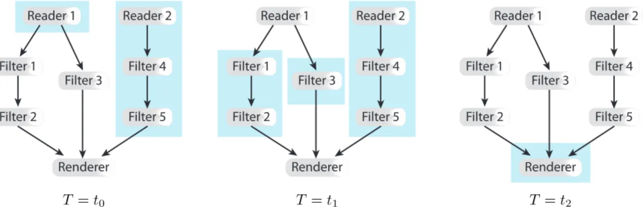
Task parallelism identifies independent portions of the pipeline and executes them concurrently. Independent parts of the pipeline occur where sources produce data indepen-dently or where fan out feeds multiple modules.
Fig. 4 demonstrates task parallelism applied to an exam-ple pipeline. At timet0the two readers begin executing
con-currently. Once the first reader completes, at timet1, both of
its downstream modules may begin executing concurrently. The other reader and its downstream modules may continue executing at this time, or they may sit idle if they have completed. (Fig. 4 implies that the Reader 2, Filter 4, Filter 5 subpipeline continues executing aftert1, which may or may
not be the actual case.) After all of its inputs complete, at timet2, the renderer executes.
Because task parallelism breaks a pipeline into indepen-dent sub-pipelines to execute concurrently, task parallelism can be applied to any type of algorithm. However, there are practical limits on how much concurrency can be achieved with task parallelism. Visualization pipelines in real working environments can seldom be broken into more than a hand-ful of independent sub-pipelines. Load balancing is also an issue. Concurrently running sub-pipelines are unlikely to finish simultaneously.
5.1.2 Pipeline Parallelism
Pipeline parallelismuses streaming to read data in pieces and executes different modules of the pipeline concurrently on different pieces of data. Pipeline parallelism is related to out-of-core processing in that a pipeline module is processing only a portion of the data at any one time, but in the pipeline-parallelism approach multiple pieces are loaded so that a module can process the next piece while downstream modules process the proceeding one.
Fig. 5 demonstrates pipeline parallelism applied to an example pipeline. At time t0 the reader loads the first piece
of data. At time t1, the loaded piece is passed to the filter
where it is processed while the second piece is loaded by the reader. Processing continues with each module working on the available piece while the upstream modules work on the next pieces.
Pipeline parallelism enables all the modules in the pipeline to be running concurrently. Thus, pipeline lelism tends to exhibit more concurrency than task paral-lelism, but the amount of concurrency is still severely limited by the number of modules in the pipeline, which is rarely much more than ten in practice. Load balancing is also an issue as different modules are seldom expected to finish in the same length of time. More compute intensive algorithms will stall the rest of the pipeline. Also, because pipeline parallelism is a form of streaming, it is limited to algorithms that are separable, result invariant, and mappable, as de-scribed in Section 3.5.
5.1.3 Data Parallelism
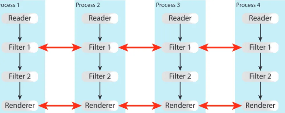
Data parallelism partitions the input data into some set number of pieces. It then replicates the pipeline for each
Process 1 Filter 1 Reader Filter 2 Renderer Process 3 Filter 1 Reader Filter 2 Renderer Process 4 Filter 1 Reader Filter 2 Renderer Process 2 Filter 1 Reader Filter 2 Renderer
Fig. 6: Concurrent execution with data parallelism. Boxes represent separate processes, each with its own partition of data. Communication among processes may also occur.
piece and executes them concurrently, as shown in Fig. 6. Of the three modes of concurrent scheduling, data paral-lelism is the most widely used. The amount of concurrency is limited only by the number of pieces the data can be split into, and for large-scale data that number is very high. Data parallelism also works well on distributed-memory parallel computers; data generally only needs to be partitioned once before processing begins. Data-parallel pipelines also tend to be well load balanced; identical algorithms running on equal sized inputs tend to complete in about the same amount of time.
Data parallelism is easiest to implement with algorithms that exhibit the separable, result invariant, and mappable criteria of streaming execution. In this case, the algorithm can be executed in data parallel mode with little if any change. However, it is possible to implement non-separable, non-result-invariant algorithms with data parallel execution. In this case, the data-parallel pipelines must allow com-munication among the processes executing a given module and the parallel executive must ensure that all pipelines get executed simultaneously lest the communication deadlock. Common examples of algorithms that have special data-parallel implementations are streamlines [53] and connected components [54]. Data-parallel pipelines also require special rendering for the partitioned data, which is described in the following section.
Data-parallel pipelines are shown to be very scalable. They have been successfully ported to current supercomput-ers [55], [56], [57] and have demonstrated excellent parallel speedup [58].
5.2 Rendering
Data parallel pipelines, particularly those running on distributed-memory parallel computers, require special con-sideration when rendering images, which is often the sink operation in a visualization pipeline. As in any part of the data parallel pipeline, the rendering module does not have complete access to the data. Rather, the data is partitioned among a number of replicated modules. In the case of rendering, this module’s processes must work together to form a single image from these distributed data.
A straightforward approach is to collect the data to a single process and render them serially [59], [60]. This collec-tion is sometimes feasible when rendering surfaces because
the surface geometry tends to be significantly smaller than the volumes from which it is derived. However, geometry for large-scale data can still exceed a single processor’s limits, and the approach is generally impractical for volume rendering techniques that require data for entire volumes. Thus, collecting data can become intractable.
A better approach is to employ a parallel rendering al-gorithm. Data-parallel pipelines are most often used with a class of parallel rendering algorithms called sort last [61]. Sort-last parallel rendering algorithms are characterized by each process first independently and concurrently rendering its local data into its own local image and then collectively reducing them into a single cohesive image.
Although it is possible to use other types of parallel rendering algorithms with visualization pipelines [62], the properties of sort-last algorithms make them most ideal for use in visualization pipelines. Sort-last rendering allows processes to render local data without concern about the partitioning (although there are caveats concerning transpar-ent objects [63]). Such behavior makes the rendering easy to adapt to whatever partition is created by the data-parallel pipeline. Also, the parallel overhead for sort-last rendering is independent of the amount of data being rendered, and sort last scales well with regard to the number of processes [64]. Thus, sort-last’s parallel scalability matches the parallel scal-ability of data-parallel pipelines.
5.3 Hybrid Parallel
Until recently, most high performance computers had dis-tributed nodes with each node containing some small amount of cores each. These computers could be effec-tively driven by treating each core as a distinct distributed-memory process.
However, that trend is changing. Current high perfor-mance computers now typically have 8–12 cores per node, and that number is expected to grow dramatically [65], [66], [67]. When this many cores are contained in a node, it is often more efficient to use hybrid parallelism that considers both the distributed memory parallelism among the nodes and the shared memory parallelism within each node [68]. Recent development shows that pipeline modules with hy-brid parallelism can out perform their corresponding mod-ules considering each core as a separate distributed memory node [69], [70], [71].
It should be noted that current implementations of hybrid parallelism are not a feature of the visualization pipeline. Rather, hybrid parallelism is implemented by creating mod-ules with algorithms that perform shared memory paral-lelism. The data-parallel pipeline then provides distributed memory parallelism on top of that.
6
E
MERGINGF
EATURESThis section describes emerging features of visualization pipelines that do not fit cleanly in any of the previous sections.
6.1 Provenance
Throughout this document we have considered the vi-sualization pipeline as a static construct that transforms data. However, in real visualization applications, the ex-ploratory process involves making changes to the visualiza-tion pipeline (i.e. adding and removing modules or making parameter changes). It is therefore possible to model explo-ration as transformations to the visualization pipeline [72]. Thisprovenanceof exploratory visualization can be captured and exploited.
Provenance of pipeline transformations can assist ex-ploratory visualization in many ways. Provenance allows users to quickly explore multiple visualization methods and compare various parameter changes [21]. It also assists in reproducibility; because provenance records the steps required to achieve a particular visualization, it can be saved to automate the same visualization later [73].
Provenance information engenders the rare ability to per-form analysis of analysis, which allows for powerful sup-porting abilities. Provenance information can be compared and combined to provide revisioning information for col-laborative analysis tasks [74]. Provenance information from previous analyses can be mined for future exploration. Such data can be queried for apropos visualization pipelines [75] or used to automatically assist users in their exploratory endeavors [76].
6.2 Scheduling on Heterogeneous Systems
Computer architecture is rapidly moving to heterogeneous architecture. GPU units with general-purpose computing capabilities are already common, and the use of similar accelerator units is likely to grow [65], [77].
Heterogeneous architectures introduce significant compli-cations when managing pipeline execution. The algorithms in different pipeline modules may need to run on different types of processors. If an algorithm is capable of running on different types of processors, it will have different perfor-mance characteristics on each one, which complicates load balancing.
Furthermore, heterogeneous architectures typically have a more complicated memory hierarchy. For example, a CPU and GPU on the same system usually have mutually inaccessible memory. Even when memory is shared, there is typically an affinityto some section of memory, meaning that data in some parts of memory can be accessed faster than data in other parts of memory. All this means that the pipeline execution must also consider data location.
Hyperflow [78] is an emerging technology to address these issues. Hyperflow manages parallel pipeline execution on heterogeneous systems. It combines all three modes of parallel execution (task, pipeline, and data described in Section 5.1) along with out-of-core streaming (described in Section 3.5) to dynamically allocate work based on thread availability and data location.
6.3 In Situ
In situ visualization refers to visualization that is run in tandem with the simulation that is generating the results being visualized. There are multiple approaches to in situ visualization. Some directly share memory space whereas others share data through high speed message passing. Nevertheless, all in situ visualization systems share two properties: the simulation and the visualization are run concurrently (or equivocally with appropriate time slices) and the passing of data from simulation to visualization bypasses the costly step of writing to or reading from a file on disk.
The concept of in situ visualization is as old as the field of visualization itself [1]. However, the interest in in situ visualization has grown significantly in recent years. Studies show that the cost of dedicated interactive visualization computers is increasing [79] and that the time spent in writing data to and reading data from disk storage is beginning to dominate the time spent in both the simulation and the visualization [80], [81], [82]. Consequently, in situ visualization is one of the most important research topics in large scale visualization today [67], [83].
In situ visualization does not involve visualization pipelines per se. In principle any visualization architecture can be coupled with a simulation. However, many cur-rent projects are using visualization pipelines for in situ visualization [60], [84], [85], [86], [87], [88] because of the visualization pipeline’s flexibility and the abundance of existing implementations.
7
V
ISUALIZATIONP
IPELINEA
LTERNATIVES Although visualization pipelines are the most widely used visualization framework, others exist and are being devel-oped today. This section contains a small sample of other visualization systems under current research and develop-ment.7.1 Functional Field Model
Most visualization systems represent fields as a data struc-ture directly storing the value for the field at each appro-priate place in the mesh. However, it is also possible to represent a field functionally. That is, provide a function that accepts a mesh location as its input argument and returns the field value for that location as its output. Functional fields are implemented in the Field Model (FM) library, a follow-on to the Field Encapsulation Library (FEL) [89].
A field function could be as simple as retrieving values from a data structure like that previously described, or it can abstract the data representation in many ways to simplify advanced visualization tasks. For example, the field function
could abstract the physical location of the data by paging it from disk as necessary [90].
Field functions also make it simple to definederived fields, that is fields computed from other fields. Functions for derived fields can be composed together to create something very much like the dataflow network of a visualization pipeline. The function composition, however, shares much of the behaviors of functional programming such as allow-ing for a lazy evaluation on a per-field-value basis [91].
The functional field model yields several advantages. It has a simple lazy evaluation model [91], it simplifies out-of-core paging [90], and it tends to have low overhead, which can simplify using it in situ with simulation [92]. However, unlike the visualization pipeline, the dataflow for composed fields are fixed in a demand-driven, or pull, execution model. Also, computation is limited to producing derived fields; there is no inherent mechanism to, for example, generate new topology.
7.2 MapReduce
MapReduce[93] is a cloud-based, data-parallel infrastructure designed to process massive amounts of data quickly. Al-though it was originally designed for performing distributed database search capabilities, many researchers and develop-ers have been successful at applying MapReduce to other problem domains and for more general-purpose program-ming [94], [95]. MapReduce garners much popularity due to its parallel scalability, its ability to run on inexpensive “share-nothing” parallel computers, and its simplified pro-gramming model.
As its name implies, the MapReduce framework runs programs in two phases: a map phase and a reduce phase. In the map phase, a user-provided function is applied independently and concurrently to all items in a set of data. Each instance of the map function returns one or more(key, value)pairs. In thereducephase, a user-provided function accepts all values with the same key and produces a result from them. Implicit in the framework is a shuffleof the(key, value)pairs in between the map and reduce phases. MapReduce’s versatility has enabled it to be applied to many scientific domains including visualization. It has been used to both process geometry [96] and render [96], [97]. The MapReduce framework allows visualization algorithms to be run in parallel in a much finer granularity than the parallel execution models of a visualization pipeline. However, the constraints imposed by MapReduce make it more difficult to design visualization algorithms, and there is no inherent way to combine algorithms such as can be done in a visualization pipeline.
7.3 Fine-Grained Data Parallelism
The data parallel execution model of visualization pipelines, described in Section 5.1.3, is scalable because it affords a large degree of concurrency. The amount of parallel threads is limited only by the number of partitions an input mesh can be split into. In theory, the input data can be split almost indefinitely, but in practice there are limits to how many parallel threads can be used for a particular mesh. Current implementations of parallel visualization pipelines
operate most efficiently with on the order of 100,000 to 1,000,000 cells per processing thread [29]. With fewer cells than that, each core tends to be bogged down with execution overhead, supporting structure, and boundary conditions. It is partly this reason that hybrid parallel pipelines, described in Section 5.3, perform better on multi-core nodes.
The problem with hybrid parallelism is that it is not a mechanism directly supported by the pipeline execution mechanics. Several projects seek to fill this gap by providing fine-grained algorithms designed to run on either GPU or multi-core CPU.
One project, PISTON [98], provides implementations of fine-grained data-parallel visualization algorithms. PISTON provides portability among multi- and many-core architec-tures by using basic parallel operations such as reductions, prefix sums, sorting, and gathering implemented on top of Thrust [99], a parallel template library, in such a way that they can be ported across multiple programming models.
Another project, Dax [100], provides higher level abstrac-tions for building fine-grained data-parallel visualization algorithms. Dax identifies common visualization operations, such as mapping a function to the local neighborhood of a mesh element or building geometry, and provides basic par-allel operations with fine-grained concurrency. Algorithms are built in Dax by providing worklets, serial functions that operate on a small region of data, and applying these worklets to the basic operations. The intention is to sim-plify visualization algorithm development while encourag-ing good data-parallel programmencourag-ing practices.
A third project, EAVL [101], provides an abstract data model that can be adapted to a variety of topological layouts. Operations on mesh elements and sub-elements are predicated by applying in parallelfunctors, structures acting like functions, on the elements of the mesh. These functors are easy-to-design serial components but can be scheduled on many concurrent threads.
7.4 Domain Specific Languages
Domain specific languages provide a new or augmented programming language with extended operations helpful for a specific domain of problems. Most visualization sys-tems are built as a library on top of a language rather than modify the language itself although there are some examples of domain specific languages that can insert visualization operations during a computer graphics rendering [102], [103].
Recently, domain specific languages emerged to build visualization on new highly threaded architectures. For example, Scout [104] functionally defines fields and oper-ations that can be executed on a GPU during visualization. Liszt [105] provides provides special language constructs for operations on unstructured grids. These operations are prin-cipally built to support partial differential equation solving but can also be used for analysis.
8
C
ONCLUSIONThe visualization community faces many challenges adapt-ing pipeline structures to future visualization needs, partic-ularly those associated with the push to exascale computing.
One primary challenge of exascale computing is the shift to massively threaded, heterogeneous, accelerator-based archi-tectures [67]. Although a visualization pipeline can support algorithms that drive such architectures (see the hybrid parallelism in Section 5.3), the execution models described in Section 5.1 are currently not generally scalable to the fine level of concurrency required. Most likely, independent design metaphors [98], [100], [101] will assist in algorithm design. Some of these current projects already have plans to encapsulate their algorithms in existing visualization pipeline implementations.
Another potential problem facing visualization pipelines and visualization applications in general is the memory usage. Predictions indicate that the cost of computation (in terms of operations per second) will decrease with respect to the cost of memory. Hence, we expect the amount of memory available for a particular problem size to decrease in future computer systems. Visualization algorithms are typically geared to provide a short computation on a large amount of data, which makes them favor “memory fat” computer nodes. Visualization pipelines often impose an extra memory overhead. Expect future work on making visualization pipelines leaner.
Finally, as simulations take advantage of increasing com-pute resources, they sometimes require new topological features to capture their complexity. Although the design of data structures is independent of the design of dataflow networks, dataflow networks like a visualization pipeline are difficult to dynamically adjust to data structures as the connections and operations are in part defined by the data structure. Consequently, visualization pipeline systems have been slow to adapt new data structures. Schroeder et al. [106] provide a generic, iterator-based interface to topology and field data that can be used within a visual-ization pipeline, but because its abstract interface hides the data layout and capabilities, result data cannot be written back into these structures. Thus, the first non-trivial module typically must tessellate the geometry into a form the native data structures can represent.
Regardless, the simplicity, versatility, and power of vi-sualization pipelines make them the most widely used framework for visualization systems today. These dataflow networks are likely to remain the dominant structure in visualization for years to come. It is therefore important to understand what they are, how they have evolved, and the current features they implement.
A
CKNOWLEDGMENTSThis work was supported in part by the DOE Office of Science, Advanced Scientific Computing Research, under award number 10-014707, program manager Lucy Nowell.
Sandia National Laboratories is a multi-program labo-ratory operated by Sandia Corporation, a wholly owned subsidiary of Lockheed Martin Corporation, for the U.S. Department of Energy’s National Nuclear Security Admin-istration.
R
EFERENCES[1] B. H. McCormick, T. A. DeFanti, and M. D. Brown, Eds.,Visualization in Scientific Computing (special issue of Computer Graphics). ACM, 1987, vol. 21, no. 6.
[2] P. E. Haeberli, “ConMan: A visual programming language for inter-active graphics,” inComputer Graphics (Proceedings of SIGGRAPH 88), vol. 22, no. 4, August 1988, pp. 103–111.
[3] B. Lucas, G. D. Abram, N. S. Collins, D. A. Epstein, D. L. Gresh, and K. P. McAuliffe, “An architecture for a scientific visualization system,” inIEEE Visualization, 1992, pp. 107–114.
[4] C. Upson, T. F. Jr., D. Kamins, D. Laidlaw, D. Schlegel, J. Vroom, R. Gurwitz, and A. van Dam, “The application visualization system: A computational environment for scientific visualization,”IEEE Com-puter Graphics and Applications, vol. 9, no. 4, pp. 30–42, July 1989. [5] D. D. Hils, “DataVis: A visual programming language for scientific
visualization,” inACM Annual Computer Science Conference (CSC ’91), March 1991, pp. 439–448, DOI 10.1145/327164.327331.
[6] D. S. Dyer, “A dataflow toolkit for visualization,”IEEE Computer Graphics and Applications, vol. 10, no. 4, pp. 60–69, July 1990. [7] D. Foulser, “IRIS Explorer: A framework for investigation,” in
Pro-ceedings of SIGGRAPH 1995, vol. 29, no. 2, May 1995, pp. 13–16. [8] W. Schroeder, W. Lorensen, G. Montanaro, and C. Volpe, “Visage:
An object-oriented scientific visualization system,” in Proceedings of Visualization ’92, October 1992, pp. 219–226, DOI 10.1109/VI-SUAL.1992.235205.
[9] G. Abram and L. A. Treinish, “An extended data-flow architecture for data analysis and visualization,” inProceedings of Visualization ’95, October 1995, pp. 263–270.
[10] S. G. Parker and C. R. Johnson, “SCIRun: A scientific programming environment for computational steering,” inProceedings ACM/IEEE Conference on Supercomputing, 1995.
[11] W. Schroeder, K. Martin, and B. Lorensen,The Visualization Toolkit: An Object Oriented Approach to 3D Graphics, 4th ed. Kitware Inc., 2004, ISBN 1-930934-19-X.
[12] M. Kass, “CONDOR: Constraint-based dataflow,” inComputer Graph-ics (Proceedings of SIGGRAPH 92), vol. 26, no. 2, July 1992, pp. 321–330. [13] G. D. Abram and T. Whitted, “Building block shaders,” inComputer Graphics (Proceedings of SIGGRAPH 90), vol. 24, no. 4, August 1990, pp. 283–288.
[14] R. L. Cook, “Shade trees,” inComputer Graphics (Proceedings of SIG-GRAPH 84), vol. 18, no. 3, July 1984, pp. 223–231.
[15] K. Perlin, “An image synthesizer,” inComputer Graphics (Proceedings of SIGGRAPH 85), no. 3, July 1985, pp. 287–296.
[16] D. Koelma and A. Smeulders, “A visual programming interface for an image processing environment,” Pattern Recognition Letters, vol. 15, no. 11, pp. 1099–1109, November 1994, DOI 10.1016/0167-8655(94)90125-2.
[17] C. S. Williams and J. R. Rasure, “A visual language for image pro-cessing,” inProceedings of the 1990 IEEE Workshop on Visual Languages, October 1990, pp. 86–91, DOI 10.1109/WVL.1990.128387.
[18] A. C. Wilson, “A picture’s worth a thousand lines of code,”Electronic System Design, pp. 57–60, July 1989.
[19] L. Ib´a ˜nez and W. Schroeder, The ITK Software Guide, ITK 2.4 ed. Kitware Inc., 2003, ISBN 1-930934-15-7.
[20] A. H. Squillacote, The ParaView Guide: A Parallel Visualization Application. Kitware Inc., 2007, ISBN 1-930934-21-1. [Online]. Available: http://www.paraview.org
[21] L. Bavoil, S. P. Callahan, P. J. Crossno, J. Freire, C. E. Scheidegger, C. T. Silva, and H. T. Vo, “VisTrails: Enabling interactive multiple-view visualizations,” inProceedings of IEEE Visualization, October 2005, pp. 135–142.
[22] P. Ramachandran and G. Varoquaux, “Mayavi: 3D visualization of scientific data,”Computing in Science & Engineering, vol. 13, no. 2, pp. 40–51, March/April 2011, DOI 10.1109/MCSE.2011.35.
[23] VisIt User’s Manual, Lawrence Livermore National Laboratory, Octo-ber 2005, technical Report UCRL-SM-220449.
[24] Kitware Inc., “VolView 3.2 user manual,” June 2009.
[25] A. Rosset, L. Spadola, and O. Ratib, “OsiriX: An open-source software for navigating in multidimensional dicom images,”Journal of Digital Imaging, vol. 17, no. 3, pp. 205–216, September 2004.
[26] S. Pieper, M. Halle, and R. Kikinis, “3D slicer,” inProceedings of the 1st IEEE International Symposium on Biomedical Imaging: From Nano to Macro 2004, April 2004, pp. 632–635.
[27] P. Kankaanp¨a¨a, K. Pahajoki, V. Marjom¨aki, D. White, and J. Heino, “BioImageXD - free microscopy image processing software,” Mi-croscopy and Microanalysis, vol. 14, no. Supplement 2, pp. 724–725, August 2008.
[28] W. E. Lorensen and H. E. Cline, “Marching cubes: A high resolution 3D surface construction algorithm,”Computer Graphics (Proceedings of SIGGRAPH 87), vol. 21, no. 4, pp. 163–169, July 1987.
[29] K. Moreland, “The paraview tutorial, version 3.10,” Sandia National Laboratories, Tech. Rep. SAND 2011-4481P, 2011.
[30] SCIRun Development Team,SCIRun User Guide, Center for Integra-tive Biomedical Computing, University of Utah.
[31] IRIS Explorer User’s Guide, The Numerical Algorithms Group Ltd., 2000, ISBN 1-85206-190-1, NP3520.
[32] VisTrails Documentation, University of Utah, April 2011.
[33] D. Thompson, J. Braun, and R. Ford,OpenDX: Paths to Visualization. VIS Inc., 2001.
[34] H. T. Vo, D. K. Osmari, B. Summa, J. L. D. Comba, V. Pascucci, and C. T. Silva, “Streaming-enabled parallel dataflow architecture for multicore systems,”Computer Graphics Forum (Proceedings of EuroVis 2010), vol. 29, no. 3, pp. 1073–1082, June 2010.
[35] K. Inc., The VTK User’s Guide, 11th ed. Kitware Inc., 2010, ISBN 978-1-930934-23-8.
[36] J. S. Vitter, “External memory algorithms and data structures: Dealing with massive data,”AVM Computing Surveys, vol. 33, no. 2, June 2001. [37] C. C. Law, K. M. Martin, W. J. Schroeder, and J. Temkin, “A multi-threaded streaming pipeline architecture for large structured data sets,” inProceedings of IEEE Visualization 1999, October 1999, pp. 225– 232.
[38] J. Ahrens, K. Brislawn, K. Martin, B. Geveci, C. C. Law, and M. Papka, “Large-scale data visualization using parallel data stream-ing,”IEEE Computer Graphics and Applications, vol. 21, no. 4, pp. 34–41, July/August 2001.
[39] M. J. Berger and P. Colella, “Local adaptive mesh refinement for shock hydrodynamics,”Journal of Computational Physics, vol. 82, no. 1, pp. 64–84, May 1989.
[40] J. Biddiscombe, B. Geveci, K. Martin, K. Moreland, and D. Thomp-son, “Time dependent processing in a parallel pipeline archi-tecture,” IEEE Transactions on Visualization and Computer Graph-ics, vol. 13, no. 6, pp. 1376–1383, November/December 2007, DOI 10.1109/TVCG.2007.70600.
[41] H. Childs, E. Brugger, K. Bonnell, J. Meredith, M. Miller, B. Whitlock, and N. Max, “A contract based system for large data visualization,” inIEEE Visualization 2005, 2005, pp. 191–198.
[42] J. P. Ahrens, N. Desai, P. S. McCormic, K. Martin, and J. Woodring, “A modular, extensible visualization system architecture for culled, prioritized data streaming,” inVisualization and Data Analysis 2007, 2007, pp. 64 950I:1–12.
[43] J. P. Ahrens, J. Woodring, D. E. DeMarle, J. Patchett, and M. Mal-trud, “Interactive remote large-scale data visualization via prioritized multi-resolution streaming,” inProceedings of the 2009 Ultrascale Vi-sualization Workshop, November 2009, DOI 10.1145/1838544.1838545. [44] K. Stockinger, J. Shalf, K. Wu, and E. W. Bethel, “Query-driven visualization of large data sets,” in Proceedings of IEEE Visualization 2005, October 2005, pp. 167–174.
[45] L. J. Gosink, J. C. Anderson, E. W. Bethel, and K. I. Joy, “Query-driven visualization of time-varying adaptive mesh refinement data,”IEEE Transactions of Visualization and Computer Graphics, vol. 14, no. 6, pp. 1715–1722, November/December 2008.
[46] Y.-J. Chiang, C. T. Silva, and W. J. Schroeder, “Interactive out-of-core isosurface extraction,” inProceedings of IEEE Visualization ’98, October 1998, pp. 167–174.
[47] K. Wu, S. Ahern, E. W. Bethel, J. Chen, H. Childs, E. Cormier-Michel, C. Geddes, J. Gu, H. Hagen, B. Hamann, W. Koegler, J. Lauret, J. Meredith, P. Messmer, E. Otoo, V. Perevoztchikov, A. Poskanzer, Prabhat, O. R ¨ubel, A. Shoshani, A. Sim, K. Stockinger, G. We-ber, and W.-M. Zhang, “FastBit: interactively searching massive data,”Journal of Physics: Conference Series, vol. 180, p. 012053, 2009, DOI 10.1088/1742-6596/180/1/012053.
[48] K. Wu, A. Shoshani, and K. Stockinger, “Analyses of multi-level and multi-component compressed bitmap indexes,”ACM Transactions on Database Systems (TODS), vol. 35, p. Article 2, February 2010. [49] M. Glatter, J. Huang, S. Ahern, J. Daniel, and A. Lu, “Visualizing
temporal patterns in large multivariate data using textual pattern matching,”IEEE Transactions of Visualization and Computer Graphics, vol. 14, no. 6, pp. 1467–1474, November/December 2008.
[50] C. R. Johnson and J. Huang, “Distribution-driven visualization of vol-ume data,” IEEE Transactions of Visualization and Computer Graphics, vol. 15, no. 5, September/October 2009.
[51] O. R ¨ubel, Prabhat, K. Wu, H. Childs, J. Meredith, C. G. Geddes, E. Cormier-Michel, S. Ahern, G. H. Weber, P. Messmer, H. Hagen, B. Hamann, and E. W. Bethel, “High performance multivariate visual data exploration for extremely large data,” inProceedings of the 2008 ACM/IEEE Conference on Supercomputing, November 2008.
[52] J. Ahrens, C. Law, W. Schroeder, K. Martin, and M. Papka, “A parallel approach for efficiently visualizing extremely large, time-varying datasets,” Los Alamos National Laboratory, Tech. Rep. #LAUR-00-1620, 2000.
[53] D. Pugmire, H. Childs, C. Garth, S. Ahern, and G. Weber, “Scalable computation of streamlines on very large datasets,” inProceedings of ACM/IEEE Conference on Supercomputing, November 2009.
[54] K. Moreland, C. C. Law, L. Ice, and D. Karelitz, “Analysis of frag-mentation in shock physics simulation,” in Proceedings of the 2008 Workshop on Ultrascale Visualization, November 2008, pp. 40–46. [55] K. Moreland, D. Rogers, J. Greenfield, B. Geveci, P. Marion, A.
Ne-undorf, and K. Eschenberg, “Large scale visualization on the Cray XT3 using paraview,” inCray User Group, 2008.
[56] D. Pugmire, H. Childs, and S. Ahern, “Parallel analysis and visual-ization on cray compute node linux,” inCray User Group, 2008. [57] J. Patchett, J. Ahrens, S. Ahern, and D. Pugmire, “Parallel
visualiza-tion and analysis with ParaView on a Cray Xt4,” inCray User Group, 2009.
[58] H. Childs, D. Pugmire, S. Ahern, B. Whitlock, M. Howison, Prabhat, G. H. Weber, and E. W. Bethel, “Extreme scaling of production visu-alization software on diverse architectures,”IEEE Computer Graphics and Applications, pp. 22–31, May/June 2010.
[59] M. Miller, C. D. Hansen, S. G. Parker, and C. R. Johnson, “Simulation steering with SCIRun in a distributed memory environment,” in Applied Parallel Computing Large Scale Scientific and Industrial Problems, ser. Lecture Notes in Computer Science, vol. 1541, 1998, pp. 366–376, DOI 10.1007/BFb0095358.
[60] C. Johnson, S. G. Parker, C. Hansen, G. L. Kindlmann, and Y. Livnat, “Interactive simulation and visualization,”IEEE Computer, vol. 32, no. 12, pp. 59–65, December 1999, DOI 10.1109/2.809252.
[61] S. Molnar, M. Cox, D. Ellsworth, and H. Fuchs, “A sorting classifica-tion of parallel rendering,”IEEE Computer Graphics and Applications, vol. 14, no. 4, pp. 23–32, July 1994.
[62] K. Moreland and D. Thompson, “From cluster to wall with VTK,” in Proceedings of IEEE Symposium on Parallel and Large-Data Visualization and Graphics, October 2003, pp. 25–31.
[63] K. Moreland, L. Avila, and L. A. Fisk, “Parallel unstructured volume rendering in paraview,” inVisualization and Data Analysis 2007, Pro-ceedings of SPIE-IS&T Electronic Imaging, January 2007, pp. 64 950F– 1–12.
[64] B. Wylie, C. Pavlakos, V. Lewis, and K. Moreland, “Scalable rendering on PC clusters,”IEEE Computer Graphics and Applications, vol. 21, no. 4, pp. 62–70, July/August 2001.
[65] J. Dongarra, P. Beechmanet al., “The international exascale software project roadmap,” University of Tennessee, Tech. Rep. ut-cs-10-652, January 2010. [Online]. Available: http://www.cs.utk.edu/∼library/ TechReports/2010/ut-cs-10-652.pdf
[66] S. Ashbyet al., “The opportunities and challenges of exascale com-puting,” Summary Report of the Advanced Scientific Computing Advisory Committee (ASCAC) Subcommittee, Fall 2010.
[67] S. Ahern, A. Shoshani, K.-L. Maet al., “Scientific discovery at the exascale,” Report from the DOE ASCR 2011 Workshop on Exascale Data Management, Analysis, and Visualization, February 2011. [68] F. Cappello and D. Etiemble, “MPI versus MPI+OpenMP on the IBM
SP for the NAS benchmarks,” inProceedings of the 2000 ACM/IEEE Conference on Supercomputing, November 2000.
[69] L. Chen and I. Fujishiro, “Optimization strategies using hybrid MPI+OpenMP parallelization for large-scale data visualization on earth simulator,” inA Practical Programming Model for the Multi-Core Era. Springer, 2008, vol. 4935, pp. 112–124, DOI 10.1007/978-3-540-69303-1 10.
[70] D. Camp, C. Garth, H. Childs, D. Pugmire, and K. Joy, “Stream-line integration using MPI-hybrid parallelism on large multi-core architecture,”IEEE Transactions on Visualization and Computer Graphics, December 2010, DOI 10.1109/TVCG.2010.259.
[71] M. Howison, E. W. Bethel, and H. Childs, “Hybrid parallelism for volume rendering on large, multi- and many-core systems,” IEEE Transactions on Visualization and Computer Graphics, January 2011, DOI 10.1109/TVCG.2011.24.
[72] T. Jankun-Kelly, K.-L. Ma, and M. Gertz, “A model for the visual-ization exploration process,” inProceedings of IEEE Visualization 2002, October 2002, pp. 323–330.
[73] C. T. Silva, J. Freire, and S. P. Callahan, “Provenance for visu-alizations: Reproducibility and beyond,” Computing in Science & Engineering, vol. 9, no. 5, pp. 82–89, September/October 2007, DOI 10.1109/MCSE.2007.106.
[74] T. Ellkvist, D. Koop, E. W. Anderson, J. Freire, and C. Silva, “Using provenance to support real-time collaborative design of workflows,” inProceedings of the International Provenance and Annotation Workshop,
ser. Lecture Notes in Computer Science, vol. 5272. Springer, 2008, pp. 266–279, DOI 10.1007/978-3-540-89965-5 27.
[75] C. E. Scheidegger, H. T. Vo, D. Koop, J. Freire, and C. T. Silva, “Querying and creating visualizations by analogy,” Querying and Creating Visualizations by Analogy, vol. 13, no. 6, pp. 1560–1567, November/December 2007.
[76] D. Koop, C. E. Scheidegger, S. P. Callahan, J. Freire, and C. T. Silva, “VisComplete: Automating suggestions for visualization pipelines,” IEEE Transactions on Visualization and Computer Graphics, vol. 14, no. 6, pp. 1691–1698, November/December 2008.
[77] R. Stevens, A. Whiteet al., “Architectures and technology for extreme scale computing,” ASCR Scientific Grand Challenges Workshop Se-ries, Tech. Rep., December 2009.
[78] H. T. Vo, “Designing a parallel dataflow architecture for streaming large-scale visualization on heterogeneous platforms,” Ph.D. disser-tation, University of Utah, May 2011.
[79] H. Childs, “Architectural challenges and solutions for petascale post-processing,” Journal of Physics: Conference Series, vol. 78, no. 012012, 2007, DOI 10.1088/1742-6596/78/1/012012.
[80] R. B. Ross, T. Peterka, H.-W. Shen, Y. Hong, K.-L. Ma, H. Yu, and K. Moreland, “Visualization and parallel I/O at extreme scale,” Journal of Physics: Conference Series, vol. 125, no. 012099, 2008, DOI 10.1088/1742-6596/125/1/012099.
[81] T. Peterka, H. Yu, R. Ross, and K.-L. Ma, “Parallel volume rendering on the IBM Blue Gene/P,” in Proceedings of Eurographics Parallel Graphics and Visualization Symposium 2008, 2008.
[82] T. Peterka, H. Yu, R. Ross, K.-L. Ma, and R. Latham, “End-to-end study of parallel volume rendering on the ibm blue gene/p,” in Proceedings of ICPP ’09, September 2009, pp. 566–573, DOI 10.1109/ICPP.2009.27.
[83] C. Johnson, R. Rosset al., “Visualization and knowledge discovery,” Report from the DOE/ASCR Workshop on Visual Analysis and Data Exploration at Extreme Scale, October 2007.
[84] J. Biddiscombe, J. Soumagne, G. Oger, D. Guibert, and J.-G. Piccinali, “Parallel computational steering and analysis for hpc applications using a paraview interface and the hdf5 dsm virtual file driver,” in Eurographics Symposium on Parallel Graphics and Visualization, 2011, pp. 91–100, DOI 10.2312/EGPGV/EGPGV11/091-100.
[85] N. Fabian, K. Moreland, D. Thompson, A. C. Bauer, P. Mar-ion, B. Geveci, M. Rasquin, and K. E. Jansen, “The ParaView coprocessing library: A scalable, general purpose in situ visual-ization library,” in Proceedings of the IEEE Symposium on Large-Scale Data Analysis and Visualization, October 2011, pp. 89–96, DOI 10.1109/LDAV.2011.6092322.
[86] S. Klaskyet al., “In situ data processing for extreme scale computing,” inProceedings of SciDAC 2011, July 2011.
[87] K. Moreland, R. Oldfield, P. Marion, S. Jourdain, N. Podhorszki, V. Vishwanath, N. Fabian, C. Docan, M. Parashar, M. Hereld, M. E. Papka, and S. Klasky, “Examples ofin transitvisualization,” in Petas-cale Data Analytics: Challenges and Opportunities (PDAC-11), November 2011.
[88] B. Whitlock, “Getting data into VisIt,” Lawrence Livermore National Laboratory, Tech. Rep. LLNL-SM-446033, July 2010.
[89] S. Bryson, D. Kenwright, and M. Gerald-Yamasaki, “FEL: The field encapsulation library,” inProceedings Visualization ’96, October 1996, pp. 241–247.
[90] M. Cox and D. Ellsworth, “Application-controlled demand paging for out-of-core visualization,” inProceedings Visualization ’97, October 1997, pp. 235–244, DOI 10.1109/VISUAL.1997.663888.
[91] P. J. Moran and C. Henze, “Large field visualization with demand-driven calculation,” inProceedings Visualization ’99, October 1999, pp. 27–33, DOI 10.1109/VISUAL.1999.809864.
[92] D. Ellsworth, C. Henze, B. Green, P. Moran, and T. Sand-strom, “Concurrent visualization in a production supercomputer environment,” IEEE Transactions on Visualization and Computer Graphics, vol. 12, no. 5, pp. 997–1004, September/October 2006, DOI 10.1109/TVCG.2006.128.
[93] J. Dean and S. Ghemawat, “MapReduce: Simplified data processing on large clusters,” Communications of the ACM, vol. 51, no. 1, pp. 107–113, January 2008.
[94] C. Olston, B. Reed, U. Srivastava, R. Kumar, and A. Tomkins, “Pig latin: A not-so-foreign language for data processing,” inProceedings of the 2008 ACM SIGMOD International Conference on Management of Data, 2008, DOI 10.1145/1376616.1376726.
[95] M. Isard and Y. Yu, “Distributed data-parallel computing using a high-level programming language,” in Proceedings of the 35th SIGMOD International Conference on Management of Data, 2009, DOI 10.1145/1559845.1559962.
[96] H. T. Vo, J. Bronson, B. Summa, J. L. Comba, J. Freire, B. Howe, V. Pascucci, and C. T. Silva, “Parallel visualization on large clus-ters using MapReduce,” in Proceedings of the IEEE Symposium on Large-Scale Data Analysis and Visualization, October 2011, pp. 81–88, DOI 10.1109/LDAV.2011.6092321.
[97] J. A. Stuart, C.-K. Chen, K.-L. Ma, and J. D. Owens, “Multi-GPU volume rendering using MapReduce,” in1st International Workshop on MapReduce and its Applications, June 2010.
[98] L.-T. Lo, C. Sewell, and J. Ahrens, “PISTON: A portable cross-platform framework for data-parallel visualization operators,” Los Alamos National Laboratory, LA-UR-11-11689, http://viz.lanl.gov/projects/PISTON.html.
[99] N. Bell and J. Hoberock,GPU Computing Gems, Jade Edition. Mor-gan Kaufmann, October 2011, ch. Thrust: A Productivity-Oriented Library for CUDA, pp. 359–371.
[100] K. Moreland, U. Ayachit, B. Geveci, and K.-L. Ma, “Dax toolkit: A proposed framework for data analysis and visualization at extreme scale,” in Proceedings of the IEEE Symposium on Large-Scale Data Analysis and Visualization, October 2011, pp. 97–104, DOI 10.1109/LDAV.2011.6092323.
[101] J. S. Meredith, R. Sisneros, D. Pugmire, and S. Ahern, “A distributed data-parallel framework for analysis and visualization algorithm development,” inProceedings of the 5th Annual Workshop on General Purpose Processing with Graphics Processing Units (GPGPU-5), March 2012, pp. 11–19, DOI 10.1145/2159430.2159432.
[102] B. Corrie and P. Mackerras, “Data shaders,” inProceedings of Visual-ization ’93, October 1993.
[103] R. A. Crawfis and M. J. Allison, “A scientific visualization synthe-sizer,” inProceedings of Visualization ’91, October 1991, pp. 262–267, DOI 10.1109/VISUAL.1991.175811.
[104] P. McCormick, J. Inman, J. Ahrens, J. Mohd-Yusof, G. Roth, and S. Cummins, “Scout: A data parallel programming environment for graphics processors,”Parallel Computing, vol. 33, no. 10–11, pp. 648– 662, November 2007.
[105] Z. DeVito, N. Joubert, F. Palacios, S. Oakley, M. Medina, M. Barrien-tos, E. Elsen, F. Ham, A. Aiken, K. Duraisamy, E. Darve, J. Alonso, and P. Hanrahan, “Liszt: A domain specific language for building portable mesh-based PDE solvers,” inProceedings of 2011 International Conference for High Performance Computing, Networking, Storage and Analysis (SC ’11), November 2011.
[106] W. J. Schroeder, F. Bertel, M. Malaterre, D. Thompson, P. P. P´ebay, R. O’Bara, and S. Tendulkar, “Methods and framework for visualizing higher-order finite elements,”IEEE Transactions on Visualization and Computer Graphics, vol. 12, no. 4, pp. 446–460, July/August 2006, DOI 10.1109/TVCG.2006.74.
Kenneth Morelandreceived the BS degrees in com-puter science and in electrical engineering from the New Mexico Institute of Mining and Technology in 1997. He received the MS and PhD degrees in computer science from the University of New Mexico in 2000 and 2004, respectively, and currently re-sides at Sandia National Laboratories. Dr. Moreland specializes in large-scale visualization and graphics and has played an active role in the development of ParaView, a general-purpose scientific visualization system capable of scalable parallel data processing. His current interests include the design and development of visualization al-gorithms and systems to run on multi-core, many-core, and future-generation computer hardware.