Control Flow Graph Transformations for
Exploiting Subword Parallelism in PET
Image Reconstruction
Bjorn De Sutter, Mark Christiaens
Department of Electronics and Information Systems University of Gent, Belgium
{brdsutte,mchristi}@elis.rug.ac.be
Abstract
Subword parallelism is a recent form of internal processor parallelism. In this article, we show how it can be used for non-multimedia applications. We optimized a Positron Emission Tomography image reconstruction us-ing the VISual Instruction Set on Sun’s UltraSPARC [Sun95] processor. Various control flow transformations are necessary to uncover possibili-ties to use subword parallelism, such as loop unrolling, loop fusion and if-hoisting. The speed-up we achieved by using subword parallelism is about 45%.
1
Introduction to Subword Parallelism
Subword parallelism (SP) is a recent form of internal processor parallelism. It was introduced with the rise of multimedia-extensions during the last two years. Multimedia-extensions are extensions to computer architectures to
Figure 1: Above an ordinary addition, below an SP addition
provide a faster way to operate on typical multimedia data. This data dif-fers from the data upon which general-purpose architectures operate mostly. Namely, multimedia data often has a width of 8 (video) or 16 (audio) bits, while the width of registers in modern architectures is 32 or 64 bits. Using only 8 or 16 of the available 32 or 64 bits waists a considerable amount of capacity.
A solution to alleviate this, is to pack multiple multimedia data elements (called subwords) in one register or word and operate on these subwords in parallel. This can be done easily by ordinary RISC-instructions with simple semantics, fixed length, etc.
The hardware implementation of SP is not difficult. In Figure 1 an ordinary addition of decimal data is compared with an SP addition. Note that the only difference in performing these operations is the lack of a carry between two subwords in the SP-addition. Figures from Hewlett-Packard, Intel and Sun indicate that less than 3% of the die area of their chips is spent on the MAX-2 [Lee96], MMX [Int96] or VISual Instruction Set [Sunil], their resp. multimedia-extensions.
The use of SP in a program is not trivial [Ric96]. To group operations into SP instructions, these operations have to be available in basic blocks. There-fore, SP can only be used if there are basic blocks containing several identical operations on independent data. Control flow transformations might be nec-essary to build these basic blocks in a program as to uncover the possibilities to use SP.
We will show this in section 5 for an algorithm used in PET image recon-struction. First we will introduce this medical imaging technique and its core functionality.
2
Positron Emission Tomography
Positron Emission Tomography (PET) is a medical technique that visualizes the metabolic activity in a section (2D) or volume (3D) in a patient’s body. For this purpose, a radioactive tracer is injected in the patient. The positrons in this tracer annihilate with electrons in the patient’s body, a process during which two photons are emitted in opposite directions.
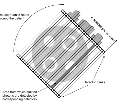
Since the tracer concentrates in parts of the body with higher metabolic activity, visualizing the number of emitted photons and thus the number of annihilations allows us to build an image of the metabolic activity inside the patient. For the sake of clarity, we will limit this discussion to the 2D case. The emitted photon pairs are detected by two detector banks around the patient, as depicted in Figure 2. Each detector pair only detects the photon pairs emitted in the beam between the two detectors. This is a simple as-sumption, but data transformations performed by the scanner make it a valid one. The data acquired, as shown in Figure 2 are not enough to reconstruct the section of the patient’s body. Therefore measurements are taken under different angels. The resulting data is visualized in Figure 3.
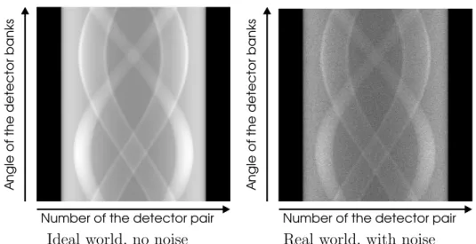
The left part of the figure shows what the data would look like in an ideal world, i.e. without noise. Unfortunately noise is introduced in the detection process for several reasons. It would lead us to far to delve any deeper in this, but it is important because noise is the reason the acquired data looks more like the right part of Figure 3. It is also the cause of artefacts in the constructed images if simple analytic methods are used for the reconstruction. Instead, we need iterative or statistical reconstruction algorithms. Maximum Likelihood-Expectation Maximization is such a statistical algorithm.
3
Maximum Likelihood - Expectation
Maxi-mization
Maximum Likelihood - Expectation Maximization (ML-EM) [SV82] is a sta-tistical reconstruction algorithm. It is named ML because we want to opti-mize the probability that the reconstructed image would produce the mea-sured data. EM is added to the name, since we use this iterative optimization method to find the ML solution of the problem. The statistical model used is as follows.
Number of the detector pair
A
ngle of the detector banks
Number of the detector pair
A
ngle of the detector banks
Ideal world, no noise Real world, with noise
Figure 3: Visualization of the measured data: each pixel density corresponds to a number of detected photons. The pixels of a line correspond to the detector pairs of a bank. There is such a line for each angle at which data is acquired.
body can be modeled as a Poisson process. Therefore the number of photons emitted in a pixel can be modeled as a Poisson process, where the aver-age number of photons emitted during an interval corresponds to the pixel density.
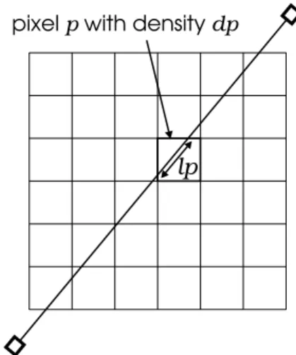
Using this as an underlying model, we now have to model the probability that a photon pair emitted in a pixel is detected by a certain detector pair. A very precise measure for this probability is the area in the pixel under the beam between the detectors of the detector pair. But since the calculation of this area is far too time-consuming, other measures have to be considered. It is shown that a good compromise between calculation speed and precision is the distance the ray connecting the detectors traverses in the pixel. Using this distance, the number of photons detected in a detector pair can be modeled as
RPdetector pair = X
all pixelsp
dp×lp, (1)
where dp is the density of pixel p and lp is the distance traversed in it (see Figure 4). This model is called the radiological path (RP).
lp
pixel pwith density dp
Figure 4: Definition of the radiological path
4
Radiological Paths
The calculation of RPs is performed millions of times during an image recon-struction: for each EM iteration, it is calculated for each ray at each angle. The distances lp have to be calculated on-the-fly, since to much memory is needed to store them permanently.
Until recently, the fastest algorithm known to calculate the RP was that by Siddon [Sid85]. We have proposed a new, faster algorithm, called the incremental algorithm. For the sake of brevity, we will explain in this article only the bare minimum necessary to understand the applicability of SP to this problem. For an in-depth description see [CDSDB+98].
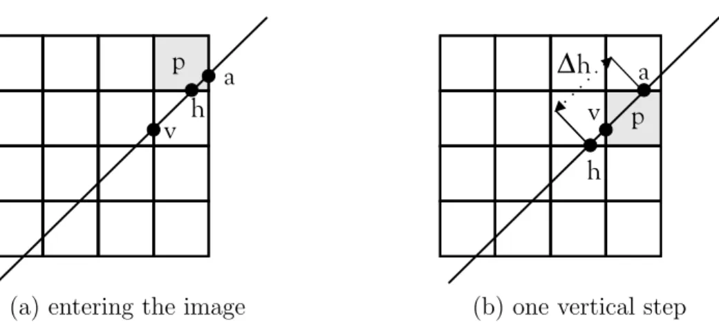
The ray is represented by a parameter varying linearly (see Figure 5a). First, we determine a, the parameter value of the entry point of the line into the image and the corresponding entry pixel p. Next, the first intersections of the line with horizontal or vertical pixel boundaries inside the image are calculated (with resp. parameter values h and v). This provides us with a basis to start calculating the RP.
Suppose that the pixel boundary through which we leave p is a horizontal one. This can easily be detected by noticing that h ≤ v. The measure for the length of the line segment in pis l =h−a. We obtain the contribution of pixel pto the RP by multiplying l with the density of p.
∆
(a) entering the image (b) one vertical step Figure 5: The parameter values during traversal of the image.
Figure 5b). The entry point into the next pixel is easily determined: it is the intersection with the horizontal line of which we already know the parameter value h. So we give a the value of h. The value of v need not change; the next intersection with a vertical line is still the same. We do, however, need to change the value of h. The new value ofh becomes h+ ∆h, where ∆h is the constant distance between two consecutive intersections with horizontal boundaries. Finally, after a simple integer addition, the new p points to the pixel under the previous one.
The calculations, as described in the previous paragraphs, are repeated until the line leaves the image. The total sum of all the contributions of the pixels forms the RP of the line.
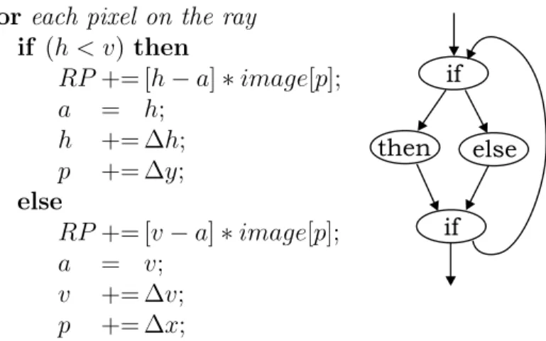
All this makes for a fairly simple iteration scheme, of which the code is shown in Figure 6. It has a few shortcomings however. First, for every pixel, we need to determine whether the line crossed a horizontal or vertical boundary. This results in a loop with an if-then-elseconstruct inside the inner loop producing code with small basic blocks. Second, every iteration is dependent on the previous one, making the use of SP nontrivial.
5
Control Flow Transformations
First of all, we can see that the iterations of the inner loop are not in-dependent. A way in which we can achieve an inner loop with identical, independent operations is by computing the RP for several rays in lock-step.
for each pixel on the ray if (h < v) then RP+= [h−a]∗image[p]; a = h; h += ∆h; p += ∆y; else RP+= [v−a]∗image[p]; a = v; v += ∆v; p += ∆x;
Figure 6: Pseudo-code and CFG for the inner loop in the RP calculation
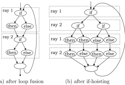
Since the RP is calculated for numerous parallel rays, with a loop over these parallel rays, we can unroll this loop. Using software pipelining, we can put the nested loops of the RP-calculations for different rays after each other. These consecutive inner loops can then be fused to create one inner loop. The result of these transformations is shown in Figure 7a. In the upper part of the loop body, a step for the first ray is taken, in the lower part the same is done for ray 2. Note that these parts are completely independent from each other. (Off course, variables are renamed in both parts.) As can be seen in Figure 6 the then and else parts of the CFG are identical with respect to the operations they perform. Thus, merging these blocks in one way or another uncovers SP.
A transformation that results in the merged basic blocks is if-hoisting. Since the calculations for the two rays are independent, the order in which they are performed does not matter. The if-test of the lower part can be hoisted, but then we have to duplicate the then and else part of the upper part. The resulting CFG is shown in Figure 7b.
It is clear that the consecutive basic blocks in the lower half of the inner loop body can be merged together. Since they contain identical operations on independent data (ray 1 vs. ray 2), they are fit for exploiting SP.
(a) after loop fusion (b) after if-hoisting
Figure 7: Control flow graph of the inner loop in the calculation of a RP for 2 rays
6
Exploiting Subword Parallelism
In this section, we will show how we exploited SP on Sun’s UltraSPARC processor. This processor implements the SPARCv9 architecture [SI94], in-cluding the VISual Instruction Set, Sun’s multimedia-extensions.
Though we will use the single unrolled loop in the figures for clarity, we have unrolled the loop over parallel rays 4-fold. This way, the RPs of 4 rays are calculated in lock-step.
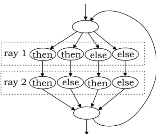
A first thing that can be optimized is the tree of if-tests. Note that the same if-tests are performed on each of the 16 (24) paths in the inner loop body. Since these tests are simple comparisons, they can be performed in parallel. The result on the UltraSPARC architecture is a 4 bit bit-field (one bit for each comparison), which can be used as an index in a jump table. This way, after 1 table look-up, we can jump directly to the correct combination of
then and else parts. The resulting CFG is depicted in Figure 8.
Next, we can use SP in the merged then and else blocks. The conversion to SP operations implies more than the replacement of several identical in-structions by a parallel one. The operands of the original inin-structions have to be packed in words and become subwords before one can operate on them in parallel. Three steps are necessary in general.
Figure 8: The control flow graph, using a parallel comparison
Packing data in registers In our algorithm,a-values,h-values andv-values for each of the 4 lines are grouped in hai, hhi and hvi. This grouping is fixed for the whole execution of the loop.
Loading data elements In each iteration, 4 new pixel values are loaded. These are loaded separately, each in a different register. We need to pack them into one register in each iteration. This is the main differ-ence between our type of algorithm and typical imaging or multimedia applications. In those applications, operations on data streams run through the data in a very regular form in which adjacent pixels can be loaded in parallel and can be operated upon immediately. We need more preparatory work to pack the data elements in registers.
Performing operations In every iteration some of the elements of hhiare updated (then-part in the original program), as well as other elements inhvi(else-part in the original program). Operations to some elements in hhi can be performed using masks.
For example, an addition to the first and third subword of hhi is done by adding h∆hi to it, where the second and fourth element of h∆hi
are set to zero by a mask. The use of masks is straightforward, but to be efficient, enough registers have to be available. In our program, 16 different masks are used, which are best placed in registers permanently. Summarizing, we can say that variables used in the loop have to be packed,
masks have to be used to perform the correct operations and pixels have to be loaded en merged in registers.
It is important to note that the calculation of pixel indices is not done using SP. These calculations are done using integer arithmetic and thus are exe-cuted in parallel with the SP operations on superscalar architectures. Besides that, for large images, the range needed for the indices would be too large to fit in subwords anyway.
7
Results
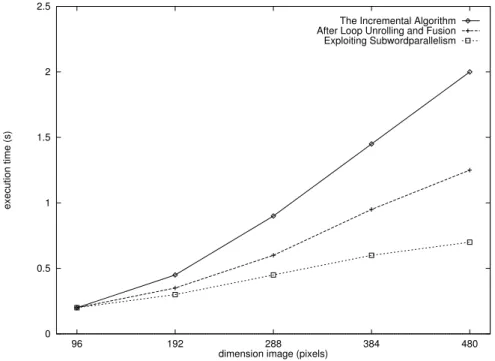
Having described how and by what means the incremental algorithm is im-plemented to exploit SP, we can now give results of these optimizations. In Figure 9 the execution times for a PET image reconstruction are plotted for various image sizes.
We embedded our routines in an existing 2D PET reconstruction program, emvox2d.1 This program uses the ML-EM algorithm [SV82], in which RP calculations take about 90% of the time. Our algorithm is linear in the sum of the dimensions of the image. Any non-linearities in the graph result from cache-behavior.
The speed-up achieved by exploiting SP is 45% compared to our best C-code optimized using the SCO 4.0 compiler. This is not only due to the use of subword parallelism, but also to the better cache behavior: the pixels are represented in a smaller data format and thus more pixels fit in the cache. Finally, it is noteworthy to say that our optimizations are applicable to 3D PET image reconstruction as well.
8
Acknowledgement
We would like to thank Jan Van Campenhout and Koen De Bosschere, our promotor and adviser for our graduation thesis, of which this article is a re-sult. Our thanks go to Erik D’Hollander as well for the excellent organisation of this seminar in Gent.
1This evaluation program is developed by the Medical Image Processing Group
(MIPG), Department of Radiology, University of Pennsylvania, Philadelphia, Pennsyl-vania, USA. More advanced statistical PET reconstruction algorithms, such as RAM-LA, are faster, but use the same core routines for the calculation of the RP.
0 0.5 1 1.5 2 2.5 96 192 288 384 480 execution time (s)
dimension image (pixels)
The Incremental Algorithm After Loop Unrolling and Fusion Exploiting Subwordparallelism
Figure 9: Execution time of an ML-EM PET image reconstruction.
References
[CDSDB+98] M. Christiaens, B. De Sutter, K. De Bosschere, J. Van Camp-enhout, and I. Lemahieu. A fast, cache-aware algorithm for the calculation of radiological paths exploiting subwordparallelism. Journal of Systems Architecture, Special Issue on Parallel Im-age Processing, 1998. To appear.
[Int96] Intel Corporation. Intel Architecture MMX Technol-ogy, Programmer’s Reference Manual, March 1996.
http://www.intel.com.
[Lee96] R.B. Lee. Subword parallelism with MAX-2. IEEE Micro, 16(4):51–59, August 1996.
[Ric96] D.S. Rice. High-performance image processing using special-purpose CPU instructions: The UltraSPARC visual in-struction set. Technical report, Computer Science Divi-sion, Department of Electrical Engineering and Computer
Science, University of California, Berkeley, March 1996.
http://cs-tr.cs.berkeley.edu.
[SI94] Inc. SPARC International. The SPARC Architecture Manual, version 9. PTR Prentice Hall, 113 Sylvan Avenue, Englewood Cliffs, New Jersey 07632, USA, 1994.
[Sid85] R.L. Siddon. Fast calculation of the exact radiological path for a three-dimensional CT array. Medical Physics, 12(2):252–255, March 1985.
[Sun95] Sun Microsystems, Inc. Business. UltraSPARC Programmer Reference Manual, 1.1 edition, September 1995.
[Sunil] Sun Microelectronics. Visual Instruction Set (VIS) User’s Guide, 1.0 edition, 1996 April.
[SV82] L. A. Shepp and Y. Vardi. Maximum likelihood reconstruc-tion for emission tomography. IEEE Transactions on Medical Imaging, 1(2):113–122, October 1982.