Title: Invariants of binary forms
Author: Enrique Jiménez Izquierdo
Advisor: Jordi Quer Bosor
Department: Mathematics
Academic year: 2016/17
Universitat Polit`ecnica de Catalunya
Facultat de Matem`
atiques i Estad´ıstica
Degree in Mathematics
Bachelor’s Degree Thesis
Invariants of binary forms
Enrique Jimenez Izquierdo
Supervised by Jordi Quer Bosor
January, 2017
Abstract
In this work we want to give an introduction to the theory of invariants for binary forms, in order to later try to give a solution to some complex computational problems about invariants. The theory of invariants will be explained as viewed from its classical point of view, as it was studied by Hilbert (the main reference of this thesis), and we will explain all the concepts and results we consider necessaries for a basic understanding of the theory and for the approach to the problems we will implement. After the theory is exposed, we explain the computational problems we have faced in the thesis, and for which we have implemented a solution in Sage. We explain the details of the problems, as well as some details about our approach to the problems.
Keywords
Introduction 3
1 Classical invariant theory 5
1.1 Forms and binary forms . . . 5
1.2 Invariants and covariants of a form . . . 6
1.3 Simultaneous invariants and covariants . . . 15
1.4 Basis of invariants . . . 17
1.5 Number of invariants . . . 19
1.6 Transvections . . . 23
1.7 Invariants as functions of the roots . . . 24
1.8 Classification of binary forms . . . 27
2 Implementation 29 2.1 The computational problems of invariant theory . . . 29
2.1.1 Invariant theory in the study of hyperelliptic curves . . . 29
2.1.2 List of problems . . . 30
2.2 What is already implemented . . . 31
2.3 Our work. . . 32
2.3.1 The main code . . . 32
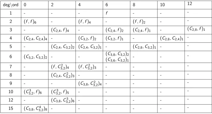
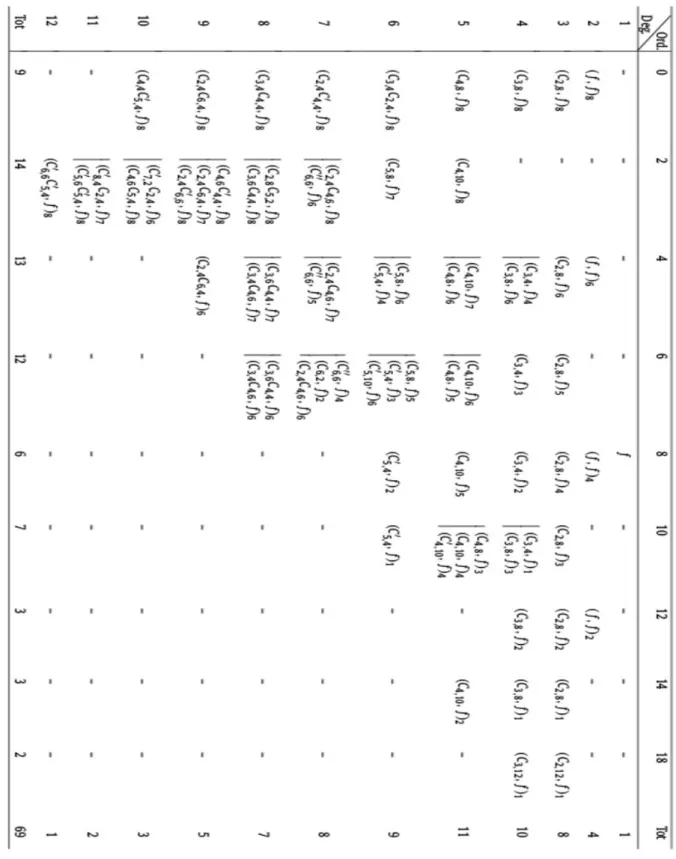
2.3.2 Base of invariants for n = 6 and n = 8. . . 34
2.3.3 Finding an isomorphism between two forms . . . 38
A binary form.sage 42
B Transvectant tables 65
C base generator 6.sage 67
D base generator 8.sage 68
Introduction
The topic of this thesis is invariant theory for binary forms. Invariant theory is a field introduced in the XIX century, first studied roughly by Cayley (1845) and later developed by Clebsch, Gordan and Hilbert (just to mention a few). The invariant theory has some theoretical applications, as well as some practical applications such as studying the properties of some algebraic objects, the simplest case being hyperelliptic curves, which corresponds to the study of binary forms (what we will be studying in this thesis). In its origins, the theory of invariants was studied more computationally. The work made by Cayley, Clebsch or Gordan used a more constructive approach, more focused in the computational and practical aspects of the theory. The great contribution of Hilbert to the field was to give a non-constructive proof of the finiteness of the algebra of invariants of binary forms, which was generalizable to forms in any number of variables (Hilbert’s basis theorem). This result had been proven by Gordan previously, but in a constructive way, and his proof was not generalizable to forms in more than two variables. The explicit computations used in the classical approach were quickly replaced by other methods, as the use of invariants required the manipulation of quite complicated polynomial expressions. In recent years, though, these explicit methods have regained interest, as the development of computers and mathematical software has given us a tool with which we can handle to some extent this complicated expressions.
The objective of this thesis is twofold. First, we want to give to the reader an introduction to invariant theory, focused on the study of binary forms. The theory explained here will be the invariant theory seen from its classical point of view, following up to certain point the exposition given by Hilbert in [2]. After this we want to give some notions to the reader about the practical applications of this theory. This we will do by exposing some of the complex problems of invariants that are only approachable computationally.
The modern approach to invariant theory studies actions of a group G on a finite vector space V,
where the invariants are functions in the space of polynomialsI ∈k[V] which are immutable by the action of G on V. The classical approach is particular case of this, which studies an action of GL2 (or SL2) on
the space of homogeneous polynomials of given number of variables and total order. This is the approach used in the exposition by Hilbert in [2] and what we will use in our thesis.
We have divided the contents of our thesis in two chapters, which separate the different objectives of our exposition:
1. Classical invariant theory: In the first chapter of the thesis we explain all the concepts and results for a basic understanding of the theory of invariants applied to binary forms.
2. Implementation: In the second chapter, we explore the more practical aspects of the theory. Here, we list some of the computational problems that we can encounter studying invariant theory and its applications. For some of these problems we have implemented a solution using a mathematical software (the program “Sage”). We describe these problems in more detail, and about the details of our implementation (the pros and cons of our solution, as well as the other possible approaches that were considered).
1. Classical invariant theory
In this first section we want to give an introduction to classical invariant theory, following mostly the ex-position from Hilbert in [2], focusing on the theory of invariants for binary forms. The objective is that the reader understands clearly the concepts of the theory of invariants (binary forms, invariants, covariants, a basis of invariants...) and the important results of the theory (characterization of invariants and covariants, the finiteness of the algebra of invariants...).
We will first introduce the basic concepts of invariant theory: forms, binary forms, invariants and covariants of forms of order n, invariants and covariants of a system of several simultaneous forms, etc... We will see that the system of invariants of binary forms of a certain order has the structure of a graded algebra and then see one of the most important results of invariant theory, that this algebra is finitely generated (Hilbert’s theorem).
After the introduction of all these basic concepts, we will see the part of the theory more oriented to the practical applications. We will introduce two methods to construct invariants and covariants that will be useful when we face the computational part of the thesis: the use of the transvectants and seeing the invariants as functions of the roots of the forms. Later we see the information the invariants give us about the form, and how to use them to know if two forms are isomorphic to each other.
1.1 Forms and binary forms
Definition 1.1. We will call a formto an homogeneous polynomial (in n variables), or what is the same, a polynomial in which every term has the same degree.
We will call a form in two variables a binary form. The same way we will call a form in three variables a ternary form, in four variables a quaternary form, etc...
For all of our work we will be studying the particular case of binary forms, so in case we do not explicitly specify the number of variables of the form, we will always be referring to forms in two variables. It is easy to see that a great part of the concepts and of the results we will be dealing with in the following sections are easily extended to forms in an arbitrary number of variables.
An arbitrary binary form of ordern can be written in the following way:
f(x1,x2) =a0x1n+ n 1 a1x1n−1x2+ ... + n i aix1n−ix2i + ... +anx2n (1)
Which is the expression we will have in mind when talking about binary forms from now on. Also, when talking about the coefficients of a form, we will be talking about the {ai} in this expression (leaving out
the binomial coefficients multiplying each term). Depending on the bibliography we are using we can see the binomial coefficients missing in the definition of a binary form. We will leave them since this is the way Hilbert presents it in [2] and most of the classical literature. The results for both ways of representing binary forms are the same, but this representation has the advantage that most of the expressions will end up being much simpler.
We will sometimes use special nomenclature to refer to binary forms of certain orders. For example, we will call binary forms of orders 2, 3, 4, 5, 6... binary quadratics, cubics, quartics, quintics, sextics, etc...
Before we continue we would want to make the following remark. For our work we will be working with the forms defined over an algebraically closed field with characteristic 0 (such asC), but it is possible
to work with binary forms and in general all of the theory defined on any field. This, though, could be a bit troublesome as some of the results we will explore along the thesis won’t work over a field not so well behaved asC. For example, we could not use the representation of binary forms just mentioned if we are
working over a field of characteristic different from 0 (because some binomial coefficients might be zero). In the classical theory of invariants binary forms were always defined overC, as Hilbert does in [2] (even if
he does not says that explicitly), so that is what we will suppose for our work. So from now on, the field of definitionk will be, unless said otherwise, an algebraically closed field of characteristic 0.
We can apply a linear transformation to the variables of a binary form in the following way:
x1=α11x10 +α12x20
x2=α21x10 +α22x20
(2)
From which we obtain a new form in the new variables x10,x20 and with coefficients ai0.
f0(x10,x20) =a00x10n+ ... + n i ai0x10n−ix20i+ ... +a0nx20n
We will always want the transformations we apply to binary forms to be invertible, that is to say that
M = α11α12
α21α22
∈GL2(k). We will also denote the transformed form asf0=f|M.
This clearly defines an action of the group GL2(k) on the set of binary forms. In some bibliography,
one can find the use of the groupSL2(k) instead ofGL2(k) for the study of invariants. The use ofSL2(k)
make some of the results for invariant theory a bit easier. This is because, as we will see later, several definitions and results in our thesis have the determinant of the transformation matrices as a factor, such as the definition of invariants 1.2and covariants 1.3. In the case we were working with SL2(k) this factor
would be just 1 and these expressions would be simpler. As we are working inCthe results for bothSL2(k)
andGL2(k) are practically the same (except for this factor of the determinant), so we will work inGL2(k)
for more generality and because this is what was used by Hilbert in [2].
Let f and g be binary forms of order n. We will call any matrix M ∈ GL2(k) such that g = f|M an
isomorphism betweenf andg. Two forms f andg will be called isomorphic if there exists an isomorphism between them.
Let f be a binary form of order n. We will call any matrix M ∈ GL2(k) such that f = f|M an
automorphism of f. The set of automorphisms of a formf is a subgroup of GL2(k).
1.2 Invariants and covariants of a form
On the center of invariant theory (as its name suggests) lie the concepts of invariant and covariant.
Definition 1.2. Let I ∈ k[a0,a1, ...,an] be a polynomial function in the coefficients of forms of order n.
We will say that I is an invariant if for any linear transformation M, I changes by a fixed power of the determinant ofM, or what is the same:
I(a00,a01, ...,a0n) =det(M)pI(a0,a1, ...,an) (3)
Definition 1.3. Let C ∈k[a0,a1, ...,an;x1,x2] be a polynomial function in both the coefficients of forms
of order n and the two variables x1 and x2. We will say that the expression C is a covariant if for any
linear transformationM,C changes by a fixed power of the determinant ofM, or what is the same:
C(a00,a01, ...,an0,x10,x20) =det(M)pC(a0,a1, ...,an,x1,x2) (4)
wherea0i andx10,x20 are the new coefficients and variables after the application ofM.
To avoid misunderstandings about nomenclature in the work, we will explain briefly the few basic terms that we will be using when talking about forms, invariants and covariants that can be confused (especially
between the termsorder and degree):
1. LetI =P
Zaν0
0 a
ν1
1 ...aνnn be an invariant for forms of ordern, and lett=Za0ν0a
ν1
1 ...aνnn be a summand
of the invariant. We will call to the expression:
g =ν0+ν1+ ... +νn
the “degree” of t. Also, as we will see later, an invariant must be an homogeneous polynomial in the{ai}, what means that all its terms must have the same degree g. We will call the “degree” of
I to the degree that share all of its terms.
2. LetI =P
Zaν0
0 a
ν1
1 ...aνnn be an invariant for forms of ordern, and lett=Za
ν0
0 a
ν1
1 ...aνnn be a summand
of the invariant. We will call to the expression:
p =ν1+ 2ν2+ ...nνn
the “weight” of t. In the same way as with the degree, we will see later that an invariant must be an isobaric polynomial in the{ai}. This means that all its terms must have the same weight p. We
will call the “weight” of I to the weight that share all of its terms.
3. LetC be a covariant for forms of ordern. As we will see later, a covariant must be an homogeneous polynomial in the xi. We will call the order of C as a polynomial in thex the “order” of C and we
will usually denote it with anm.
Note from the definitions of invariant and covariant that the first is a particular case of the second. So one could say that an invariant is just a covariant of order 0.
We can list some examples of invariants and covariants of simple binary forms:
Example 1.4. For the binary quadratic form f(x1,x2) = a0x12 + 2a1x1x2 +a2x22 we can only make one
invariant of degree 2 (except scalar multiples of it), which is known as the discriminant of the form:
I =a0a2−a21
Example 1.5. For the binary quarticf(x1,x2) =a0x14+ 4a1x13x2+ 6a2x12x22+ 4a3x1x23+a4x24 we can only
make one invariant of degree 2 (except scalar multiples of it), which is:
I =a0a4−4a1a3+ 3a22
Example 1.6. For any order n, the expression for a binary form is in itself a covariant C = f =
a0x1n+
n
1
a1x1n−1x2+ ... +anx2n. Easily we can see that C satisfies the covariant property: for any linear
transformation M ∈GL2(k), by applying it to C the covariant remains the same in the new coefficients
We have not shown that these examples really satisfy the invariant property. We could check this directly by the definition of invariant, by applying a generalized linear transformation to the original form and checking that the transformed polynomial is the same (up to a power of the determinant of the trans-formation matrix). Instead of that, we will introduce the following concepts that will help us characterize when an expression is an invariant/covariant.
Definition 1.7. LetI =P
Zv0v1...vna
v0
0 ...avnn be a polynomial expression in the coefficients of forms of order
n, we define the operatorsDand ∆ as follows
D=a0 ∂ ∂a1 + 2a1 ∂ ∂a2 + ... +nan−1 ∂ ∂an ∆ =na1 ∂ ∂a0 + (n−1)a2 ∂ ∂a1 + ... +an ∂ ∂an−1 (5)
These concepts can be used to find sufficient conditions for an expression to be an invariant by linear transformations. These are given in the following theorem:
Theorem 1.8. Let I(a0, ...,an) be a polynomial expression in the coefficients of forms of order n. The
expression I is an invariant by linear transformations in GL2(k) with exponent p if and only if it satisfies
the following properties:
1. It is an homogeneous polynomial of degree g , isobaric of weight p, and its degree and weight satisfy the relation ng = 2p.
2. It satisfies the equation DI = 0. 3. It satisfies the equation ∆I = 0.
Proof. Every linear transformation M = α11α12
α21α22
∈GL2(K) can be expressed as a product of the three
following types of linear transformations:
1. κ 0 0 λ 2. 1 ν 0 1 3. 1 0 µ 1
the proof of this fact is a basic linear algebra exercise.
It follows from this statement that an expression in the coefficients of a binary form that satisfies the invariant property for any linear transformation of the types1,2 and3 would be an invariant of the binary form. What we will do to prove the theorem is to see for each of these three types of linear transformations how they affect the coefficients {ai} of the form, and what properties needs to have an expression to be
invariant by each kind of transformation. The conditions we give in the theorem for an expression to be an invariant will be a consequence from these facts.
1. The application of transformation 1 to the binary formf =a0x1n+ n 1 a1x1n−1x2+ ... +anx2n results in: f0=f(κx10,λx20) =a0κnx10n+ n i a1κn−1λx10n−1x 0 2+ ... +anλnx20n =a00x10n+ n i a10x10n−1x20 + ... +a0nx20n
So if we compare the two expressions we end up with then+ 1 relations:
a0i =κn−iλiai
Now we study what happens to a polynomial expression on the {ai} when evaluated in the new
coefficients. If we have one such expression, namelyI({ai}) =PZaν00a
ν1 1 ...aνnn, then we have: I({a0i}) =XZa0ν0 0 a 0ν1 1 ...a 0νn n =XZaν0 0 a ν1 1 ...a νn n κnν0+(n −1)ν1+...+νn−1λν1+2ν2+...+nνn
Now, for this expression to be an invariant respect to this kind of transformation, we would need that, according to the definition of invariant, for a certain numberp:
I({a0i}) =det(M)pI({ai}) =κpλpI({ai})
For this to work every term of the sum must fulfill the equality. Then, comparing the two expressions, we obtain the identities:
nν0+ (n−1)ν1+ ... + (n−i)νi + ... +νn−1=p
ν1+ 2ν2+ ... +iνi+ ... +nνn=p
Now we see that this is precisely the definition of weight we gave earlier. Also, if we add together the two equations, we obtain:
n(ν0+ν1+ ... +νn) =ng = 2p
So with this we have seen that, for a polynomial expressionI({ai}) to be invariant by a transformation
of type1, beingpthe exponent of the transformation determinant by which the invariant is multiplied upon transformation, it has to be an isobaric function of weight equal to p, homogeneous of degree
g satisfying both the equation ng = 2p. This gives us the first point of the theorem.
2. Similarly to the previous one, we want to see what happens to the binary form f = a0x1n +
n
1
a1x1n−1x2+ ... +anx2n after applying a general linear transformation of the type2:
f0 =f(x10 +νx20,x20) =a0(x10 +νx 0 2)n+ n 1 a1(x10 +νx 0 2)n −1x0 2+ ... +anx20n =a00x10n+ n 1 a01x10n−1x2+ ... +an0x 0n 2
We want to obtain, as in the previous case, a relation between the{a0i} and the{ai}. If we compare
the coefficients of the termsx1ix2n−i, we obtain:
n i a0i = n i ai + n i−1 (n−i+ 1)ai−1ν+ ... + n i−k n−i +k k ai−kνk + ... +a0νi
and because of the identity:
n i−k n−i+k k = n i i k
we have the following relation between the transformed coefficients{a0i} and the old ones{ai}:
ai0 =ai + i 1 ai−1ν+ ... + i k ai−kνk+ ... +a0νi
Now, for a polynomial expression on the coefficients I({ai}) to be invariant by transformations of
this type, one has to have:
I({a0i}) =det(M)pI({ai}) =I({ai})
We want to find which properties has to have this expression to remain invariant for any transformation of type 2, so this equation should hold by any possible value of ν. With this being true, we can derive in both sides respect toν, obtaining:
∂I({ai0}) ∂a00 ∂a00 ∂ν + ∂I({ai0}) ∂a01 ∂a01 ∂ν + ... + ∂I({a0i}) ∂a0 n ∂a0n ∂ν = 0
But if we look at the development of ∂a
0 i ∂ν we see that: ∂a00 ∂ν = 0 ∂a10 ∂ν =a0 =a 0 0 ∂a20 ∂ν = 2a1+ 2a0ν = 2a 0 1 ... ∂a0i ∂ν =iai−1+ ... + i k kai−kνk−1+ ... +ia0νi−1 =iai−1+ ... + i−1 k−1 iai−kνk−1+ ... +ia0νi−1 =ia0i−1
which transforms the previous equation in:
∂I({a0i}) ∂a00 ∗0 + ∂I({a0i}) ∂a01 a 0 0+ ... + ∂I({ai0}) ∂a0 n na0n−1= 0
But this is the operator D we defined earlier. So, in the end, this gives us the second point in our theorem:
For a polynomial expression I({ai}) in the coefficients of a form to be invariant by linear
transfor-mations of the type2, the expressionI must satisfy the equation:
3. The analysis for the third kind of transformations is very similar to the one done for the second type. We will proceed in the same fashion:
For a binary form f =a0x1n+ n1
a1x1n−1x2+ ... +anx2n, if we apply to it a linear transformation of
the type 3, we obtain:
f0 =f(x10,µx10 +x20) =a0x10n+ n 1 a1x10n−1(µx 0 1+x 0 2) + ... +an(µx10 +x 0 2)n =a00x10n+ n 1 a10x10n−1x20 + ... +a0nx20n
With arguments similar to the ones applied to the transformations of type2 one has the relations:
ai0 =ai + n−i 1 ai+1µ+ ... + n−i k ai+kµk + ... +anµn−i
And for later, if we derive these terms byµ, one has the equivalences:
∂a0i ∂µ = (n−i)ai+1+ ... + n−i k kai+kµk−1+ ... + (n−i)anµn−i−1 = (n−i)ai+1+ ... + n−i−1 k−1 (n−i)ai+kµk−1+ ... + (n−i)anµn−i−1 = (n−i)a0i+1
For a polynomial expressionI({ai}) to be invariant respect to transformations of the type3one must
have:
I({a0i}) =det(M)pI({ai}) =I({ai})
and if we derive both sides byµwe obtain the equation:
∂I({a0i}) ∂a00 na 0 1+ ... + ∂I({ai0}) ∂a0i (n−i)a 0 i+1+ ... + ∂I({a0i}) ∂a0 n ∗0 = 0
Which we see again that is equal to the operator ∆ we defined before. So with this we have the third condition for our theorem:
A polynomial expression I({ai}) in the coefficients of a binary form is invariant by transformations
of the type3 if it satisfies the equation:
∆I = 0
With this we have seen that in order for an expressionI({ai}) to be invariant by linear transformations
of the types1,2and3it has to satisfy all the conditions listed in the theorem. Because any transformation
M ∈GL2(K) can be written as a product of transformations of these three types, any expression I that
satisfies the conditions listed will be an invariant.
The concepts introduced before are the same applied to polynomials in k[{ai},x0,x1], so we can also
apply them to determine the sufficient conditions for covariants of binary forms. But before we give these conditions for covariants we want to make a quick remark. We will suppose from now on, and without loss of generality, that covariants are polynomials homogeneous in the variables xi. We do this because of the
each homogeneous function of the xi transforms into an homogeneous function of the same order. This
implies that if a polynomial function ink[{ai},x0,x1] (not necessarily homogeneous) satisfies the covariant
property, then each of its homogeneous parts are also covariants. So we can consider only the homogeneous covariants for our study.
With this in mind, let us see the set of conditions for an expression to be a covariant:
Theorem 1.9. Let C(a0, ...,an,x1,x2) be a polynomial expression in the coefficients of forms of order n
and the variables x1,x2, and that is homogeneous in the xi. The expression C is a covariant by linear
transformations in GL2(k) with exponent p if and only if it satisfies the following properties:
1. Written as C = C0x1m + ... +Cix1m−ix2i + ... +Cmx2m each Ci is an homogeneous polynomial in
the coefficients ai of the same degree g and isobaric of weight p+i , and C satisfies the equation
m=ng−2p
2. It satisfies the equation DC =x2∂∂x1C
3. It satisfies the equation ∆C =x1∂∂x2C
Proof. The proof for this theorem will follow the same steps as the previous one. We will see for each of the three types of linear transformations that we mentioned above, which properties make an expression to be a covariant respect to transformation of that type, and we will see that joining the three parts together we obtain our theorem.
1. We know from the last theorem’s proof the way a binary form is modified by transformations of type 1 and the relation existing between the new coefficients {a0i} after the transformation and the
original ones {ai}. Now we want to know how does this affect to a polynomial expression like
C(a0,a1, ...,an,x1,x2), to find the conditions for it to be a covariant respect to this transformation.
As we said earlier, we can consider the polynomial homogeneous in the variables xi, so, let us call m
the order of C in the variablesxi, and let us represent this polynomial as:
C =C0x1m+C1x1m−1x2+ ... +Cmx2m
where each of the Ci is (as we denoted in the previous proof) Ci =PZaν00a
ν1
1 ...anνn. Now, for this
expression to be a covariant, it must satisfy the covariant property for this kind of transformations,
namely, for some number p:
C({a0i},x10,x20) =det(M)pC({ai},x1,x2) =κpλpC({ai},x1,x2)
If we work out the expression for C({a0i},x10,x20) with the relations between the {a0i} and the {ai}
worked out in the previous proof, we obtain:
C({a0i},x10,x20) =C({aiκn−iλi}, x1 κ, x2 λ) =C0({a 0 i}) x1m κm +C1({a 0 i}) x1m−1 κm−1 x2 λ + ... +Cm({a 0 i}) x2m λm
And if we now compare the coefficients ofx1m−ix2i in both sides of the equation, we find out:
Ci(a00, ...,an0)κi−mλ−i = X Zaν0 0 a ν1 1 ...anνnκnν0+(n−1)ν1+...+νn−1λν1+2ν2+...+nνnκi−mλ−i =κpλpXZaν0 0 a ν1 1 ...aνnn
with the same argument as in the last proof, we obtain from this the following two equations:
nν0+ (n−1)ν1+ ... +νn−1+i−m=p
ν1+ 2ν2+ ... +nνn−i =p
and adding the two together we obtain the following relation:
n(ν0+ν1+ ... +νn)−m=ng−m= 2p
As every term on the sum must satisfy these equations, we can extract the following information from this:
For the expression C to be a covariant by the transformations of type 1, as these equations must hold for all terms, each of the terms Ci must be isobaric of weight equal to p+i and homogeneous
of degreeg, which satisfies the equation ng−m= 2p
2. For the study of transformation of type 2 we proceed also in the same way as before. Because for
transformationsMof type2one has thatdet(M) = 1, then for a polynomial expressionC({ai},x1,x2)
to be a covariant respect to it, it must satisfy:
C({a0i},x10,x20) =C({ai},x1,x2) (6)
All the relations computed in the previous proof are the same here, so we can use them in the same way: a0i =ai + i 1 ai−1ν+ ... + i k ai−kνk+ ... +a0νi x10 =x1−νx2 x20 =x2
We want to proceed in the same way as before, so we want to derivate both sides of the equation 6
with respect toν, so we have:
∂C({a0i}) ∂a00 ∂a00 ν + ... + ∂C({a0i}) ∂a0n ∂a0n ν + ∂C({a0i}) ∂x10 ∂x10 ν + ∂C({ai0}) ∂x20 ∂x20 ν = ∂C({a 0 i}) ∂a00 ∗0 + ∂C({a0i}) ∂a10 a 0 0+ ... + ∂C({a0i}) ∂a0 n nan0−1−∂C({a 0 i}) ∂x10 ∗x 0 2+ ∂C({a0i}) ∂x20 ∗0 = 0
As we see, this again contains the application of the operatorD. For the same reasons as before, this equation must hold for all values of ν, so we can obtain from here the condition for an expression to be covariant by transformations of type2:
A polynomial expression C({ai0},x10,x20) is covariant by transformations of type 2 if and only if it satisfies the equation:
DC −x2
∂C
∂x1
= 0 which gives us the second condition in the theorem.
3. The same is done for transformations of type3. Because transformationsMof type3havedet(M) = 1, for any polynomial expression C({ai},x1,x2) to be covariant respect to transformations of this
type, it must satisfy again the equation6.
We can retrieve the relations between the primed variables and the original ones from the previous proof: a0i =ai + n−i 1 ai+1µ+ ... + n−i k ai+kµk + ... +anµn−i x10 =x1 x20 =−µx1+x2
And from this we may proceed in the same fashion. We want to derive both sides of equation6 by
µ, as this equation must hold for every possible value ofµ. Doing this we obtain:
∂C({a0i}) ∂a00 ∂a00 µ + ... + ∂C({a0i}) ∂a0n ∂a0n µ + ∂C({a0i}) ∂x10 ∂x10 µ + ∂C({a0i}) ∂x20 ∂x20 µ = ∂C({a 0 i}) ∂a00 na 0 1+ ∂C({a0i}) ∂a01 (n−1)a 0 2+ ... + ∂C({a0i}) ∂a0n ∗0 + ∂C({a0i}) ∂x10 ∗0− ∂C({a0i}) ∂x20 ∗x 0 1 = 0
Again we can see in the development of the equation the operator ∆. From this we obtain the third condition of the statement:
For a polynomial expression C({ai},x1,x2) to be a covariant by transformations of type3, it must
satisfy the equation:
∆C −x1
∂C
∂x2
= 0
This is the easy characterization of invariants and covariants, but this set of conditions can still be reduced. Next we present the minimum set of conditions for a polynomial expression to be an invariant/-covariant of a given form:
Theorem 1.10. A polynomial expression I in the coefficients{ai}is an invariant for binary forms of order
n if and only if:
1. It is an homogeneous and isobaric polynomial and its degree and weight satisfy the equation ng = 2p 2. It satisfies the equation D I = 0
Theorem 1.11. A polynomial expression C in the coefficients {ai} and variables x1,x2 which is
homoge-neous in the xi is a covariant for binary forms of order n if and only if:
1. Written as: C =C0x1m+C1x1m−1x2 + ... +Cmx2m, the term C0 is a homogeneous polynomial of
degree g and isobaric of weight p and satisfy the equation m=ng−2p 2. The term C0 satisfy the equationDC0 = 0
3. Each of the other terms Ci satisfies the condition:
Ci =
(m−i)!
m! ∆
iC
The term C0 is called the source of the covariant. As we see from the last theorem, it is important
because one can determine the whole covariant from it.
The proof of these two theorems can be found in [2, chap. I.6]. We omit the proof because in order to make it we would need to explain in detail some non-trivial properties of the two operators D and ∆. These properties can take a bit long to prove, and since they are only interesting to us as a mean to prove these theorems, we will leave them out.
1.3 Simultaneous invariants and covariants
We have defined an invariant as a polynomial in the coefficients of binary forms that satisfies the invariant property (that it is invariant by lineal transformations). We can generalize this concept to apply it to a system of more than one form, producing the concept of simultaneous invariants.
If we consider a system of more than one form at a time:
f =a0x1n1+ n1 1 a1x1n1−1x2+ ... +an1x2n1 g =b0x1n2+ n2 1 b1x1n2−1x2+ ... +bn2x2n2 ...
we can apply a linear transformation to the whole system, obtaining:
f|M =a00x10n1+ n1 1 a10x10n1−1x20 + ... +a0n1x20n1 g|M =b00x 0n2 1 + n2 1 b10x10n2−1x20 + ... +bn20 x20n2 ...
With this, we can define the same concepts of invariants and covariants for a system of several forms at once. We give the definition for a system of two simultaneous forms, since the generalization from here is obvious:
Definition 1.12. Let I({ai},{bi}) be a polynomial expression in the coefficients of a system of two forms
of ordersn1 andn2. The expressionI is said to be an invariant if it satisfies the invariant property, namely:
For any linear transformation M ∈GL2(k), the expression in the new coefficients ({ai0},{bi0}) remains
the same (up to a fixed power of the determinant of the transformation matrix):
I({a0i},{b0i}) =det(M)pI({ai},{bi})
One can see that this concept is easily generalized from two binary forms to any number of forms, being then the invariantI an expression in the coefficients of all the binary forms involved.
The same way as with invariants, we can also generalize the concept of covariant to simultaneous covariants of any number of forms (in the same way we did with invariants).
Definition 1.13. LetC({ai},{bi},x1,x2) be a polynomial expression in the coefficients of a system of two
binary forms of orders n1 andn2, as well as in the two variablesx1,x2. Then, the expressionC is said to
For any linear transformation M ∈GL2(k), the expression in the new coefficients ({ai0},{bi0}) remains
the same (up to a fixed power of the determinant of the transformation matrix):
C({a0i},{bi0},x10,x20) =det(M)pI({ai},{bi},x1,x2)
This time again, is immediate to generalize this concept from two binary forms to any number of forms. Now we may want from the invariants/covariants of two or more forms the same kind of characterization as we had for invariants/covariants of a single form (giving us a simple way to check if an expression was an invariant/covariant). We will explain the conditions for invariants/covariants of two forms and (again) it will be clear how to extend this characterization to any number of forms.
Definition 1.14. Given two binary formsf1,f2 with orders n,mand coefficients{ai},{bi} respectively, for
a monomialM =Zav00 av11 ...avn
nbw00 ...bmwm on the coefficients of the forms, we define its weight as:
p =v1+ 2v2+ ... +nvn+w1+ ... +mwm (8)
Definition 1.15. Given two binary formsf1,f2 with orders n,mand coefficients {ai},{bi}respectively, we
define the following operators:
Da =a0 ∂ ∂a1 + 2a1 ∂ ∂a2 + ... +nan−1 ∂ ∂an Db =b0 ∂ ∂b1 + 2b1 ∂ ∂b2 + ... +mbm−1 ∂ ∂bm ∆a=na1 ∂ ∂a0 + (n−1)a2 ∂ ∂a1 + ... +an ∂ ∂an−1 ∆b=mb1 ∂ ∂b0 + (m−1)b2 ∂ ∂b1 + ... +bm ∂ ∂bm−1 D=Da+Db ∆ = ∆a+ ∆b
With these definitions we can now specify the conditions for an expression to be a simultaneous invari-ant/covariant of a set of binary forms (as in the rest of the section, we state the theorem for simultaneous invariants/covariants of two forms, as the extension to any number of forms is direct).
Theorem 1.16. Let I({ai},{bi})be a polynomial function in the coefficients of forms of orders n1 and n2
respectively. Then, the expression I is a simultaneous invariant if and only if:
1. it is an isobaric polynomial of weight p, as a polynomial of the{ai}is homogeneous of degree g1, as
a polynomial of the{bi}is homogeneous of degree g2 and it satisfies the equation n1g1+n2g2= 2p
2. it satisfies the equationDI = 0
Theorem 1.17. Let C({ai},{bi},x1,x2) be a polynomial function in the coefficients of forms of orders n1
and n2 and the variables x1,x2, which is homogeneous as a polynomial in the xi. Then, C is a simultaneous
1. Written as C =C0x1m+...+Cmx2m, the term C0is an isobaric polynomial of weight p, as a polynomial
in the ai is homogeneous of degree g1 and as a polynomial in the bi is homogeneous of degree g2,
and it satisfies the equation m=n1g1+n2g2−2p
2. The term C0 satisfiesDC0 = 0
3. Each of the rest Ci satisfy the equation:
Ci =
(m−i)!
m! ∆
iC
0
The complete proof of these two theorems can be found in [2, chap. I.9]. They follow the same steps as the proofs for the characterization of invariants/covariants of just one binary form, just generalizing each step for considering we are working with two binary forms, but the process is the same. We won’t include them since they do not contribute anything new to the thesis.
1.4 Basis of invariants
The set of invariants of binary forms of ordernwill be an essential part of our work. So we want to know a bit more about its structure. Let us look at some of the properties that have the set of invariants of forms of order n:
1. Let I be an invariant of forms of ordern that has degree g and weightp. An scalar multiple of the invariantλI is also an invariant for forms of ordern with degreeg and weightp.
2. Let I1 and I2 be two invariant of forms of order n that have degrees g1,g2 and weights p1,p2
respectively. The product I1I2 of the two invariants is also an invariant for forms of order n which
has degreeg1+g2 and weightp1+p2.
This is clear looking at it from the pure definition of invariant. Letf1 andf2 be binary forms of order
n andM ∈GL2(k) such thatf2 =f1|M. Then:
I1(f2) =det(M)p1I1(f1)
I2(f2) =det(M)p2I2(f1)
and so:
(I1I2)(f2) =det(M)p1+p2(I1I2)(f1)
3. Let I1 andI2 be two invariants of forms of order n with the same degree g and weightp. Then the
sum of the two invariants, namelyI1+I2, is also an invariant of forms of ordern with degreeg and
weight p.
This is again clear just by looking at the definition:
(I1+I2)(f2) =det(M)pI1(f1) +det(M)pI2(f1) =det(M)p(I1+I2)(f1)
With these properties we can state the following:
We will make a brief remark about this statement. When we talk about invariants we want to move in this “algebra of invariants”, but because the sum of two invariants of different degree is not really an invariant, the elements of the algebra might not be necessarily invariants. Instead, the elements of the algebra of invariants are sums of invariants of different degree, for which each homogeneous part is an invariant.
This result (that the invariants have structure of an algebra) is not only true for binary forms, but also for forms in any number of variables (ternary forms, quaternary forms etc...) and even for systems of simultaneous forms.
One of the most important questions that surged in invariant theory when it was first studied (Cayley) was if the algebra of invariants for a system of simultaneous forms is or not finitely generated. This is indeed true, and we can state it as follows:
Theorem 1.19. Hilbert’s theorem. The algebra of invariants for binary forms of order n is finitely generated, for any arbitrary value of n.
This is one of the most important results of invariant theory. When Cayley began studying invariant theory, he made this conjecture but could not prove it more than for the particular cases of binary forms up to order 6. Later, Gordan proved this result for a system of an arbitrary number of binary forms, but could not prove it for forms in more than two variables. It was Hilbert who found a generalizable proof of this theorem for forms in any number of variables.
In [2, chap. II] one can find two proofs of this theorem from Hilbert. The first one is a proof of the theorem using the representation of invariants as function of the roots of the forms. The second, more complex, is a generalizable proof for forms of any number of variables. We do not include any of these proofs in our work because of their extension and complexity.
Because of this result we know that, for binary forms of ordern, there exists a finite number of invariants that generate the algebra of invariants for these forms. We will call this finite set of invariants abasis for the algebra of invariants of order n. This is an important concept that we will use a lot in the thesis. We could list some examples:
Example 1.20. For binary forms of order 2, every invariant can be written as a polynomial function of one invariant of degree 2 (the discriminant I =a0a2−a12). This only invariant is the basis for the algebra of
invariants of order 2.
Example 1.21. For binary forms of order 4, every invariant can be written as a polynomial function of two invariants of degrees 2 and 3:
I2 =a0a4−4a1a3+ 3a22
I3 =a0a2a4−a0a23−a21a4+ 2a1a2a3−a32
so these two invariants are a basis for the algebra of invariants of order 4. We will prove this particular result in the next section.
For the algebra of invariants of a given order, the basis of invariants is not unique. In fact, for some cases there are different interesting bases that have been used in the literature. As, for example, for the algebra of invariants of order 6, we can encounter in the literature the bases of Igusa (I2,I4,I6,I10,I15),
Clebsch (C2,C4,C6,C10,R), etc... which are named after the person who introduced them. We will be
1.5 Number of invariants
Now that we have the characterization of invariants and covariants, the question arises of how many invariants can be found for a given form of a certain degree and weight.
First of all it must be noticed from the properties shown in the previous section that any linear com-bination of two invariants of the same weight is yet another invariant for the same base form. Thus, the invariants of degreeg and weightp generate a vector space, and there are an infinite number of invariants for a given form. What we will be interested in, though, is the dimension of this space, or what is the same, the number of linearly independent invariants of degree g and weightp.
Let us callMn(g,p) the set of monomials of the ringZ[{ai}] with coefficient 1 that have degreeg and
weight p, and let us callmn(g,p) the cardinal of this set.
Theorem 1.22. The number of linearly independent invariants of degree g and weight p for forms of order n, which we will call wn(g,p) is given by the formula:
wn(g,p) =mn(g,p)−mn(g,p−1) (9)
We can give an intuitive notion of why this holds. The invariants for forms of ordern can be expressed
as I =P
Zaν0
0 a
ν1
1 ...aνnn, and if we want them to be of degree g and weightp the exponents must satisfy:
ν0+ν1+ ... +νn=g
ν1+ 2ν2+ ... +nνn=p
there are mn(g,p) possible values for the exponents, so the sum can have this number of summands.
Now, forI to be an invariant it must satisfy the equationDI =P
ZDaν0
0 a
ν1
1 ...aνnn = 0. As the operator D
applied to a term of degreeg and weightp results in an homogeneous polynomial of degreeg and isobaric of weight p−1, we havemn(g,p−1) distinct summands in the expression of DI. As every term of this
sum must banish, we end up with mn(g,p−1) linear equations for the coefficients Z that must be equal
to 0.
Now, we have mn(g,p −1) linear equations for the mn(g,p) coefficients Z of the sum. We could
choose arbitrarilymn(g,p)−mn(g,p−1) coefficients, assign them a value, and the rest would be uniquely
determined. We can assign values for the mn(g,p)−mn(g,p−1) coefficients Z chosen in as much as
mn(g,p)−mn(g,p−1) linearly independent ways. This gives the number of invariants one can generate
of degreeg and weightp.
This is not a proof of the theorem. Note that we have not argued that the system of mn(g,p−1)
equations are linearly independent. We won’t include the complete proof here, as it is a bit larger than this and needs use of some results that we have not introduced. But the full proof of the theorem can be found in [2, p. 50].
Now we want expressions for the quantitiesmn(g,p) andwn(g,p).
Because the weight of an invariant is determined given the order and degree by the equation ng = 2p, one can write the previous formula as:
wn(g) =wn(g, ng 2 ) =mn(g, ng 2 )−mn(g, ng 2 −1) (10)
Using combinatorial arguments one can find expressions for the numbers mn(g,p) and thus, also for
Theorem 1.23. The cardinal of the set Mn(g,p) is given by the formula: mn(g,p) = (1−xn+1)(1−xn+2)...(1−xn+g) (1−x)(1−x2)...(1−xg) xp (11)
where[f]xk denotes the coefficient of degree k of the Taylor series of the function f . Proof. First we will see thatmn(g,p) admits the following representation:
mn(g,p) = 1 (1−y)(1−xy)(1−x2y)...(1−xny) xpyg (12) This will follow from the combinatorial interpretation ofmn(g,p). If we break the expression we get:
1
(1−y)(1−xy)(1−x2y)...(1−xny) =
(1 +y+y2+ ...)(1 +xy+x2y2+ ...)(1 +x2y+x4y2+ ...)...(1 +xny+x2ny2+ ...) and the general term of this expansion could be expressed as:
yν0(xy)ν1...(xny)νn =xν1+2ν2+...+nνnyν0+ν1+...+νn
so for the general expansion, the coefficient for the termxpyg will be the number of ways one can express
p asν1+ 2ν2+ ... +nνn andg asν0+ν1+ ... +νnsimultaneously. This is equal to the numbermn(g,p).
We have proven that the number mn(g,p) satisfy the equation 12 as the coefficient of xpyg of the
Taylor expansion of a function in x and y. We will now show how we can get from this formula to the
formula given in the statement.
We want to get rid of the variabley on our formula. We can expand the expression as a polynomial in this variable and write it as:
1
(1−y)(1−xy)(1−x2y)...(1−xny) = 1 +C1y+C2y
2+ ...
on every Ci is a polynomial in thex only. Now, because we have:
(1−y) 1
(1−y)(1−xy)(1−x2y)...(1−xny) = (1−x
n+1y) 1
(1−xy)(1−x2y)(1−x3y)...(1−xn+1y)
expanding both sides as polynomials in y
(1−y)(1 +C1y+C2y2+ ...) = (1−xn+1y)(1 +C1xy +C2x2y2+ ...)
and comparing the coefficients in both sides of the term foryg we obtain the equation:
Cg −Cg−1=xgCg −xn+gCg−1
and:
Cg =
1−xn+g
1−xg Cg−1
If we apply iteratively this relation for Cg,Cg−1...C2,C1, then we obtain that:
Cg =
(1−xn+1)(1−xn+2)...(1−xn+g) (1−x)(1−x2)...(1−xg)
And we can see the statement in the theorem is a direct consequence of this: mn(g,p) = 1 (1−y)(1−xy)(1−x2y)...(1−xny) xpyg = [Cg]xp = (1−xn+1)(1−xn+2)...(1−xn+g) (1−x)(1−x2)...(1−xg) xp
Theorem 1.24. The number of linearly independent invariants of degree g for a form of order n is given by the formula: wn(g) = (1−xn+1)(1−xn+2)...(1−xn+g) (1−x2)(1−x3)...(1−xg) xng2 (13)
Proof. With the result for mn(g,p) we can proof the result for wn(g) quite easily. If we expand the
expression formn(g,p) as a Taylor series:
mn(g,p) = (1−xn+1)(1−xn+2)...(1−xn+g) (1−x)(1−x2)...(1−xg) xp =c0+c1x+c2x2+ ... +cpxp+ ... xp =cp
So if we develop both sides of the equation in the statement separately we obtain, in one side:
wn(g) =mn(g,p)−mn(g,p−1) =cp−cp−1
where herep = ng2 . In the other side, we obtain:
(1−xn+1)(1−xn+2)...(1−xn+g) (1−x2)(1−x3)...(1−xg) xp = (1−x)(1−x n+1)(1−xn+2)...(1−xn+g) (1−x)(1−x2)(1−x3)...(1−xg) xp =(1−x)(c0+c1x+c2x2+ ... +cpxp+ ...) xp =c0+ (c1−c0)x+ (c2−c1)x2+ ... + (cp−cp−1)xp+ ... xp =cp−cp−1
So we have proven that:
wn(g) =cng 2 −c ng 2−1= (1−xn+1)(1−xn+2)...(1−xn+g) (1−x2)(1−x3)...(1−xg) xng2
With this result we can find out easily how many invariants does a binary form has of a certain degree. But this result can also be used to work out (by working with the general expression in function ofg) which invariants generate the algebra of invariants for forms of that order. Here we give an example of how to do this:
Example 1.25. For binary forms of ordern= 4 we have that p= 2g, so one has that:
w4(g) = (1−x5)(1−x6)...(1−x4+g) (1−x2)(1−x3)...(1−xg) x2g
or what is the same w4(g) = (1−xg+1)(1−xg+2)...(1−x4+g) (1−x2)(1−x3)(1−x4) x2g
If we operate this expression we obtain the following:
w4(g) = (1−xg+1)(1−xg+2)...(1−x4+g) (1−x2)(1−x3)(1−x4) x2g = 1−xg+1−xg+2−xg+3−xg+4 (1−x2)(1−x3)(1−x4) x2g = 1 (1−x2)(1−x3)(1−x4) x2g − xg+1(1 +x+x2+x3) (1−x2)(1−x3)(1−x4) x2g = 1 (1−x2)(1−x3)(1−x4) x2g − xg+1 (1−x)(1−x2)(1−x3) x2g = 1 (1−x2)(1−x3)(1−x4) x2g − x (1−x)(1−x2)(1−x3) xg = 1 (1−x2)(1−x3)(1−x4) x2g − x2 (1−x2)(1−x4)(1−x6) x2g = (1−x6)−x2(1−x3) (1−x2)(1−x3)(1−x4)(1−x6) x2g = 1−x2+x3 (1−x2)(1−x4)(1−x6) x2g = 1−x2 (1−x2)(1−x4)(1−x6) x2g + 0 = 1 (1−x4)(1−x6) x2g = 1 (1−x2)(1−x3) xg
What can be derived from this calculation is the following: The number of invariants for a binary quartic of degree g is w4(g) = 1 (1−x2)(1−x3) xg = (1 +x2+x4+x6+ ...)(1 +x3+x6+x9+ ...) xg
and we will have that there are as many invariants of orderg as there are non-negative integer solutions for k,l of the equation:
2k+ 3l =g
For g = 2 andg = 3 we have just one invariant for the binary quartic, namely:
I2 =a0a4−4a1a3+ 3a22
I3 =a0a2a4−a0a23−a21a4+ 2a1a2a3−a32
and we have that for every k,l the expression I =I2kI3l is also an invariant of degree g = 2k+ 3l. As we can do this for every k,l that add up tog, we can obtain all the invariants of degreeg in this manner.
Therefor we have that the invariants I2 and I3 are generators of the algebra of invariants for the binary
quartic, or what is the same, that all the invariants of the binary quartic can be expressed as a polynomial expression of the two invariants I2 andI3.
1.6 Transvections
Until now we have explored the properties of invariants and covariants, and found a simple way to determine if given expressions were or not invariants or covariants of binary forms. But what we do not have is a systematic way for finding the invariants and covariants of a form. Here we introduce the concept of transvectant (or transvection), which will allow us to do exactly that.
Definition 1.26. Given two binary forms f1,f2 of orders n1,n2 and coefficients {ai},{bi} we define the
transvectantof orderp (orp-th transvectant) as the simultaneous covariant of the two forms that has as its source the following expression:
C0= p X i=0 (−1)i p i aibp−i
We will denote the resulting covariant (the transvectant) as (f1,f2)p, and it is a covariant of degree
g = 2, weightp and order m=n1+n2−2p.
One can check easily that this expression generates indeed a simultaneous covariant of the two forms. If we look at the characterization of simultaneous covariants in1.17, we see that:
1. the first condition holds clearly. It is clear that the expression forC0 is homogeneous both in the{ai}
and in the{bi}and that it is an isobaric polynomial with weight equal toi+p−i =p. We can see
that (with the same notation as in1.17)g1 =g2 = 1, and thenm=n1g1+n2g2−2p =n1+n2−2p.
2. If we operate the expressionDC0, we get: DC0 =D p X i=0 (−1)i p i aibp−i = p X i=0 D(−1)i p i aibp−i = p X i=0 (−1)i p i [iai−1bp−i + (p−i)aibp−i−1] = p X i=1 (−1)i p i iai−1bp−i+ (−1)i−1 p i−1 (p−i+ 1)ai−1bp−i = p X i=1 (−1)i p! i!(p−i)!i− p! (i−1)!(p−i+ 1)!(p−i+ 1) ai−1bp−i = 0
which satisfies the second condition.
3. The third condition holds directly because we have defined the transvectant by its source.
To realize the importance of the transvectants in computing covariants we have to note a few things. First, one can see a covariant as a form in itself. If we have the covariant C =C0x1m+ ... +Cmx2m where
each of the Ci are polynomials in the coefficients {ai} of forms of order n, one can take the Ci as new
coefficients and consider the whole covariantC as a binary form of orderm. With this in mind we can state the following important result:
Theorem 1.27. Let X = {C1,C2, ...,Ck} be a set of k covariants for forms of order n, and let C be
a simultaneous covariant of the set X considering those covariants as binary forms. Then C is also a covariant for forms of order n.
This can also be expressed as the following:
Covariants of covariants or simultaneous systems of covariants are at the same time covariants of the same forms.
This proposition is also true for simultaneous covariants of more than one binary form. The proof of this can be found in [2, p. 92]. We do not include it because the proof is a bit messy and just consists on working with the expressions of the covariants and the covariants of covariants.
This highlights the importance of the transvection operation, because taking the covariants of a binary form as forms in themselves one can have the following:
Proposition 1.28. Let C1,C2 be covariants for forms of order n, which have orders m1,m2 and degrees
g1,g2 respectively. Then the p-th transvectant of C1 and C2, (C1,C2)p is also a covariant for forms of
order n, and have degree g1+g2 and order m1+m2−2p.
Now with this proposition we can obtain new covariants for binary forms from a set of covariants that we know. We can use this to develop a method to generate systematically covariants. We begin with the form f itself (which is a covariant), and we want to produce covariants of f. We start by computing the transvectants off over itself. This produces some covariants of f. Then we compute the transvectants of these covariants with each other, and we obtain new covariants. We can repeat the process until we no longer obtain new covariants off.
With this process we have come to what we wanted, a systematic way to construct new invariants/co-variants of a binary form. But this method allows us not only to find new ininvariants/co-variants/coinvariants/co-variants of a form, it allows us to find all of them, what we can state as the following:
Theorem 1.29. The set of covariants of a binary form is generated by the iterative application of the transvection operation over f , or what is the same:
Given a binary form f . Let C be the closure of f by the operation of transvection, then every covariant of f is included in C .
The proof of this theorem can be found in [1].
1.7 Invariants as functions of the roots
We have presented in the previous section a way to construct the set of all invariants and covariants of a binary form. In this section we will explain another method to construct all the invariants of a given binary form, as functions of “the roots” of the form.
Given a binary form F:
F(x1,x2) =a0x1n+a1x1n−1x2+ ... +an−1x1x2n−1+anx2n
where this time we are considering the coefficients removing the binomial coefficients. We do this because for this section it is more convenient. It should be clear that the concepts introduced in previous
sections (concepts of invariants, covariants etc...) remain the same this way, the only things that change a bit are the characterizations (and we won’t need those for this section). Let
f(x) =F(x, 1) =a0xn+a1xn−1+ ... +an−1x+an
be the deshomogenized form. Let{ωi}be the roots off. When we mention the roots of a binary form we
mean these {ωi}, the roots of its deshomogenized form. So we could write:
f(x) =a0(x−ω1)(x−ω2)...(x−ωn)
F(x1,x2) =a0(x1−ω1x2)(x1−ω2x2)...(x1−ωnx2)
Then we have the following:
Theorem 1.30. Let:
I =a0mX Yωi−ωj (14)
be a symmetric function on the{ωi}such that:
1. in each summand every ωi appears exactly m times.
2. each summand is an homogeneous function on the differences.
then I can be expressed as a polynomial function in the coefficients{ai} of the form and, as a function of
the coefficients, I is an invariant.
Proof. First of all, the fact that the expression 14 can be expressed as a polynomial function in the coefficients {ai} of binary forms of order n follows directly from the fundamental theorem of symmetric
polynomials.
Next, to proof that this function is indeed an invariant, let us take a look at how a linear transformation modify the roots of a binary form. Let f = a0(x1−ω1x2)(x1−ω2x2)...(x1 −ωnx2) be a binary form of
order n with roots {ωi}. Let M = αα1121αα1222
be a general linear transformation and let g = f|M =
a00(x10 −ω10x20)(x10 −ω20x20)...(x10 −ωn0x20) be the formf transformed byM. Then:
g =f|M =a0((α11x10 +α12x20)−ω1(α21x10 +α22x20))...((α11x10 +α12x20)−ωn(α21x10 +α22x20)) =a0((α11−α21ω1)x10 + (α12−α22ω1)x20)...((α11−α21ωn)x10 + (α12−α22ωn)x20) =a00 x10 −(−α12+α22ω1) (α11−α21ω1) x20 ... x10 − (−α12+α22ωn) (α11−α21ωn) x20 =a00(x10 −ω10x20)(x10 −ω20x20)...(x10 −ωn0x20) (15)
With this development each linear factor (x1−ωix2) is transformed to another linear factor (x10 −ωj0x20).
Without loss of generality we can suppose that each ωi transforms into ωi0. Then we end up with the
following relation between the roots:
ωi0 = (−α12+α22ωi) (α11−α21ωi)
(16) and the relation between the two coefficients a0 anda00:
If we now develop the expression for the differences: ωi0−ωj0 = (−α12+α22ωi) (α11−α21ωi) −(−α12+α22ωj) (α11−α21ωj) = (−α12+α22ωi)(α11−α21ωj)−(−α12+α22ωj)(α11−α21ωi) (α11−α21ωi)(α11−α21ωj) = (−α11+α12α21ωj +α11α22ωi −α21α22ωiωj)−(−α11+α12α21ωi +α11α22ωj −α21α22ωiωj) (α11−α21ωi)(α11−α21ωj) = (α12α21−α11α22)ωj+ (α11α22−α12α21)ωi (α11−α21ωi)(α11−α21ωj) = det(M)(αi −αj) (α11−α21ωi)(α11−α21ωj)
Now, because we have that the expression 14 is homogeneous in the differences (let us say that it is
homogeneous of degree p), then we have:
I0=a00mX Yωi0−ωj0 =a00mX Y det(M)(αi−αj)
(α11−α21ωi)(α11−α21ωj)
=a00mdet(M)pX Y (αi −αj)
(α11−α21ωi)(α11−α21ωj)
now, as in every summand we have that each rootωi appears exactlym times, we can put this as:
I0 =a00mdet(M)pX Y (αi −αj) (α11−α21ωi)(α11−α21ωj) =a00mdet(M)pX 1 [(α11−α21ω1)(α11−α21ω2)...(α11−α21ωn)]m Y (ωi −ωj) =am0det(M)pX Y(ωi−ωj) =det(M)pI
where we have used the relation between the two coefficients a0 anda00.
This ends the proof of the theorem.
This way of seeing the invariants of a form (as function of its roots) gives us another way to compute the invariants of a form. This is especially useful for computing the numerical value of the invariants of a form in a quick way. Also, one of the advantages of this representation is that the expressions for the invariants remain relatively simple even for forms of biggern. In contrast, when we use the representation as polynomials in the coefficients of forms of ordern, the expressions for the invariants get really complicated really quickly.
Example 1.31. For forms of order 4 we can construct the following invariants:
I2=a20 X (ω1−ω2)2(ω3−ω4)2 I3 =a30 X (ω1−ω2)2(ω3−ω4)2(ω1−ω3)(ω2−ω4)
1.8 Classification of binary forms
Now we want to talk about classification of binary forms. With this we mean, to know when two binary forms are isomorphic (or linearly equivalent) to each other. Fortunately, the invariants of the forms gives us the information needed to know this.
We know that if two forms f1 andf2 are isomorphic to each other (there exists a linear transformation
M between them), then the value of their invariants differ by a power of the determinant of M. This is due to the definition of invariant. Here we see that we also have the inverse: If the invariants differ by a fixed power of a number, then the two forms are equivalent. We state this as follows:
Theorem 1.32. Let f1and f2 be two binary forms of order n such that neither one has roots of multiplicity
greater than n/2. Then the two forms f1 and f2 are linearly equivalent if and only if there exists an r such
that for every invariant I of weight p we have that:
I(f1) =rpI(f2)
where r will be the determinant of the linear transformation existent between the two forms.
The proof of this theorem can be found in [5].
The fact that the two forms must have their roots with multiplicities not greater than n/2 should not concern us a lot. The reason for this is that for one of the most common applications of these theory, the study of hyperelliptic curves, this condition holds (as an hyperelliptic curve is defined by a binary form with all its roots different). We will make a few comments on hyperelliptic curves in2.1.1.
The concept of absolute invariant that we will explain right now allows us to transform this result into a stronger one, in which the uglyrp in the previous equation disappears.
Definition 1.33. Letf be a binary form of ordern. We define an absolute invariant off as a quotient of two invariants off of the same degree.
Theorem 1.34. Let f1and f2 be two binary forms of order n such that neither one has roots of multiplicity
greater than n/2. The forms f1,f2 are linearly equivalent if and only if every absolute invariant i satisfies
the equation:
i(f1) =i(f2)
Proof. LetI1,I2be two invariants of the same weightp. Because we can form an absolute invarianti = I1I2,
we get that: I1(f1) I2(f1) =i(f1) =i(f2) = I1(f2) I2(f1) I1(f1) I1(f2) = I2(f1) I2(f2)
We can do this for any pair of invariants of weightp. So we obtain that for any invariant I of weightp:
I(f1)
I(f2)
= I1(f1)
I1(f2)
=λp
So, for invariants of weightp we have thatI(f1) =λpI(f2) =rppI(f2). If this numberrp were the same for
all possible values of p, then the theorem would be proven, because we would have that for any invariant
Let Ip,Iq be two invariants of weightsp andq respectively. Because of this we have that:
Ip(f1) =rppIp(f2)
Iq(f1) =rqqIq(f2)
but the two invariants Ipq andIqp are both invariants of weightpq, so we have:
Ipq(f1) =rppqIpq(f2) =rpqpqIpq(f2)
Iqp(f1) =rqpqIqp(f2) =rpqpqIqp(f2)
and we obtain that rp =rq=rpq. As we can do this for any weight, we obtain that rp=r. And this ends
the proof.
We know now that for two binary forms, the property of being isomorphic is equivalent to their invariants being equivalent (equal to a fixed power of the determinant). But since we know that the algebra of invariants for forms of ordern is finitely generated, we can give this stronger result:
Proposition 1.35. Let f1and f2be two binary forms of order n such that neither one has roots of multiplicity
greater than n/2. Then the two forms f1 and f2 are linearly equivalent if and only if there exists an r such
that for every invariant I in a fixed basis of invariants for forms of order n, satisfies: I(f1) =rpI(f2)
where p is the weight of the invariant and r will be the determinant of the determinant of the linear transformation existent between the two forms.
Proof. LetS ={I1,I2...Ik}be a basis of invariants for forms of ordern. BecauseS is a basis, we have that
every invariantI of forms of order n can be expressed as a polynomial function of the basis:
I =φ(I1,I2, ...,Ik) = X ZIν1 1 I ν2 2 ...I νk k
where all the summands are invariants of the same weight, or what is the same: ν1p1+ν2p2+...+νkpk =p
wherepi is the weight of the invariant Ii andp is the weight ofI.
Because of this, and because for any invariant of the basis the relation Ii(f1) =rpiIi(f2), we obtain:
I(f2) =φ(I1(f2),I2(f2), ...,Ik(fk)) =φ(rp1I1(f1),rp2I2(f1), ...,rpkIk(f1)) =XZrν1p1+ν2p2+...+νkpkIν1 1 (f1)I ν2 2 (f1)...I νk k (f1) =rpXZIν1 1 (f1)I2ν2(f1)...Ikνk(f1) =rpI(f1)
2. Implementation
In this chapter of the thesis we want to focus on the practical application of the theory explained in the first chapter. We will want to expose some problems of invariant theory that have to be approached computationally, and then we want to show the code we have developed to solve some of these problems, explaining what is the method that has been chosen to solve the problems, along with the difficulties we have encountered, and the pros and cons of each method considered.
For the computational part of this thesis we have decided to use the open source software ”Sage”. Sage is an open source math-oriented software with a python-based language, which makes it perfect for our purpose.
First we will list some of the interesting problems one can face when working with invariants, such as computing an explicit basis of invariants for forms of certain order. Then we will briefly mention the things we can encounter already programmed in Sage related to invariant theory and close to the topic of our thesis. After this we will go through the problems we have implemented for this work, discuss the difficulties that they present and give a quick impression of our solution (where the full code will be in the appendixes).
2.1 The computational problems of invariant theory
The objective in this section will be to give a quick review of the computational problems that we can encounter envolving directly or indirectly invariant theory.
First we will introduce briefly the concepts of hyperelliptic curves and their relation with binary forms and invariant theory. We will do this because some of the problems that we will enunciate later have a great interest in their application in hyperelliptic curves. Later we will enumerate some of the interesting computational problems that can be approached regarding invariant theory, such as finding a explicit basis of invariants for binary forms of a certain order or finding an explicit isomorphism between two binary forms. Later in this chapter we will see for some of these problems what was our approach, with a review on the details of the implementation and the difficulties we confronted when solving the problems.
2.1.1 Invariant theory in the study of hyperelliptic curves
In this section we explain the object of study of hyperelliptic curves and its relation with invariant theory. This is interesting in our thesis because, thanks to this relationship between hyperelliptic curves and binary forms, a lot of the problems we will show next are applicable to not only the study of binary forms but also the study of these hyperelliptic curves.
Definition 2.1. An hyperelliptic curve is an algebraic curve defined by an equation of the form:
y2 =f(x) (18)
Where f(x) is a polynomial of degreen >4, whose roots are all distinct. The degree of the polynomialf
determines the genus of the curve over the field of complex numbers, and we have that a curve has genus
g if it has degree n= 2g + 1 or n= 2g + 2.
Definition 2.2. Considering an hyperelliptic curve of genus g given by the modely2 =f(x), we define its associated binary form as: