Tractable Learning for Structured Probability Spaces:
A Case Study in Learning Preference Distributions
Arthur Choi
and
Guy Van den Broeck
and
Adnan Darwiche
Computer Science Department
University of California, Los Angeles
{
aychoi,guyvdb,darwiche
}
@cs.ucla.edu
Abstract
Probabilistic sentential decision diagrams (PSDDs) are a tractable representation of structured proba-bility spaces, which are characterized by complex logical constraints on what constitutes a possible world. We develop general-purpose techniques for probabilistic reasoning and learning with PSDDs, allowing one to compute the probabilities of arbi-trary logical formulas and to learn PSDDs from in-complete data. We illustrate the effectiveness of these techniques in the context of learning pref-erence distributions, to which considerable work has been devoted in the past. We show, analyti-cally and empirianalyti-cally, that our proposed framework is general enough to support diverse and complex data and query types. In particular, we show that it can learn maximum-likelihood models from partial rankings, pairwise preferences, and arbitrary pref-erence constraints. Moreover, we show that it can efficiently answer many queries exactly, from ex-pected and most likely rankings, to the probability of pairwise preferences, and diversified recommen-dations. This case study illustrates the effectiveness and flexibility of the developed PSDD framework as a domain-independent tool for learning and rea-soning with structured probability spaces.
1
Introduction
One of the long-standing goals of AI is to combine logic and probability in a coherent framework. A recent direc-tion of integradirec-tion is towards probability distribudirec-tions over
structured spaces. In graphical models, the probability space is the Cartesian product of assignments to individual ran-dom variables, corresponding to the rows of a joint proba-bility table. A structured probaproba-bility space instead consists of complex objects, such as total and partial orders, trees, DAGs, molecules, pedigrees, product configurations, maps, plans, etc. Our goal is to develop a general-purpose frame-work for representing, reasoning with, and learning probabil-ity distributions over structured spaces. These tasks so far required special-purpose algorithms. This is in stark contrast with general-purpose techniques for unstructured probability spaces, such as Bayesian networks.
We leverage a recently proposed tractable representation of structured probability distributions, called probabilistic sen-tential decision diagrams(PSDDs) [Kisaet al., 2014]. As in the unstructured case, structured objects are conveniently represented by assignments to a set of variables. However, in a structured space, not every assignment represents a valid object. Hence, probability distributions over such objects are not easily captured by the rows of a joint probability table. Instead, we encode the structure explicitly in propositional logic. Given this formal description, the next challenge is to represent and reason with probability distributions over that space. In PSDDs, such a distribution is captured by a set of local probability distribution over the decisions in the dia-gram. Finally, we seek to learn these distributions from data. We develop our ideas in the context of a specific struc-tured space: preference distributions. Preference learning is studied in a broad range of fields, from recommender sys-tems [Karatzoglou et al., 2013], web search [Dwork et al., 2001] and information retrieval [Liu, 2009; Burges, 2010], to supervised learning [H¨ullermeieret al., 2008; Vembu and G¨artner, 2011], natural language [Collins and Koo, 2005], social choice [Young, 1995], statistics [Marden, 1996], and psychology [Doignonet al., 2004]. It has given rise to a mul-titude of different techniques. We follow the probabilistic
approach, where preferences are generated from a distribu-tion over the set of all rankings, which can express complex correlations and noise. Despite the simplifying assumptions that underly existing representations,learningpreference dis-tributions remains computationally hard [Meilaet al., 2007]. Moreover, ranking data can be very heterogeneous [Busseet al., 2007], consisting of partial and total rankings, ranking with ties, top/bottom items, and pairwise preferences. Dif-ferent data types and model assumptions often require a new, special-purpose learning and approximation algorithm (e.g, Hunter [2004], Lebanon and Mao [2007], Guiver and Snel-son [2009], and Liu [2009]). Finally, once a model is learned,
inferenceis typically limited to sampling, which can only be effective for certain types of basic queries.
In this paper, we employ PSDDs for inducing distributions over the space of all total rankings, and the space of all partial rankings (rankings with ties). We extend the PSDD frame-work to answer arbitrary queries specified using propositional logic. Our proposed approach represents such queries using a structured logical object, called asentential decision
dia-gram(SDD) [Darwiche, 2011]. In particular, given a PSDD model and an SDD query, we propose an algorithm for effi-ciently and exactly computing the query probability or most-likely explanations (MPE). In the case of preference distri-butions, this allows one on to pose arbitrary ranking queries, involving pairwise preferences, partial orders, or any other constraint on the ranking. We can handle queries for diver-sified recommendations, which are not within the scope of most existing models. These queries seek most-likely or ex-pected rankings subject to constraints that enforce diversity, interestingness, or remove redundancy. Our final contribution is in showing that PSDDs can be learned, efficiently, from in-complete data using the EM algorithm [Dempsteret al., 1977; Lauritzen, 1995]. Our proposed algorithm applies to a gen-eral type of incomplete datasets, allowing one to learn distri-butions from datasets based on arbitrary constraints.
We start by giving the necessary background on structured spaces and their distributions. We then introduce the basic al-gorithms for inference and learning. We next show an exper-imental evaluation on two standard datasets, where we also illustrate diversified recommendations. We finally conclude by discussing some more related work.
2
Representing Structured Spaces
Consider a set of Boolean variablesX1, . . . , Xn. We will use
the termunstructured spaceto refer to the2ninstantiations of
these variables. We will also use the termstructured spaceto refer to a subset of these instantiations, which is determined by some complex, application-specific criteria.
To provide a concrete example of a structured space, con-sider the Boolean variablesAij fori, j ∈ {1, . . . , n}. Here,
the indexirepresents anitemand the indexj represents its
positionin a total ranking ofnitems. The unstructured space consists of the2n2
instantiations of ourn2Boolean variables. A structured space of interest consists of the subset of instan-tiations that correspond tototal rankingsovernitems. The size of this structured space is onlyn!as the remaining in-stantiations do not correspond to valid, total rankings (e.g., an instantiation that places two items in the same position, or one item in two different positions).
Many applications require probability distributions over structured spaces, and our interest in this paper is in one such application: reasoning about user preferences. The standard approach for dealing with this application alludes to special-ized distributions, such as the Mallows [1957] model, which assumes acentraltotal rankingσ, with probabilities of other rankingsσ0decreasing as their distance fromσincreases.
The approach we shall utilize, however, is quite different as it allows one to induce distributions over arbitrary structured spaces (e.g., total rankings, partial rankings, graph structures, etc.). According to this approach, one defines the structured space using a Boolean formula, whose models induce the space. Considering our running example, and assuming that n= 3, we can define the structured space using two types of Boolean constraints:
– Each itemiis assigned to exactly one position, leading
to three constraints fori∈ {1,2,3}: (Ai1∧ ¬Ai2∧ ¬Ai3)
∨(¬Ai1∧Ai2∧ ¬Ai3)
∨(¬Ai1∧ ¬Ai2∧Ai3).
– Each positionjis assigned exactly one item, leading to three constraints forj∈ {1,2,3}:
(A1j∧ ¬A2j∧ ¬A3j)
∨(¬A1j∧A2j∧ ¬A3j)
∨(¬A1j∧ ¬A2j∧A3j).
The Boolean formula defining the structured space will then correspond to a conjunction of these six constraints (more generally,2nconstraints).
To consider an even more complex example, let us consider the structured space of partial rankings. For defining this space, we will use Boolean variablesAijwithi∈ {1, . . . , n}
andj ∈ {1, . . . , t}. Here, the indexirepresents anitem,and the indexj represents thetierit is assigned to. The seman-tics is that we would prefer an item that appears in a higher tier (smallerj) over one appearing in a lower tier (largerj), but we will not distinguish between items within a tier. The sizes of tiers can vary as well. For example, the first tier can represent a single best item, the first and second tiers can rep-resent the top-2, the first three tiers can reprep-resent the top-4, and so on. This type of partial ranking is analogous to one that would be obtained from a single-elimination tournament, where a 1st and 2nd place team is determined (the finals), but where the 3rd and 4th places teams may not be distinguished (losers of the semi-finals). We can also define this structured space using a Boolean formula, which is a conjunction of two types of constraints. The first type of constraints ensures that
each itemiis assigned to exactly one tier.The second type of constraints ensures thateach tierjhas exactlymjitems.
3
Compiling Structured Spaces
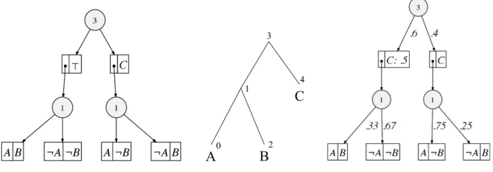
We will describe in the next section the approach we shall use for inducing probability distributions over structured spaces. This approach requires the Boolean formula defining the structured space to be in a tractable form, known as a sen-tential decision diagram(SDD) [Darwiche, 2011].1 Figure 1 depicts an example SDD for the Boolean formula
(A⇔B)∨((A⇔ ¬B)∧C).
A circle in an SDD is called adecision nodeand its children (paired boxes) are calledelements. Literals and constants (> and⊥) are called terminal nodes. For element (p, s), pis called aprimeandsis called asub. A decision nodenwith elements(p1, s1), . . . ,(pn, sn)is interpreted as(p1∧s1)∨ . . .∨(pn ∧sn). SDDs satisfy some strong properties that
make them tractable for certain tasks, such as probabilistic reasoning. For example, the prime and sub of an element do not share variables. Moreover, if (p1, s1), . . . ,(pn, sn) are
the elements of a decision node, then primesp1, . . . , pnmust
1
SDDs generalize OBDDs [Bryant, 1986] by branching on arbi-trary sentences instead of literals.
A
B
C
3 1 0 2 4Figure 1: An SDD, a vtree, and a PSDD for the Boolean formula(A⇔B)∨((A⇔ ¬B)∧C). form a partition (pi 6= false,pi∧pj = falsefori 6=j, and
p1∨. . .∨pn =true).
Each SDD is normalized for some vtree: a binary tree whose leaves are in one-to-one correspondence with the for-mula variables. The SDD of a Boolean forfor-mula is unique once a vtree is fixed. Figure 1 depicts an SDD and the vtree it is normalized for. More specifically, each SDD node is normalized for some vtree node. The root SDD node is nor-malized for the root vtree node. If a decision SDD node is normalized for a vtree nodev, then its primes are normalized for the left child ofv, and its subs are normalized for the right child ofv. As a result, terminal SDD nodes are normalized for leaf vtree nodes. Figure 1 labels decision SDD nodes with the vtree nodes they are normalized for.
In our experiments, we used the SDD package2to compile Boolean formulas, corresponding to total and partial ranking spaces, into SDDs.3 For partial ranking spaces, we report results onn = 64 items and t = 4 tiers, where each tier grows in size by a factor ofk, i.e., top-1, top-k, top-k2 and top-k3 items. To give a more comprehensive sense of space sizes, the following table shows the sizes of spaces and those of their SDD compilations, for variousnandk, fixingt= 4.
Size
n k SDD Structured Space Unstructured Space 8 2 443 840 1.84·1019 27 3 4,114 1.18·109 2.82·10219 64 4 23,497 3.56·1018 1.04·101233 125 5 94,616 3.45·1031 3.92·104703 216 6 297,295 1.57·1048 7.16·1014044 343 7 781,918 4.57·1068 7.55·1035415 The size of an SDD is obtained by summing the sizes of its decision nodes [Darwiche, 2011]. As we shall see in the next section, this size corresponds roughly to the number of
pa-2
Available athttp://reasoning.cs.ucla.edu/sdd/ 3
We did not use dynamic vtree search as provided by the SDD package. Instead, we used a static vtree, based on preliminary exper-imentation. Basically, for each positionj, we created a right-linear vtree over the variablesAij. We then composed these right-linear
vtrees together, also using a right-linear structure.
rameters needed to induce a distribution over the SDD mod-els. For example, for n = 64items, and tier growth rate k= 4, one needs about23,497parameters to induce a distri-bution over a structured space of size3.56·1018.
The SDDs for total rankings did not scale as well as they have a number of nodes that grows exponentially in the num-ber of itemsn(yet grows more slowly than the factorial func-tion). Hence, we were able to represent spaces for only a moderate number of items (about20), which is enough for certain datasets, such as the commonly used sushi dataset (consisting of 10 items). We will evaluate encodings for both total rankings and partial rankings (which scale better than total rankings), in our experiments.
4
Distributions over Structured Spaces
To induce a distribution over a structured space, we use prob-abilistic sentential decision diagrams(PSDDs) [Kisa et al., 2014]. According to this approach, the Boolean formula defining the structured space is first compiled into a normal-ized SDD. The SDD is then parameternormal-ized to induce a prob-ability distribution over its models. Figure 1 depicts an SDD and one of its parameterizations (PSDD).
An SDD is parameterized by providing distributions for its decision nodes and its terminal nodes, >. A decision SDD noden = (p1, s1), . . . ,(pk, sk)is parametrized using a
dis-tribution(θ1, . . . , θk), which leads to a decision PSDD node
(p1, s1, θ1), . . . ,(pk, sk, θk). The parametersθi are notated
on the edges outgoing from a decision node; see Figure 1. A terminal SDD noden=>is parameterized by a distribution (θ,1−θ), leading to terminal PSDD nodeX:θ. Here,X is the leaf vtree node thatnis normalized for; see Figure 1.
We will identify an SDD/PSDD with its root noder. More-over, ifnis a PSDD node, then[n]will denote the SDD that nparameterizes. That is, while nrepresents a probability distribution,[n]represents a Boolean formula. According to PSDD semantics, every PSDD noden, not just the rootr, induces a distributionPrnover the models of SDD[n].
The semantics of PSDDs is based on the notion of a con-text,γn, for PSDD noden. Intuitively, this is a Boolean
decision diagram will branch to noden. We will not describe the distribution Prr induced by a PSDD r, but will stress
the following local semantics of PSDD parameters. For a decision PSDD noden = ((p1, s1, θ1), . . . ,(pk, sk, θk), we
havePrr(pi|γn) = θi. Moreover, for a terminal SDD node
n = X:θ, we have Prr(X|γn) = θ. This local
seman-tics of PSDD parameters is the key reason behind their many well-behaved properties (e.g., the existence of closed-form maximum-likelihood parameter estimates for complete data). We defer the reader to Kisaet al.[2014] for a thorough expo-sition of PSDD syntax, semantics and properties.
5
Querying with Constraints
Suppose now that we have a probability distributionPr and we want to compute the probability of a Boolean formula α. For example, Pr can be a distribution over preferences in movies, andαcould represent “a comedy appears as one of the top-10 highest ranked movies.” We may also be inter-ested inPr(.|α), which is the conditional distribution over rankings, assuming that a comedy appears in the top-10.
The ability to reason about arbitrary constraints is a pow-erful one. For example, it allows one to diversify recommen-dations in preference-based reasoning, as we discuss later. In most representations, this ability is either not present, or it is intractable. For example, in a Bayesian network, one can use the method of virtual evidence [Pearl, 1988; Mateescu and Dechter, 2008], to represent a logical con-straint. However, this will in general lead to a highly-connected network, making inference intractable.
A key technical contribution of this paper is an observation that the probability of a Boolean formula can be computed efficiently, in a distribution induced by a PSDD, given that the formula is represented by an SDD with the same vtree as the PSDD.4
Theorem 1. Suppose we have a PSDDnwith distribution
Prnand sizesn, and a Boolean formulaαrepresented by an
SDDmof sizesm. If SDDmhas the same vtree as PSDDn,
thenPrn(α)can be computed in timeO(snsm).5
Suppose that PSDDnhas elements(pi, si, θi)and SDDα
has elements(qj, rj).Our approach for computing the
prob-ability of αis based on the following recurrence, which is implemented by Algorithm 1: Prn(α) = X j Prn(qj∧rj) =X i X j Prpi(qj)·Prsi(rj)·θi 4
This assumption, that the SDD and PSDD share the same vtree, is key to the efficiency of computing the probability of a Boolean constraint. Otherwise, the problem becomes NP-hard, which fol-lows from the hardness of conjoining two OBDDs that respect two different orders [Meinel and Theobald, 1998; Darwiche and Mar-quis, 2002].
5
This is a loose upper bound. A more accurate bound is
P
vsv,nsv,m, where vis a non-leaf vtree node, sv,m is the size
of decision PSDD nodes normalized forv, andsv,mis the size of
decision SDD nodes normalized forv.
Algorithm 1pr-constraint(n, m)
input:A PSDDninducing distributionPrnand an SDDm
representing Boolean formulaα. The PSDD and SDD respect the same vtree.
output:Prn(α).
main:
1: if(n, m)∈cachethen
2: return cache[(n, m)]
3: else ifnis a decision nodethen 4: ρ←0
5: foreach element(pi, si, θi)in PSDDndo
6: foreach element(qj, rj)in SDDmdo
7: ρleft←pr-constraint(pi, qj)
8: ρright←pr-constraint(si, rj)
9: ρ←ρ+ρleft·ρright·θi
10: cache[(n, m)] =ρ
11: return ρ
12: else{// n and m are terminals}
13: if[n]∧misfalsethen
14: return 0
15: else if[n]∧mistruethen
16: return 1
17: else if[n]is a literalthen
18: return 0if[n]∧misfalse, otherwise 1
19: else ifnis a terminalX:θX, andmis a literalthen
20: return θXifmisX, or1−θXifmis¬X
In a second pass on the PSDD and SDD, we can compute the marginalsPr(X |α)for each variableX, as well as the probabilities of non-root SDD nodes. This is analogous to the two-pass algorithm given in Kisaet al.[2014]. This ability to compute marginals enables an EM algorithm for PSDDs, which we discuss next.
6
Learning from Constraints
Kisaet al.[2014] provided an algorithm for learning the pa-rameters of a PSDD given acompletedataset. This algorithm identified the (unique) maximum likelihood parameters, and further, in closed-form. We will now present our second, main technical contribution: An efficient algorithm for learn-ing the parameters of a PSDD given anincompletedataset.
We start first with some basic definitions. An instantiation ofallvariables is acomplete example,while an instantiation ofsomevariables is anexample. There are2n distinct
com-plete examples overnvariables, and3ndistinct examples. A complete dataset is a multi-set of complete examples (i.e., a complete example may appear multiple times in a dataset). Moreover, traditionally, an incomplete dataset is defined as a multi-set of examples. One can view an example as a set of complete examples (those consistent with the example). Hence, we will use a more general definition of an incomplete dataset, defined as a multi-set of Boolean formulas, with each formula corresponding to a set of complete examples (those consistent with the formula). This definition is too general to appear practical. However, as we shall show, if we represent these Boolean formulas (i.e., examples) as SDDs, then
The-orem 1 allows us to efficiently learn parameters from such datasets. We will next provide an EM algorithm for this pur-pose, which has a polytime complexity per iteration.
Given a PSDD structure, and an incomplete dataset spec-ified as a set of SDDs, our goal is to learn the value of each PSDD parameter. More precisely, we wish to learnmaximum likelihoodparameters: ones that maximize the probability of examples in the dataset. LetPrθdenote the distribution
in-duced by the PSDD structure and parametersθ. Thelog like-lihoodof these parameters given a datasetDis defined as
LL(θ|D) =
N
X
i=1
logPrθ(Di),
where Di ranges over all N examples of our dataset D.
Again, eachDi is an SDD, whose probability Prθ(Di)can
be computed using Algorithm 1. Our goal is then to find the maximum likelihood parameters
θ?= argmax
θ
LL(θ|D).
For an incomplete dataset, finding the globally optimal pa-rameter estimates may not be tractable. Instead, we can more simply search for stationary points of the log likelihood, i.e., points where the gradient is zero (any global optimum is a stationary point, but not vice-versa). Such points are charac-terized by the following theorem.
Theorem 2. Let Dbe an incomplete dataset, and letθ be
the parameters of a corresponding PSDD with distribution
Prθ. Parametersθare a stationary point of the log likelihood
LL(θ|D)(subject to normalization constraints on θ) iff for each PSDD nodenwith contextγn:
– Ifnis a decision node with elements(pi, si, θi), then:
θi=
PN
i=1Prθ(pi, γn| Di)
PN
i=1Prθ(γn| Di)
– Ifnis a terminal nodeX:θX, then:
θX= PN i=1Prθ(X, γn| Di) PN i=1Prθ(γn| Di) .
This theorem suggests an iterative EM algorithm for find-ing stationary points of the log likelihood. First, we start with some initial parameter estimates θ0 at iterationt = 0. For iterationt >0, we use the above update to compute parame-tersθtgiven the parametersθt−1from the previous iteration. When the parameters of one iteration do not change in the next (in practice, up to some threshold), we say that the itera-tions have converged to a fixed point.
An iteration of the proposed algorithm is implemented by traversing the dataset, while applying Algorithm 1 to each example (i.e., SDD) and the current PSDD. This is sufficient to obtain the quantities needed by the update equations. For a dataset withmdistinct examples, the proposed algorithm will therefore apply Algorithm 1 a total ofmtimes per iteration, leading to a polytime complexity per iteration. We can show that the proposed algorithm is indeed an EM algorithm by
0 5 10 15 20 # of mixture components −14.4 −14.3 −14.2 −14.1 −14.0 −13.9 −13.8 −13.7 −13.6 av er age log-lik elihood sushi mix-of-mallows psdd
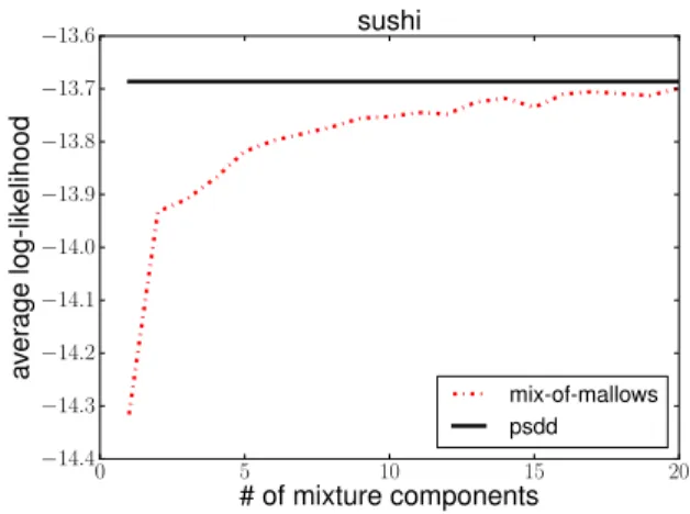
Figure 2: Mallows Mixture Model vs PSDDs showing that it obtains the same updates obtained by the fol-lowing algorithm. First, we “complete” the dataset by replac-ing each SDD example by the complete examples consistent with it. Second, we compute the probability of each complete example using the current PSDD. Finally, we use the closed forms in [Kisaet al., 2014] to obtain the next parameter esti-mates based on the completed data. The same proof technique is used in Darwiche [2009] and Koller and Friedman [2009] for justifying the EM algorithm for Bayesian networks.
7
Experiments
We now empirically evaluate the PSDD as a model for pref-erence distributions. We first evaluate the encoding for total rankings, where we highlight (a) the quality of learned mod-els and (b) the utility of PSDDs in terms of its query capabil-ities. We also evaluate the more scalable encoding for partial rankings and further demonstrate (c) the capabilities that PS-DDs provide, in particular for diversified recommendations.
7.1
Total Rankings
Consider thesushidataset, which consists of 5,000total rankings of10 different types of sushi [Kamishima, 2003]. We learned a PSDD from the full dataset, using the encod-ing for total rankencod-ings, and analyzed the resultencod-ing model. A dataset composed of total rankings is a complete dataset, so we use the closed forms of Kisaet al., 2014 to estimate the maximum likelihood parameters of a PSDD. The correspond-ing PSDD required4,097(independent) parameters. We fur-ther assumed a Dirichlet prior with exponents2, which corre-sponds to Laplace smoothing.
Quality of Learned Model.We compared the learned PSDD
model for thesushi dataset with a learned Mallows mix-ture model. As performed by Lu and Boutilier [2011], we first split the dataset into a training set of 3,500 instances, and a test set of 1,500 instances. From the training set, we learned a single PSDD model and 10 Mallows mixture mod-els using EM.6In Figure 2, we compare the PSDD and
Mal-6
For the Mallows mixture model, we used the implementation of Lu and Boutilier [2011] with default settings.
lows mixture models in terms of (average) log likelihood of the test set, for an increasing number of mixture components (for the Mallows model). We see that the PSDD dominates the Mallows model for all numbers of mixture components that were evaluated (up to 20, as in Lu and Boutilier [2011]). This suggests that PSDDs are expressive, and better capable of representing distributions such as the one underlying the
sushidataset. This is in contrast to the popular Mallows
models (and their mixtures), whose underlying assumptions are relatively strong (i.e., that there exists a central ranking).
Query Capabilities. Once a model is learned, PSDDs
ad-mit a variety of queries. For example, we can compute the most likely total rankingσ?= argmax
σPr(σ),which
corre-sponds to the most probable explanation (MPE) in Bayesian networks. We can also compute the expected rank of each itemi:
E[j] =X
j
j·Pr(Aij).
Moreover, using Theorem 1, it is possible to predict a pair-wise preferencei > j, given a pairwise preferencek > l. In particular, we are interested inPr(i > j |k > l), which is the probability of a preferencei > jgiven the preference k > l. We enumerated all such combinations ofi, j, kandl, wherei, j, k, lare pairwise distinct, and examined in particu-lar the log odds change, i.e.,
logF(i > j|k > l) = logO(i > j|k > l)−logO(i > j) where we have the odds
O(α) = Pr(α) 1−Pr(α),
for an eventα; for more on log-odds change, see, e.g., Chan and Darwiche [2005]. A large log-odds change indicates a large increase in a pairwise preferencei > jgiven the pref-erence k > l. In our PSDD, the greatest log-odds change was:
logF(egg>fatty tuna|cucumber roll>tuna) = 1.295 where the odds of preferring egg to fatty tuna increased from 0.238to0.868when cucumber rolls are preferred to tuna.
7.2
Partial Rankings
Consider now themovielensdataset,7 which consists of over 1 million ratings of approximately 3,900 movies and 6,040 users. Here, each rating is an integer from 1 to 5, in contrast to the total orderings given in the sushidataset. Following Lu and Boutilier [2011], we extracted from these ratings a set of pairwise preferences for each user. In this case, our dataset is incomplete, and we utilized the EM algo-rithm for PSDDs that we proposed in this paper.
We employ our encoding of partial rankings for this eval-uation. In particular, we extract the top 64 most frequently rated movies from themovielensdataset, and use the rat-ings of the resulting 5,891 of 6,040 users who rated at least one of these movies.8 For each user, we construct an SDD
7
Available athttp://grouplens.org/ 8
Lu and Boutilier [2011] extract the 200 most frequently rated movies. We retain only 64 movies due to time considerations.
representing their pairwise preferences, based on their rat-ings. In particular, if a user gives movie i a higher rating than another moviej, we assert a constraint that the movie is at least as highly ranked as the other (or appears in at least as high a tier), i.e., i≥j. We obtain an SDD for each user by conjoining together all such pairwise preferences (the average size of a user SDD was in the tens of thousands). For partial rankings of 64 movies, we assume four tiers representing the top-1, top-5, top-25 and top-64 movies. The corresponding PSDD has18,711(independent) parameters. We finally run EM on the PSDD for 5 iterations. We also use the system of Lu and Boutilier [2011] to learn the Mallows model from pairwise constraints.
Total versus Partial Ranking Models.A comparison with a
Mallows models in terms of likelihoods is not possible here as the two models are quite different in scope: one is modeling a distribution over total rankings, while the other is modeling a distribution over partial rankings. We were curious, however, to see the extent to which these models agreed on recommen-dations. Our general observation has been that they come out close. For example, the central ranking obtained by a Mal-lows model, and the sorted list of expected rankings given by the PSDD model, agreed on the top10movies (but disagreed somewhat on their order). We omit the details of this and other examples here, however, due to space limitations.
Query Capabilities. We will now illustrate some further
queries that are permitted by the proposed framework. Most current frameworks for preference distributions cannot han-dle such queries exactly and efficiently.
First, we may ask for the top-5 movies (by expected tier), given the constraintα: “the highest ranked movie is Star Wars V” (which we encode as an SDD and use as evidence):
1 Star Wars: Episode V - The Empire Strikes Back (1980) 2 Star Wars: Episode IV - A New Hope (1977)
3 Godfather, The (1972)
4 Shawshank Redemption, The (1994) 5 Usual Suspects, The (1995)
We see that another Star Wars movie is also highly ranked. However, if we wanted to use this information to recommend a movie to a user, whose favorite movie was Star Wars V, a recommendation of Star Wars IV would not be particularly useful (as having seen Star Wars V likely implies that one has seen the prequel Star Wars IV as well). We could condition on an additional constraintβ, that “no other Star Wars movie appears in the top-5.” Going further still, we could assert a third constraintγ, that “at least one comedy appears in the top-5.” Conditioning on these three constraintsα, β andγ, we obtain the new ranking:
1 Star Wars: Episode V - The Empire Strikes Back (1980) 2 American Beauty (1999)
3 Godfather, The (1972) 4 Usual Suspects, The (1995) 5 Shawshank Redemption, The (1994)
Here, the movie Star Wars IV was replaced by the com-edy/drama American Beauty. This provides an illustration of the powerful, and open ended, type of queries permitted by the proposed framework.
8
Conclusion and Related Work
We have introduced a general framework for probabilistic preference learning. Our aim was to provide a different per-spective on preference learning, rooted in the recent devel-opments on learning structured probability spaces [Kisa et al., 2014] and the tractable learning paradigm [Domingos and Lowd, 2014]. To support the preference learning application, we extended PSDDs to reason with structured queries and to learn from incomplete structured data. We were particu-larly motivated by the need to support heterogeneous data, and complex queries, such as diversified recommendations.
Existing work on preference distributions has focused on two representations of historical significance, namely the Plackett-Luce [Plackett, 1975; Luce, 1959] and Mal-lows [1957] model, and extensions thereof [Fligner and Ver-ducci, 1986; Murphy and Martin, 2003; Meila and Chen, 2010]. Although these models were successfully applied in several applications, they can also be restrictive. As a repre-sentation, for example, the Mallows model and its extensions encode the distance from a (small) number of consensus rank-ings, limiting the number of modes in the distribution. Com-pact representations of preferences distributions are also pur-sued by Huanget al.[2009] and Huang and Guestrin [2009]. These are sophisticated and dedicated representation of per-mutations. Moreover, they either do not support tractable ex-act inference, or all the types of rank data considered here.
The PSDD representation is founded on a long tradition of tractable representations of logical knowledge bases in knowledge compilation [Darwiche and Marquis, 2002]. It is also related to other tractable probabilistic representations, such as sum-product networks, which exploit similar proper-ties for efficient learning [Peharzet al., 2014].
We finally note that the need for diversity (as in diversified recommendations) has been recognized before [McNeeet al., 2006; Sanneret al., 2011; Heet al., 2012]. Similar observa-tions have also been stated for recommender systems [Rashid
et al., 2002] and matching problems [Charlinet al., 2012].
Acknowledgments
We thank Tyler Lu and Craig Boutilier for providing their system for Mallows mixture models, and Scott Sanner for commenting on an earlier draft of this paper. This work was supported by ONR grant #N00014-12-1-0423, NSF grant #IIS-1118122, and the Research Foundation-Flanders (FWO-Vlaanderen). Guy Van den Broeck is also affiliated with KU Leuven, Belgium.
References
[Bryant, 1986] R. E. Bryant. Graph-based algorithms for Boolean function manipulation. IEEE Transactions on Computers, C-35:677–691, 1986.
[Burges, 2010] Christopher J.C. Burges. From RankNet to Lamb-daRank to LambdaMART: An overview. 11:23–581, 2010. [Busseet al., 2007] Ludwig M Busse, Peter Orbanz, and
Joachim M Buhmann. Cluster analysis of heterogeneous rank data. InProceedings of ICML, pages 113–120. ACM, 2007.
[Chan and Darwiche, 2005] Hei Chan and Adnan Darwiche. On the revision of probabilistic beliefs using uncertain evidence. Artifi-cial Intelligence, 163:67–90, 2005.
[Charlinet al., 2012] Laurent Charlin, Craig Boutilier, and Richard S Zemel. Active learning for matching problems. In
Proceedings of ICML, pages 337–344, 2012.
[Collins and Koo, 2005] Michael Collins and Terry Koo. Discrim-inative reranking for natural language parsing. Computational Linguistics, 31(1):25–70, 2005.
[Darwiche and Marquis, 2002] Adnan Darwiche and Pierre Mar-quis. A knowledge compilation map.JAIR, 17:229–264, 2002. [Darwiche, 2009] Adnan Darwiche. Modeling and Reasoning with
Bayesian Networks. Cambridge University Press, 2009. [Darwiche, 2011] Adnan Darwiche. SDD: A new canonical
repre-sentation of propositional knowledge bases. InProceedings of IJCAI, pages 819–826, 2011.
[Dempsteret al., 1977] A.P. Dempster, N.M. Laird, and D.B. Ru-bin. Maximum likelihood from incomplete data via the EM algo-rithm.Journal of the Royal Statistical Society B, 39:1–38, 1977. [Doignonet al., 2004] J. Doignon, A. Pekeˇc, and M. Regenwetter. The repeated insertion model for rankings: Missing link between two subset choice models.Psychometrika, 69(1):33–54, 2004. [Domingos and Lowd, 2014] Pedro Domingos and Daniel Lowd.
Learning tractable probabilistic models. UAI Tutorial, 2014. [Dworket al., 2001] Cynthia Dwork, Ravi Kumar, Moni Naor, and
Dandapani Sivakumar. Rank aggregation methods for the web. InProceedings of WWW, pages 613–622. ACM, 2001.
[Fligner and Verducci, 1986] Michael A Fligner and Joseph S Ver-ducci. Distance based ranking models.Journal of the Royal Sta-tistical Society. Series B (Methodological), pages 359–369, 1986. [Guiver and Snelson, 2009] J. Guiver and E. Snelson. Bayesian in-ference for plackett-luce ranking models. InProc. of ICML, 2009. [Heet al., 2012] J. He, H. Tong, Q. Mei, and B. Szymanski. Gen-DeR: A generic diversified ranking algorithm. InAdvances in Neural Information Processing Systems 25, pages 1142–1150, 2012.
[Huang and Guestrin, 2009] Jonathan Huang and Carlos Guestrin. Riffled independence for ranked data. InAdvances in Neural Information Processing Systems, pages 799–807, 2009. [Huanget al., 2009] J. Huang, C. Guestrin, and L. Guibas. Fourier
theoretic probabilistic inference over permutations. The Journal of Machine Learning Research, 10:997–1070, 2009.
[H¨ullermeieret al., 2008] E. H¨ullermeier, J. F¨urnkranz, W. Cheng, and K. Brinker. Label ranking by learning pairwise preferences.
Artificial Intelligence, 172(16):1897–1916, 2008.
[Hunter, 2004] David R Hunter. Mm algorithms for generalized bradley-terry models.Annals of Statistics, pages 384–406, 2004. [Kamishima, 2003] Toshihiro Kamishima. Nantonac collaborative filtering: recommendation based on order responses. In Proceed-ings KDD, pages 583–588, 2003.
[Karatzoglouet al., 2013] Alexandros Karatzoglou, Linas Bal-trunas, and Yue Shi. Learning to rank for recommender systems. InProceedings of the 7th ACM conference on Recommender sys-tems, pages 493–494. ACM, 2013.
[Kisaet al., 2014] D. Kisa, G. Van den Broeck, A. Choi, and A. Darwiche. Probabilistic sentential decision diagrams. In Pro-ceedings of KR, 2014.
[Koller and Friedman, 2009] D. Koller and N. Friedman. Prob-abilistic Graphical Models: Principles and Techniques. MIT Press, 2009.
[Lauritzen, 1995] S. L. Lauritzen. The EM algorithm for graphical association models with missing data. Computational Statistics and Data Analysis, 19:191–201, 1995.
[Lebanon and Mao, 2007] Guy Lebanon and Yi Mao. Non-parametric modeling of partially ranked data. In Advances in neural information processing systems, pages 857–864, 2007. [Liu, 2009] Tie-Yan Liu. Learning to rank for information retrieval.
Foundations and Trends in Information Retrieval, 3(3), 2009. [Lu and Boutilier, 2011] Tyler Lu and Craig Boutilier. Learning
Mallows models with pairwise preferences. InProceedings of ICML, pages 145–152, 2011.
[Luce, 1959] R Duncan Luce. Individual choice behavior: A theo-retical analysis. Wiley, 1959.
[Mallows, 1957] Colin L. Mallows. Non-null ranking models.
Biometrika, 1957.
[Marden, 1996] John I. Marden. Analyzing and modeling rank data. CRC Press, 1996.
[Mateescu and Dechter, 2008] Robert Mateescu and Rina Dechter. Mixed deterministic and probabilistic networks.Annals of Math-ematics and AI, 54(1-3):3–51, 2008.
[McNeeet al., 2006] Sean M. McNee, John Riedl, and Joseph A. Konstan. Being accurate is not enough: how accuracy metrics have hurt recommender systems. InProceedings of CHI, pages 1097–1101, 2006.
[Meila and Chen, 2010] Marina Meila and Harr Chen. Dirichlet process mixtures of generalized mallows models. InProceedings of UAI, 2010.
[Meilaet al., 2007] Marina Meila, Kapil Phadnis, Arthur Patterson, and Jeff A. Bilmes. Consensus ranking under the exponential model. InProceedings of UAI, pages 285–294, 2007.
[Meinel and Theobald, 1998] Christoph Meinel and Thorsten Theobald. Algorithms and Data Structures in VLSI Design: OBDD — Foundations and Applications. Springer, 1998. [Murphy and Martin, 2003] Thomas Brendan Murphy and Donal
Martin. Mixtures of distance-based models for ranking data.
Computational statistics & data analysis, 41(3):645–655, 2003. [Pearl, 1988] J. Pearl. Probabilistic Reasoning in Intelligent
Sys-tems: Networks of Plausible Inference. Morgan Kaufmann, 1988. [Peharzet al., 2014] R. Peharz, R. Gens, and P. Domingos. Learn-ing selective sum-product networks. InLTPM workshop, 2014. [Plackett, 1975] Robin L Plackett. The analysis of permutations.
Applied Statistics, pages 193–202, 1975.
[Rashidet al., 2002] A. M. Rashid, I. Albert, D. Cosley, S. K. Lam, S. M. McNee, J. A. Konstan, and J. Riedl. Getting to know you: learning new user preferences in recommender systems. In Pro-ceedings of IUI, pages 127–134, 2002.
[Sanneret al., 2011] S. Sanner, S. Guo, T. Graepel, S. Kharazmi, and S. Karimi. Diverse retrieval via greedy optimization of ex-pected 1-call@k in a latent subtopic relevance model. In Pro-ceedings of CIKM, pages 1977–1980, 2011.
[Vembu and G¨artner, 2011] S. Vembu and T. G¨artner. Label rank-ing algorithms: A survey. InPreference learning, pages 45–64. Springer, 2011.
[Young, 1995] Peyton Young. Optimal voting rules.The Journal of Economic Perspectives, pages 51–64, 1995.