Nonlinear IV unit root tests in panels with
cross-sectional dependency
Yoosoon Chang
∗Department of Economics-MS22, Rice University, 6100 Main Street, Houston, TX 77005-1892, USA
Abstract
We propose a unit root test for panels with cross-sectional dependency. We allow general de-pendency structure among the innovations that generate data for each of the cross-sectional units. Each unit may have di)erent sample size, and therefore unbalanced panels are also permitted in our framework. Yet, the test is asymptotically normal, and does not require any tabulation of the critical values. Our test is based on nonlinear IV estimation of the usual augmented Dickey–Fuller type regression for each cross-sectional unit, using as instruments nonlinear transformations of the lagged levels. The actual test statistic is simply de2ned as a standardized sum of individual IV t-ratios. We show in the paper that such a standardized sum of individual IV t-ratios has limit normal distribution as long as the panels have large individual time series observations and are asymptotically balanced in a very weak sense. We may have the number of cross-sectional units arbitrarily small or large. In particular, the usual sequential asymptotics, upon which most of the available asymptotic theories for panel unit root models heavily rely, are not required. Finite sample performance of our test is examined via a set of simulations, and compared with those of other commonly used panel unit root tests. Our test generally performs better than the existing tests in terms of both 2nite sample sizes and powers. We apply our nonlinear IV method to test for the purchasing power parity hypothesis in panels.
c
2002 Elsevier Science B.V. All rights reserved. JEL classi'cation:C1; C15; C32; C33
Keywords:Panels with cross-sectional dependency; Unit root tests; Nonlinear instruments; Average IV
t-ratio statistics
1. Introduction
It is now widely perceived that the panel unit root test is important. The test helps us to answer some of the important economic questions like growth convergence and
∗Corresponding author. Tel.: +713-348-2796; fax: +713-348-5278.
E-mail address:[email protected] (Yoosoon Chang).
0304-4076/02/$ - see front matter c2002 Elsevier Science B.V. All rights reserved. PII: S 0304-4076(02)00095-7
divergence, and purchasing power parity (PPP), among many others. Moreover, it also provides a means to improve the power of the unit root test, which is known to often yield very low discriminatory power if performed on individual time series. A number of unit root tests for panel data are now available in the literature. Examples include the tests proposed by Levin et al. (1997), Im et al. (1997), Maddala and Wu (1999), Choi (2001) and Chang (2000). The reader is referred to Banerjee (1999) for some detailed discussions on the existing panel unit root tests and other related issues.
Rather unsatisfactorily, however, most existing panel unit root tests assume cross-sectional independence, which is quite restrictive given the nature of economic panel data. Such tests are, of course, likely to yield biased results if applied to the panels with cross-sectional dependency. Maddala and Wu (1999) conduct a set of simulations to evaluate the performances of the commonly used panel unit root tests that are developed under the cross-sectional independence when in fact the panel is spatially dependent. They, in particular, show that the panel unit root tests based on independence across cross-sectional units, such as those considered in Levin et al. (1997) and Im et al. (1997), perform poorly for cross-sectionally correlated panels.
The cross-sectional dependency is very hard to deal with in nonstationary panels. In the presence of cross-sectional dependency, the usual Wald type unit root tests based upon the OLS and GLS system estimators have limit distributions that are dependent in a very complicated way upon various nuisance parameters de2ning correlations across individual units. There does not exist any simple way to eliminate the nuisance para-meters in such systems. This was shown in Chang (2000). None of the existing tests, except for Chang (2000) which relies on the bootstrap method, successfully overcomes the nuisance parameter problem in panels with cross-sectional dependence.
In this paper, we take the IV approach to solve the nuisance parameter problem for the unit root test in panels with cross-sectional dependency. Our approach here is based upon nonlinear IV estimation of the autoregressive coeHcient. We 2rst estimate the AR coeHcient from the usual augmented Dickey–Fuller (ADF) regression for each cross-sectional unit using the instruments generated by an integrable transformation of the given time series. We then construct the t-ratio statistic for testing the unit root based on the nonlinear IV estimator for the AR coeHcient. We show for each cross-sectional unit that such nonlinear IV t-ratio statistic for testing the unit root has limiting standard normal distribution under the null hypothesis, just as in the stationary alternative cases. The asymptotic normality under the null indeed establishes continuity of the limit theory for thet-statistic over the entire parameter space covering both null and alternative hypotheses. This clearly makes a drastic contrast with the limit theory of the standard t-statistic based on the ordinary least-squares estimator.
More importantly, we show that the individual IV t-ratio statistics are asymptoti-cally independent even across dependent cross-sectional units. The cross-sectional in-dependence of the individual IV t-ratio statistics follows readily from the asymptotic orthogonality for the nonlinear transformations of integrated processes by an integrable function, which is established in Chang et al. (2001). We are therefore led to consider the average of these independent individual IVt-ratio statistics as a statistic for testing joint unit root null hypothesis for the entire panel. The actual test statistic is simply de2ned as a standardized sum of the individual IVt-ratios. We show in the paper that
such a normalized sum of the individual IV t-ratios has standard normal limit distri-bution as long as Tmin → ∞ andTmax1=4 logTmax=Tmin3=4→0, where Tmin and Tmax denote,
respectively, the minimum and maximum numbers of the time series observations Ti’s
for the cross-sectional unitsi= 1; : : : ; N. The usual sequential asymptotics, upon which most of the available asymptotic theories for panel unit root models heavily rely, are therefore not required. We may thus allow the number of cross-sectional units to be arbitrarily small or large.1 Our test is applicable for all panels that have large num-bers of individual time series observations and are asymptotically balanced in the sense mentioned above.
Finite sample performance of our average IV t-ratio statistic, which we call SN
statistic, is examined via a set of simulations, and compared with that of the commonly used average statistict-bar by Im et al. (1997). Our test generally performs better than thet-bar test in terms of both 2nite sample sizes and powers. The simulations conducted indeed corroborate the standard normal limit theory we provide here. The 2nite sample sizes ofSN are computed using the standard normal critical values, and shown to very
well approximate the nominal sizes. This is quite contrary to the well-known 2nite sample size distortions of the t-bar test, see Maddala and Wu (1999) for example. The discriminatory powers ofSN are yet noticeably higher than the t-bar test. We also
apply our nonlinear IV method to test for the PPP hypothesis using the data sets from Papell (1997) and Oh (1996). Our test SN supports strongly the PPP relationships,
contrary to most of the previous empirical 2ndings which are usually inconclusive. The rest of the paper is organized as follows. Section 2 introduces the model, as-sumptions and background theory. Section 3 presents the nonlinear IV estimation of the augmented autoregression and derives the limit theory for the nonlinear IVt-ratio statistics for each cross-sectional unit. In Section 4, we introduce a nonlinear IV panel unit root test and establish its limit theory. It is, in particular, shown that the test is asymptotically standard normal. Section 5 extends our nonlinear IV methodology to models with deterministic components such as constant and linear time trend. In Section 6, we conduct simulations to investigate 2nite sample performance of the av-erage IV t-ratio statistic. Section 7 provides empirical illustrations for testing the PPP using our nonlinear panel IV unit root test. Section 8 concludes, and mathematical proofs are provided in the Appendix.
2. Model, assumptions and background theory
We consider a panel model generated as the following 2rst-order autoregressive regression:
yit=iyi;t−1+uit; i= 1; : : : ; N; t= 1; : : : ; Ti: (1)
As usual, the indexidenotes individual cross-sectional units, such as individuals, house-holds, industries or countries, and the index t denotes time periods. The number of time series observationsTi for each individuali may di)er across cross-sectional units.
Hence, unbalanced panels are allowed in our model. We are interested in testing the unit root null hypothesis, i = 1 for all yit given as in (1), against the alternative,
|i|¡1 for some yit; i= 1; : : : ; N. Thus, the null implies that all yit’s have unit roots,
and is rejected if any one of yit’s is stationary with |i|¡1. The rejection of the
null therefore does not imply that the entire panel is stationary. The initial values (y10; : : : ; yN0) of (y1t; : : : ; yNt) do not a)ect our subsequent asymptotic analysis as long
as they are stochastically bounded, and therefore we set them at zero for expositional brevity.
It is assumed that the error term uit in model (1) is given by an AR(pi) process
speci2ed as
i(L)u
it=it; (2)
whereL is the usual lag operator and
i(z) = 1−pi k=1
i;kzk
for i= 1; : : : ; N. Note that we let i(z) and p
i (which is assumed to be 2xed) vary
across i, thereby allowing heterogeneity in individual serial correlation structures. We assume:
Assumption 2.1. For i= 1; : : : ; N; i(z)= 0 for all |z|61.
Under Assumption 2.1, the AR(pi) process uit is invertible, and has a
moving-average representation
uit=i(L)it;
wherei(z) =i(z)−1 and is given by
i(z) = ∞
k=0
i;kzk:
We allow for the cross-sectional dependency through the cross-correlation of the in-novations it; i= 1; : : : ; N, that generate the errors uit’s. To de2ne the cross-sectional
dependency more explicitly, we de2ne (t)Tt=1 by
t= (1t; : : : ; Nt) (3)
and denote by | · | the Euclidean norm: for a vector x= (xi); |x|2=ix2i, and for a
matrixA= (aij); |A|=i;ja2ij. The data generating process for the innovations (t) is
assumed to satisfy the following assumption.
Assumption 2.2. (t) is an iid (0; ) sequence of random variables with E|t|‘¡∞
for some‘ ¿4; and its distribution is absolutely continuous with respect to Lebesgue measure and has characteristic function ’ such that lim→∞||r’() = 0; for some r ¿0.
Assumption 2.2 is strong, but is still satis2ed by a wide class of data generating processes including all invertible Gaussian ARMA models. Note that here the errors are
assumed to be iid across time periods. However, they are allowed to be cross-sectionally dependent. The technical assumption on the characteristic function is required for our subsequent asymptotics on nonlinear functions of integrated processes as used in Park and Phillips (1999, 2001).
De2ne a stochastic processesUT for t as
UT(r) =T−1=2
[Tr]
t=1
t
on [0;1], where [s] denotes the largest integer not exceeding s. The process UT(r)
takes values in D[0;1]N, where D[0;1] is the space of cadlag functions on [0;1].
Under Assumption 2.2, an invariance principle holds for UT, viz.,
UT →dU (4)
as T → ∞, where U is an N-dimensional vector Brownian motion with covariance matrix . It is also convenient to de2ne BT(r) from ut = (u1t; : : : ; uNt), similarly as
UT(r). Then we have BT →d B, where B= (B1; : : : ; BN) and Bi=i(1)Ui. This is
shown in Phillips and Solo (1992).
Our theory relies heavily on the local time of Brownian motion as in Park and Phillips (1999, 2001), Chang and Park (1999) and Chang et al. (2001). The reader is referred to these papers and the references cited there for the concept of local time and its use in the asymptotics for nonlinear models with integrated time series. To de2ne local times that appear in our limit theory more precisely, we 2rst write the limit vector Brownian motion given in (4) explicitly as U(r) = (U1(r); : : : ; UN(r)). We denote by
Li the (scaled) local time of Ui, for i= 1; : : : ; N, which is de2ned by
Li(t; s) = lim j→0 1 2j t 0 1{|Ui(r)−s|¡j}dr:
The local time Li is therefore the time that the Brownian motion Ui spends in the
neighborhood ofs, upto timet, measured in chronological units.2 Then we may have an important relationship
t
0 G(Ui(r)) dr=
∞
−∞G(s)Li(t; s) ds (5)
which we refer to as the occupation times formula.
In addition to the Brownian motions U= (U1; : : : ; UN), we need to introduce
an-other set of standard Brownian motionsW= (W1; : : : ; WN). Throughout the paper, the
Brownian motion W will be assumed to be standard vector Brownian motion that is independent of U.
We now introduce the class of regularly integrable transformations in R, which plays an important role in the subsequent development of our theory.
2Usually, the local time is de2ned in units of quadratic variation time. Therefore, the local timeLU
iofUi de2ned in the usual manner is given byLUi=#2iLi in terms of our local timeLi, where#2i is the variance
Denition 2.3. A transformation G on R is said to be regularly integrable if G is a bounded integrable function such that for some constants c ¿0 and k ¿6=(‘−2) with ‘ ¿4 given in Assumption 2.2; |G(x)−G(y)|6c|x−y|k on each piece A
i of
its supportA=mi=1 Ai⊂R.
The regularly integrable transformations are roughly integrable functions that are reasonably smooth on each piece of their supports. The required smoothness depends on the moment condition of the innovation sequence (t). Let‘ be the maximum order
of the existing moments. If ‘ ¿8, any piecewise Lipschitz continuous function is allowed. For the indicator function on a compact interval to be regularly integrable, on the other hand, it is suHcient to have ‘ ¿4. The de2nition of the regularly integrable function in De2nition 2.3 is identical to the one introduced in Park and Phillips (1999, 2001).
The asymptotic behaviors of the nonlinear functions of an integrated time series are analyzed by Park and Phillips (1999, 2001). For (yit) generated as in (1), they provide,
in particular, the asymptotic theories for the sample moments given by Ti
t=1 G(yit)
and Ti
t=1 G(yi;t−1)it, which are referred to in their paper as the mean and covari-ance asymptotics, respectively, for various types of function G. Our subsequent theory is based upon the mean and covariance asymptotics for G regularly integrable. The conditions in Assumption 2.2 are required to obtain the relevant asymptotics. They are stronger than those required for the usual unit root asymptotics, because we need the convergence and invariance of the sample local time, as well as those of the sample Brownian motion, for the asymptotics of integrable transformations of integrated time series.
We now obtain the Beveridge–Nelson representations foruit andyit. Leti(1) = 1−
pi
k=1 i;k. Then it is indeed easy to get
uit=i1(1)it+ pi k=1 pi j=k i;j i(1) (ui;t−k−ui;t−k+1) =i(1)it+ ( ˜ui;t−1−u˜it);
where i(1) = 1=i(1) and ˜uit =pk=1i ˜i;kui;t−k+1, with ˜i;k =i(1)pj=iki;j. Under
our condition in Assumption 2.1, ( ˜uit) is well de2ned both in a.s. and Lr sense [see
Brockwell and Davis (1991, Proposition 3.1.1)]. Under the unit root hypothesisi= 1,
we may now write
yit= t
k=1
uik=i(1)&it+ ( ˜ui0−u˜it); (6)
where&it=tk=1 ik, for alli= 1; : : : ; N. Consequently, yit behaves asymptotically as
the constant i(1) multiple of &it. Note that ˜uit is stochastically of smaller order of
Using the speci2cation of the regression error uit given in (2), we write model (1) as yit=iyi;t−1+ pi k=1 i;kui;t−k+it:
Since Oyit=uit under the unit root null hypothesis, the above regression may be
written as yit=iyi;t−1+ pi k=1 i;kOyi;t−k+it (7)
on which our unit root test will be based.
3. IVestimation and limit theory
In this section, we consider the IV estimation of the augmented autoregression (7). To deal with the cross-sectional dependency, we use the instrument generated by a nonlinear function F as
F(yi;t−1)
for the lagged levelyi;t−1. For the lagged di)erencesxit=(Oyi;t−1; : : : ;Oyi;t−pi), we use the variables themselves as the instruments. Hence for the entire regressors (yi;t−1; xit),
we use the instruments given by
(F(yi;t−1); xit)= (F(yi;t−1);Oyi;t−1; : : : ;Oyi;t−pi): (8) The transformation F will be called the instrument generating function (IGF) throughout the paper. We assume that
Assumption 3.1. Let F be regularly integrable and satisfy −∞∞ xF(x) dx= 0.
Roughly speaking, the condition given in Assumption 3.1 requires that the instru-ment F(yi;t−1) is correlated with the regressor yi;t−1. It is shown in Phillips et al.
(1999, Theorem 3.2(a)) that IV estimators become inconsistent when the instrument is generated by a regularly integrable functionF such that−∞∞ xF(x) dx=0. In this case, the IGFF is orthogonal to the regression function, which is the identity in this case, in the Hilbert space L2(R) of square integrable functions. In the standard stationary
regression, an instrument is invalid and the resulting IV estimator becomes inconsistent if, in particular, it is uncorrelated with the regressor. Such an instrument failure also arises in our nonstationary regression with an integrated regressor when the IGF is orthogonal to the regression function.
Examples of the regularly integrable IGFs satisfying Assumption 3.1 include 1{|x|6K}, any indicator function on a compact interval de2ned by a truncation parameter K, and its variates such as sgn(x)1{|x|¡ K} and x1{|x|¡ K}. Also in-cluded are functions of the type xe−|x|. The IV estimator, for example, constructed
i.e., the OLS estimator which uses only the observations taking values in the interval [−K; K]. De2ne yi= yi;pi+1 ... yi;Ti ; y‘i= yi;pi ... yi;Ti−1 ; Xi= x i;pi+1 ... x i;Ti ; i= i;pi+1 ... i;Ti ; where x
it = (Oyi;t−1; : : : ;Oyi;t−pi). Then the augmented autoregression (7) can be written in matrix form as
yi=y‘ii+Xi*i+i=Yi,i+i; (9)
where *i= (i;1; : : : ; i;pi); Yi= (y‘i; Xi), and ,i= (i; *i). For the augmented auto-regression (9), we consider the estimator ˆ,i of ,i given by
ˆ ,i= ˆ i ˆ *i = (W iYi)−1Wiyi=
F(y‘i)y‘i F(y‘i)Xi
X iy‘i XiXi −1F(y ‘i)yi X iyi ; (10)
where Wi= (F(y‘i); Xi) with F(y‘i) = (F(yi;pi); : : : ; F(yi;Ti−1)). The estimator ˆ,i is
thus de2ned to be the IV estimator using the instruments Wi.
The IV estimator ˆi for the AR coeHcient i corresponds to the 2rst element of ˆ,i
given in (10). Under the null, we have ˆ i−1 =B−Ti1ATi; (11) where ATi=F(y‘i)i−F(y‘i)Xi(XiXi)−1Xii = Ti t=1 F(yi;t−1)it− Ti t=1 F(yi;t−1)xit T i t=1 xitxit −1Ti t=1 xitit
BTi=F(y‘i)y‘i−F(y‘i)Xi(XiXi)−1Xiy‘i =Ti t=1 F(yi;t−1)yi;t−1− Ti t=1 F(yi;t−1)xit T i t=1 xitxit −1Ti t=1 xityi;t−1
and the variance ofATi is given by
#2
iECTi
under Assumption 2.2, where
CTi=F(y‘i)F(y‘i)−F(y‘i)Xi(XiXi)−1XiF(y‘i)
= Ti t=1 F(yi;t−1)2− Ti t=1 F(yi;t−1)xit T i t=1 xitxit −1Ti t=1 xitF(yi;t−1):
For testing the unit root hypothesis H0:i= 1 for each i= 1; : : : ; N, we construct the
t-ratio statistic from the nonlinear IV estimator ˆi de2ned in (11). More speci2cally,
we construct such an IV t-ratio statistic for testing for a unit root in (1) or (7) as
Zi=ˆsi( ˆ− 1
i) ; (12)
wheres( ˆi) is the standard error of the IV estimator ˆi given by
s( ˆi)2= ˆ#2iB−Ti2CTi: (13)
The ˆ#2
i is the usual variance estimator given by Ti−1tT=1i ˆ2it, where ˆit is the 2tted
residual from the augmented regression (7), viz., ˆ it=yit−ˆiyi;t−1− pi k=1 ˆ
i;kOyi;t−k=yit−ˆiyi;t−1−xit*ˆi:
It is natural in our context to use the IV estimate ( ˆi;*ˆi) given in (10) to get the 2tted
residual ˆit. However, we may obviously use any other estimator of (i; *i) as long as
it yields a consistent estimate for the residual error variance.
To derive the limit null distribution of the IV t-ratio statistic Zi introduced in (12),
we need to obtain the asymptotics for various sample product moments appearing in
ATi; BTi andCTi. For this, we need to introduce a set of independent standard Brownian motionsW1; : : : ; WN; xwhich are independent of the Brownian motionsU1; : : : ; UN. The
limit theories are presented in the following lemma.
Lemma 3.2. Under Assumptions 2.1; 2.2and 3.1; we have (a) Ti−1=4Ti t=1 F(yi;t−1)it→d#i(i(1)Li(1;0) ∞ −∞F(s)2ds)1=2Wi(1); (b) Ti−1=2Ti t=1 F(yi;t−1)2→di(1)Li(1;0) ∞ −∞F(s)2ds; (c) Ti−3=4Ti
t=1 F(yi;t−1)Oyi;t−k→p0; for k= 1; : : : ; pi jointly asTi→ ∞; where i(1) = 1−pk=1i i;k.
The results in Lemma 3.2 are simple extensions of the results in parts (c), (i) and (e) of Lemma 5 in Chang and Park (1999). For the detailed discussion on the asymptotics here, the reader is referred to Park and Phillips (1999, 2001) and Chang et al. (2001). For the regularly integrable IGF F, the covariance asymptotics yields a mixed normal limiting distribution with a mixing variate depending upon the local time Li of the
limit Brownian motion Ui, as well as the integral of the square of the transformation
functionF.
It is very useful to note that
Ti−1=4Ti t=1 F(yi;t−1)it≈d 4 Ti 1 0 F( TiBiTi) dUi; Ti−1=2 Ti t=1 F(yi;t−1)2≈d Ti 1 0 F( TiBiTi)2
from which we may easily deduce the results in parts (a) and (b) of Lemma 3.2 using elementary martingale theory as in Park and Phillips (1999, 2001) and Chang et al. (2001).
The limit null distribution of the IVt-ratio statistic Zi de2ned in (12) now follows
readily from the results in Lemma 3.2.
Theorem 3.3. Under Assumption 2.1; 2.2 and 3.1; we have
Zi→d Wi(1)≡N(0;1) as Ti→ ∞ for all i= 1; : : : ; N.
The limiting distribution of the IV t-ratio Zi for testing i= 1 is standard normal if
a regularly integrable function is used as an IGF. Moreover, the limit standard normal distributions, Wi(1)’s, are independent across cross-sectional units i= 1; : : : ; N, as we
show in the next section. Our limit theory here is thus fundamentally di)erent from the usual unit root asymptotics. This is due to the local time asymptotics and mixed normality of the results in Lemma 3.2. The nonlinearity of the IV is essential for our Gaussian limit theory. The result in Theorem 3.3, and thereby any of the subsequent result, is not applicable for the usual linear unit root tests such as those by Phillips (1987) and Phillips and Perron (1988).
We now consider the limit behavior of our IVt-ratio statistic under the alternative of stationarity to discuss the consistency of the test. Note that under the alternative, i.e., i=i0¡1, our IV t-ratio Zi given in (12) can be expressed as
Zi=Zi(i0) +
√
Ti(i0−1)
√
Tis( ˆi) ; (14)
wheres( ˆi) is de2ned in (13) and
Zi(i0) =ˆis−( ˆi0
i) (15)
which is the IVt-ratio statistic for testing i=i0¡1. Under the alternative, we may
expect that Zi(i0) →d N(0;1) if the usual mixing conditions for (yit) are assumed
to hold. Moreover, if we let Bi0= plimTi→∞T
−1
i BTi andCi0= plimTi→∞T
−1
i CTi exist under suitable mixing conditions for (yit), then the second term in the right-hand side
of Eq. (14) diverges to−∞ at the rate of √Ti. This is because
Ti(i0−1)→ −∞ and
Tis( ˆi)→p/i;
where/2
i =#2iB−i02Ci0¿0. Hence, the IV t-ratio Zi diverges at the√Ti-rate under the
alternative of stationarity, just as in the case of the usual OLS-based t-type unit root tests such as the augmented Dickey–Fuller test.
We also note that the IV t-ratios constructed with regularly integrable IGF are nor-mally distributed asymptotically, for all |i|61. The continuity of the distribution
across the values of i of the t-ratio Zi(i) de2ned in (15) also allows us to
con-struct the con2dence intervals fori from the IV estimator. As we have noticed above,
integrable function. We may therefore construct 100(1−)% asymptotic con2dence interval for i as
[ ˆi−z=2s( ˆi); ˆi+z=2s( ˆi)]
using the IV estimator generated by any integrable function F, where z=2 is the (1−
=2)-percentile from the standard normal distribution.
This is one important advantage of using the nonlinear IV method. The OLS-based standardt-ratio has non-Gaussian asymptotic null distribution, called the Dickey–Fuller distribution. It is asymmetric and skewed to the left, as tabulated in Fuller (1996). Therefore, the con2dence interval which is valid for all |i|61 cannot be constructed
from the OLS basedt-ratio.
4. Panel nonlinear IVunit root test
The test statistic we propose here to test for the unit root hypothesis in a panel is basically an average of t-ratio statistics for testing the unity of the AR coeHcient computed individually from each cross-sectional unit. More speci2cally, we test for the joint unit root null hypothesis H0:i= 1 for all i= 1; : : : ; N using an average
statistic based on the individual t-statistics for testing i= 1 in (7) constructed from
the nonlinear IV estimator ˆi de2ned in (11). The average IV t-ratio statistic is thus
de2ned as SN =√1 N N i=1 Zi; (16)
where Zi is the individual nonlinear IV t-ratio statistic, de2ned in (12), for testing
i= 1 for the ith cross-sectional unit. For the average statistic SN, we allow each of
the cross-sectional units i= 1; : : : ; N to have a di)erent sample size Ti, and therefore
unbalanced panels are permitted in our framework. Our test is based on nonlinear IV estimation of the usual ADF type regression for each cross-sectional unit, using as instruments nonlinear transformations of the lagged levels yi;t−1’s.
In order to derive the limit theory for the statisticSN, we 2rst investigate how the
individual IV t-ratio statistics Zi’s interact in the limit. We have
Ti−1=4 Ti t=1 F(yi;t−1)it≈d 4 Ti 1 0 F( TiBiTi) dUi; Tj−1=4 Tj t=1 F(yj;t−1)jt≈d4 Tj 1 0 F( TjBjTj) dUj;
which become asymptotically independent if their quadratic covariation
#ij4 TiTj 1 0 F( TiBiTi(r))F( TjBjTj(r)) dr
converges a.s. to zero, where#ij denotes the covariance between Ui andUj. This was
shown in Chang et al. (2001). Below we introduce a suHcient condition and establish their asymptotic independence subsequently.
Let Tmin and Tmax, respectively, be the minimum and the maximum of Ti’s for
i= 1; : : : ; N.
Assumption 4.1. Assume
Tmin → ∞ and T
1=4
maxlogTmax
Tmin3=4 → 0:
Then we have
Lemma 4.2. Under Assumptions 2.1; 2.2; 3.1and 4.1; the following holds:
4 TiTj 1 0 F( TiBiTi(r))F( TjBjTj(r)) dr→p0 (17)
and the results in Lemma 3.2 hold jointly for all i= 1; : : : ; N with independent Wi’s acrossi= 1; : : : ; N.
The result in Lemma 4.2 is new, and shows that the product of the nonlinear instruments
F(yi;t−1) and F(yj;t−1) from di)erent cross-sectional units i and j are asymptotically
uncorrelated, even when the variablesyi;t−1 and yj;t−1 generating the instruments are
correlated. This implies that the individual IV t-ratio statistics Zi and Zj constructed
from the nonlinear IV’s F(yi;t−1) and F(yj;t−1) are asymptotically independent. This
asymptotic orthogonality plays a crucial role in developing limit theory for our panel unit root test SN de2ned above, as can be seen below.
The limit theory forSN follows immediately from Theorem 3.3 and Lemma 4.2, and
is provided in
Theorem 4.3. We have
SN →dN(0;1)
under Assumptions 2.1; 2.2; 3.1and 4.1.
The limit theory is derived usingT-asymptotics only. It holds as long as allTi’s go
to in2nity andTi’s are asymptotically balanced in a very weak sense, as we specify in
Assumption 4.1. It should be noted that the usual sequential asymptotics is not used here.3 The factorN−1=2 in the de2nition of the test statisticS
N in (16) is used just as a
normalization factor, sinceSN is based on the sum ofN independent random variables.
Therefore, the dimension of the cross-sectional units N may take any value, small as well as large. The above result implies that we can do simple inference based on the standard normal distribution even for unbalanced panels with general cross-sectional dependencies.
3The usual sequential asymptotics is carried out by 2rst passingT to in2nity with N 2xed, and
The normal limit theory is also obtained for the existing panel unit root tests, but the theory holds only under cross-sectional independence, and obtained only through se-quential asymptotics. For example, the pooled OLS test by Levin et al. (1997) and the groupmeant-bar statistic by Im et al. (1997) have normal asymptotics. However, they all presume cross-sectional independence and their normal limit theories are obtained through sequential asymptotics.4 The independence assumption was crucial for their tests to have normal limiting distributions, since the individual t-statistics contribut-ing to the average become independent only when the innovations it generating the
individual units are independent. Moreover, the sequential asymptotics is an essential tool to derive their results, and they do not provide joint asymptotics. Here we achieve the asymptotic independence of individual t-statistics by establishing asymptotic or-thogonalities of the nonlinear instruments used in the construction of the individual IV
t-ratio statistics without having to impose independence across cross-sectional units, or relying on sequential asymptotics.
5. Nonlinear IVestimation for models with deterministic trends
The models with deterministic components can be analyzed similarly using properly demeaned or detrended data. A proper demeaning or detrending scheme required here must be able to successfully remove the nonzero mean and time trend, while main-taining the martingale property of the errors and ultimately the Gaussian limit theory for our nonlinear IV unit root tests. We now introduce our demeaning and detrending schemes.
If the time series (zit) with a nonzero mean is given by
zit=0i+yit; (18)
where the stochastic component (yit) is generated as in (1), then we may test for the
presence of a unit root in (yit) from the augmented regression (7) de2ned with the
demeaned seriesy0it andy0i;t−1 of zit and zi;t−1, viz.,
yit0=iy0i;t−1+ pi k=1 i;kOy0i;t−k+eit; (19) where yit0=zit−t−11 t−1 k=1 zik; (20) yi;t0−1=zi;t−1−t−11 t−1 k=1 zik; (21) Oy0i;t−k= Ozi;t−k; k= 1; : : : ; pi (22)
and (eit) are regression errors.
4They also consider the caseN=T→k, wherek is a 2xed constant, but the relevant asymptotics is not
rigorously developed. Moreover, they introduce common time e)ects to their model, and thereby allow for limited cross-sectional dependency.
The term (1=(t−1))tk−=11 zik is the least-squares estimator of0i obtained from the
preliminary regression
zik=0i+yik for k= 1; : : : ; t−1:
We note that the parameter 0i is estimated from model (18) using the observations
upto time t−1. That we use the data upto the period t−1 only, instead of using the full sample, for the estimation of the constant 0i leads to the demeaning based
on the partial sum of the data up to t−1 as given in (20) and (21), which we call
adaptive demeaning.5 Note from (20) that even for the tth observation zit, we use
(t−1)-adaptive demeaning to maintain the martingale property. No further demeaning is needed for the lagged di)erences Ozi;t−k; i= 1; : : : ; pi, since the di)erencing has
already removed the mean.
We may then construct the nonlinear IV t-ratio statistic Zi0 based on the nonlinear IV estimator fori from regression (19), just as in (12). With the adaptive demeaning
the predictability of our nonlinear instrument F(yi;t0−1) is retained, and consequently our previous results continue to apply, including the normal distribution theory for the IVt-ratio statistic.
We may also test for a unit root in the models with more general deterministic time trends. As in the cases with the models with nonzero means, we may derive nonlinear IV unit root testZ2
i in the same manner. More explicitly, consider the time series with
a linear time trend
zit=0i+3it+yit; (23)
where (yit) is generated as in (1). Similarly, we may test for the unit root in (yit)
from regression (7) de2ned with the properly detrended series y2
it; y2i;t−1 and Oy2it−k
of zit; zi;t−1 and Ozi;t−k; k= 1; : : : ; pi as
y2 it=iy2i;t−1+ pi k=1 i;kOy2i;t−k+eit; (24) where y2 it=zit+t−21 t−1 k=1 zik−t(t−6 1) t−1 k=1 kzik−T1 iziTi; (25) y2 i;t−1=zi;t−1+t−21 t−1 k=1 zik−t(t−6 1) t−1 k=1 kzik; (26) Oy2 i;t−k= Ozi;t−k−T1 iziTi; k= 1; : : : ; pi (27)
and (eit) are regression errors.
The variables zit and zi;t−1 are detrended using the least-squares estimators of the
drift and trend coeHcients, 0i and 3i, from model (23) using again the observations
5This method was formerly used by So and Shin (1999) to demean positively correlated stationary AR
upto time t−1 only, viz.,
zik=0i+3ik+yik for k= 1; : : : ; t−1:
The termziTi=Ti appearing in the de2nitions ofy2it and Oyi;t2−k given in (25) and (27)
is the grand sample mean of Ozit;T1iTki=1Ozik. The term is used in (25) to eliminate
the remaining drift term of zit+ (2=(t−1))tk−=11zik−(6=t(t−1))tk−=11 kzik, and in
(27) to remove the nonzero mean of Ozi;t−k, for k= 1; : : : ; pi.
The adaptive detrending of the data as given in (25) and (26) above preserves the
predictability of our instrument F(y2
i;t−1). The nonlinear IV t-ratio statistic Zi2 is then
de2ned as in (12) from the nonlinear IV estimator for i from the regression (24).6
We may now derive the limit theories for the statistics Zi0 and Z2
i in the similar
manner as we did to establish the limit theory given in Theorem 3.3. In order to de2ne the limit distributions properly, we 2rst introduce some notations. De2ne adaptively
demeaned Brownian motion by
Ui0(r) =Ui(r)−1r
r
0 Ui(s) ds
for i= 1; : : : ; N, and denote its local time by L0i scaled as for Li. Similarly, we also
de2ne adaptively detrended Brownian motion as
U2 i(r) =Ui(r) +2r r 0 Ui(s) ds− 6 r2 r 0 sUi(s) ds
and analogously denote its local time by L2
i for i= 1; : : : ; N. If we let Ui0(0) = 0 and
U2
i(0) = 0, then both processes have well-de2ned continuous versions on [0;∞), as
shown in the proof of Corollary 5.1.
The limit theories given in Lemma 3.2 extend easily to the models with nonzero means and deterministic trends if we replace the lagged level yi;t−1 with the lagged
detrended series y0i;t−1 and y2
i;t−1 de2ned, respectively, in (21) and (26). They are
indeed given similarly with the local times L0i and L2
i of the adaptively demeaned
and detrended Brownian motionsUi0 and U2
i in the place of the local time Li of the
Brownian motionUi. Then the limit theories for the nonlinear IV t-ratio statistics Zi0
andZ2
i for the models with nonzero means and deterministic trends follow immediately,
and are given in
Corollary 5.1. Under Assumption 2.1; 2.2 and 3.1; we have
Zi0; Z2
i →dN(0;1)
as Ti→ ∞ for all i= 1; : : : ; N.
6The adaptive demeaning and detrending, in particular, make our statistics independent of the starting
values. Note that the nonlinear instrumentsF(y0i;t−1) and F(y2i;t−1) are now generated, respectively, from
the adaptively demeaned and detrended series, (yi;t0−1) and (y2i;t−1), fort=2; : : : ; Ti, and that they are forced
to start at the origin, i.e.,F(y0i1) =F(0) andF(y2
The standard normal limit theory of the nonlinear IV t-ratio statistics continues to hold for the models with deterministic components.
6. Simulations
We conduct a set of simulations to investigate the 2nite sample performance of the average IV t-statistic SN based on integrable IGFs for testing the unit root null
hy-pothesis H0:i= 1 for all i= 1; : : : ; N against the stationarity alternative H1: |i|¡1
for some i. In particular, we explore how close are the 2nite sample sizes of the test SN in relation to the corresponding nominal test sizes, using the critical
val-ues from its limit N(0;1) distribution, and compare its sizes and powers with those of the commonly used average statistic t-bar proposed by Im et al. (1997).
For the simulations, we consider the time series (zit) with a drift given by model
(18) with (yit) generated as in (1) and (uit) as AR(1) processes, viz.,
uit=4iui;t−1+it: (28)
The innovations t= (1t; : : : ; Nt) that generate ut= (u1t; : : : ; uNt) are drawn from an
N-dimensional multivariate normal distribution with mean zero and covariance matrix
. The AR coeHcients, 4i’s, used in the generation of the errors (uit) are drawn
randomly from the uniform distribution, i.e., 4i ∼ Uniform[0:2;0:4]. The parameter
values for the (N ×N) covariance matrix = (#ij) are also randomly drawn, but
with particular attention. To ensure that is a symmetric positive de2nite matrix and to avoid the near singularity problem, we generate following the steps outlined in Chang (2000). The steps are presented here for convenience:
(1) Generate an (N×N) matrix M from Uniform[0,1]. (2) Construct from M an orthogonal matrix H=M(MM)−1=2.
(3) Generate a set of N eigenvalues, 1; : : : ; N. Let 1=r ¿0 and N = 1 and draw
2; : : : ; N−1 from Uniform[r;1].
(4) Form a diagonal matrix 7 with (1; : : : ; N) on the diagonal.
(5) Construct the covariance matrix as a spectral representation =H7H.
The covariance matrix constructed in this way will surely be symmetric and nonsingu-lar with eigenvalues taking values from r to 1. We set the maximum eigenvalue at 1 since the scale does not matter. The ratio of the minimum eigenvalue to the maximum is, therefore, determined by the same parameterr. We now have some control over the size of the minimum eigenvalue and the ratio of the minimum to the maximum eigen-values through the choice of r. The covariance matrix becomes singular as r tends to zero, and becomes spherical as r approaches to 1. For the simulations, we set r
at 0:1.
For the estimation of the model (7) for i= 1; : : : ; N, we consider the IV estimator ˆ
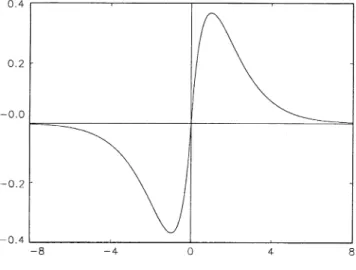
Fig. 1. IGFF(x) =xe−|x|.
instrument used for the lagged levelyi;t−1 is generated by the integrable IGF
F(yi;t−1) =yi;t−1e−ci|yi; t−1|;
where the factorci is inversely proportional to the sample standard error of Oyit=uit
andTi1=2. That is,
ci=KTi−1=2s−1(Oyit) withs2(Oyit) =Ti−1 Ti
t=1
(Oyit)2;
where K is a constant. The value of K is 2xed at 3 for all i= 1; : : : ; N, and for all combinations ofN andT considered here.7 We note that the factor c
i in the de2nition
of the instrument generating functionF is data-dependent through the sample standard error of the di)erence of the data yit. Hence, the value of ci will be determined for
each cross-sectional uniti=1; : : : ; N. The shape of the integrable IV generating function
F is given in Fig. 1.
Our asymptotics requires the factor ci to be constant. For practical applications,
however, we found it desirable to make ci dependent upon Ti as suggested in the
previous equation. With the choice of larger (smaller) value ofci, we may have better
size (power) at the cost of power (size). This is well expected. Notice that the larger the value of ci, the more integrable the IGF F becomes. Our asymptotics thus better
predicts 2nite sample behavior of the test. On the other hand, the test loses 2nite sample powers as the factor ci gets larger. As is well known from the standard regression
7The test SN constructed from the IGF F with a lager value of K tends to have smaller rejection
probabilities uniformly over all the choices ofN andT. The IGF de2ned withK= 3 seems to work best overally, and thus chosen for our simulations. For the cases where the time dimension is smallT= 25, the average nonlinear IV testSN slightly over-rejects the null. In such cases, one might use a little larger value ofK to correct the upward size distortion.
theory, the optimal IGF is given by the identityF(x) =x, which reduces our nonlinear IV estimator to the OLS estimator. As the IGF F tends to be more integrable, the resulting nonlinear IV estimator becomes less eHcient, which may lead to the power loss in our test.
To test the unit root hypothesis, we set i= 1 for all i= 1; : : : ; N, and
investi-gate the 2nite sample sizes in relation to the corresponding nominal test sizes. To examine the rejection probabilities under the alternative, we generate i’s randomly
from Uniform[0.8,1]. The model is thus heterogeneous under the alternative. The 2nite sample performance of the average nonlinear IV t-ratio statistic SN is
com-pared with that of the t-bar statistic by Im et al. (1997), which is based on the average of the individual t-tests computed from the sample ADF regressions (7) with mean and variance modi2cations. More explicitly, the t-bar statistic is de2ned as t-bar = √ N(RtN −N−1 iN=1 E(ti)) N−1N i=1 var(ti) ;
whereti is thet-statistic for testing i= 1 for the ith sample ADF regression (7), and
R
tN =N−1 Ni=1 ti. The values of the expectation and variance, E(ti) and var(ti), for
each individual ti depend on Ti and the lag-order pi, and computed via simulations
from independent normal samples. The number of time series observationTi for each
i= 1; : : : ; N is required to be the same.8
The panels with the cross-sectional dimensions N = 5;15;25;50;100 and the time series dimensionsT= 25;50;100 are considered for the 1%, 5% and 10% size tests.9 Since we are using randomly drawn parameter values, we simulate 20 times and re-port the ranges of the 2nite sample performances of the average nonlinear IV t-ratio statistic SN and the t-bar test. Each simulation run is carried out with 10,000
simu-lation iterations. Tables 1, 2 and 3 report, respectively, the 2nite sample sizes, the 2nite sample rejection probabilities and the size adjusted 2nite sample powers of the two tests. For each statistic, we report the minimum, mean, median and max-imum of the rejection probabilities under the null and the alternative hypotheses.
As can be seen from Table 1, the 2nite sample sizes of the test SN are quite close
to the corresponding nominal sizes. The sizes are calculated using the critical values from the standard normal distribution, and therefore the simulation results corroborate the asymptotic normal theory for SN. The limit theory seems to provide reasonably
good approximations even when the number of time series observation is relatively small, i.e., when T = 25, for all of the cross-sectional dimensions considered. On the other hand, the t-bar statistic exhibits noticeable size distortions, as reported, for
8Table 2 in Im et al. (1997) tabulates the values of E(ti) and var(ti) for T =
5;10;15;20;25;30;40;50;60;70;100 and forpi= 0; : : : ;8.
9For simplicity we use the sameT for all cross-sectional units in our simulations. However, our theory
does permit heterogeneity in the numberTi of time series observations. It is also true that thet-bar test can be practically implemented for unbalanced panels, though Im et al. (1997) do not explicitly allow for heterogeneousTi’s in their theoretical developments.
Table 1
Finite sample sizes
N T Tests 1% Test 5% Test 10% Test
Min Mean Med Max Min Mean Med Max Min Mean Med Max 5 25 t-bar 0.024 0.027 0.026 0.030 0.090 0.095 0.094 0.100 0.156 0.166 0.166 0.173 SN 0.018 0.021 0.021 0.024 0.065 0.071 0.071 0.075 0.117 0.124 0.124 0.130 15 25 t-bar 0.037 0.041 0.041 0.045 0.129 0.136 0.135 0.144 0.217 0.225 0.226 0.230 SN 0.017 0.020 0.020 0.022 0.063 0.071 0.071 0.076 0.114 0.124 0.124 0.131 25 25 t-bar 0.044 0.049 0.049 0.053 0.153 0.162 0.163 0.169 0.258 0.265 0.266 0.271 SN 0.015 0.017 0.018 0.020 0.057 0.066 0.067 0.071 0.108 0.118 0.118 0.125 50 25 t-bar 0.077 0.081 0.082 0.086 0.225 0.232 0.232 0.238 0.346 0.353 0.353 0.360 SN 0.015 0.017 0.017 0.019 0.058 0.063 0.063 0.068 0.106 0.115 0.115 0.121 100 25 t-bar 0.146 0.154 0.154 0.159 0.349 0.358 0.358 0.364 0.486 0.494 0.494 0.505 SN 0.015 0.017 0.018 0.019 0.058 0.063 0.064 0.066 0.109 0.114 0.115 0.118 5 50 t-bar 0.016 0.019 0.018 0.021 0.071 0.075 0.076 0.077 0.132 0.138 0.138 0.142 SN 0.016 0.018 0.018 0.021 0.059 0.065 0.066 0.072 0.109 0.116 0.116 0.123 15 50 t-bar 0.020 0.024 0.024 0.029 0.086 0.092 0.091 0.100 0.156 0.163 0.163 0.172 SN 0.014 0.016 0.017 0.017 0.059 0.062 0.062 0.065 0.104 0.111 0.111 0.120 25 50 t-bar 0.024 0.026 0.026 0.028 0.095 0.101 0.101 0.103 0.168 0.177 0.177 0.181 SN 0.010 0.014 0.014 0.016 0.050 0.055 0.056 0.060 0.096 0.102 0.101 0.109 50 50 t-bar 0.030 0.034 0.034 0.039 0.115 0.123 0.122 0.132 0.197 0.209 0.209 0.218 SN 0.010 0.012 0.012 0.013 0.045 0.050 0.050 0.053 0.087 0.093 0.094 0.098 100 50 t-bar 0.049 0.053 0.053 0.059 0.162 0.167 0.167 0.174 0.260 0.267 0.267 0.277 SN 0.009 0.011 0.011 0.014 0.040 0.045 0.045 0.048 0.079 0.085 0.085 0.089 5 100 t-bar 0.014 0.016 0.016 0.018 0.062 0.066 0.067 0.071 0.120 0.124 0.125 0.129 SN 0.014 0.017 0.017 0.019 0.060 0.063 0.064 0.068 0.109 0.115 0.115 0.120 15 100 t-bar 0.016 0.018 0.019 0.020 0.072 0.076 0.076 0.080 0.134 0.139 0.140 0.144 SN 0.013 0.015 0.015 0.017 0.052 0.059 0.059 0.063 0.100 0.107 0.107 0.112 25 100 t-bar 0.017 0.018 0.018 0.022 0.070 0.076 0.076 0.080 0.134 0.141 0.142 0.145 SN 0.011 0.013 0.013 0.015 0.049 0.052 0.052 0.056 0.091 0.098 0.098 0.102 50 100 t-bar 0.018 0.021 0.021 0.023 0.077 0.084 0.084 0.092 0.146 0.153 0.154 0.159 SN 0.010 0.011 0.011 0.013 0.042 0.046 0.047 0.050 0.083 0.087 0.087 0.092 100 100 t-bar 0.025 0.029 0.029 0.035 0.099 0.103 0.103 0.107 0.173 0.178 0.178 0.183 SN 0.007 0.010 0.009 0.012 0.038 0.041 0.040 0.045 0.073 0.078 0.078 0.084
instance, in the previous simulation work by Maddala and Wu (1999). The direc-tion of the size distordirec-tions are upward in all cases for all 1%, 5% and 10% tests. The t-bar statistic su)ers from severe size distortions especially when the number of cross-sectional units is large relative to the number of time series observations. For ex-ample, whenN= 100 and T= 25, the average 2nite sample sizes of the t-bar statistics for 1%, 5% and 10% tests are, respectively, 15%, 36% and 49%. The size distortions become less serious as the time dimension gets large; however, they are still quite noticeable.
The test SN is more powerful than the t-bar statistic for all 1%, 5% and 10%
tests and for all N and T combinations considered, as can be seen clearly from the results on the 2nite sample rejection probabilities and the size adjusted powers,
Table 2
Finite sample rejection probabilities
N T Tests 1% Test 5% Test 10% Test
Min Mean Med Max Min Mean Med Max Min Mean Med Max 5 25 t-bar 0.059 0.094 0.088 0.139 0.191 0.258 0.248 0.346 0.306 0.390 0.377 0.498 SN 0.073 0.132 0.119 0.225 0.207 0.316 0.297 0.465 0.319 0.445 0.428 0.607 15 25 t-bar 0.184 0.277 0.278 0.368 0.417 0.540 0.546 0.652 0.568 0.684 0.691 0.778 SN 0.223 0.364 0.364 0.526 0.449 0.617 0.625 0.767 0.590 0.741 0.750 0.862 25 25 t-bar 0.346 0.472 0.464 0.628 0.627 0.736 0.732 0.854 0.761 0.844 0.841 0.926 SN 0.397 0.577 0.575 0.780 0.655 0.804 0.808 0.928 0.778 0.887 0.892 0.968 50 25 t-bar 0.725 0.831 0.847 0.908 0.901 0.951 0.962 0.980 0.951 0.979 0.983 0.993 SN 0.780 0.901 0.917 0.969 0.930 0.975 0.980 0.995 0.965 0.990 0.992 0.998 100 25 t-bar 0.972 0.988 0.989 0.994 0.996 0.998 0.999 0.999 0.999 1.000 1.000 1.000 SN 0.987 0.996 0.997 0.999 0.998 1.000 1.000 1.000 0.999 1.000 1.000 1.000 5 50 t-bar 0.081 0.194 0.163 0.372 0.246 0.438 0.404 0.672 0.385 0.591 0.563 0.809 SN 0.189 0.382 0.337 0.651 0.417 0.642 0.614 0.877 0.566 0.765 0.752 0.943 15 50 t-bar 0.341 0.601 0.611 0.817 0.626 0.834 0.849 0.953 0.760 0.911 0.925 0.980 SN 0.648 0.861 0.879 0.979 0.867 0.959 0.971 0.998 0.929 0.982 0.990 1.000 25 50 t-bar 0.675 0.854 0.855 0.979 0.887 0.962 0.967 0.997 0.945 0.985 0.988 0.999 SN 0.912 0.981 0.988 1.000 0.984 0.997 0.999 1.000 0.994 0.999 1.000 1.000 50 50 t-bar 0.979 0.996 0.998 1.000 0.998 1.000 1.000 1.000 0.999 1.000 1.000 1.000 SN 1.000 1.000 1.000 1.000 1.000 1.000 1.000 1.000 1.000 1.000 1.000 1.000 100 50 t-bar 1.000 1.000 1.000 1.000 1.000 1.000 1.000 1.000 1.000 1.000 1.000 1.000 SN 1.000 1.000 1.000 1.000 1.000 1.000 1.000 1.000 1.000 1.000 1.000 1.000 5 100 t-bar 0.215 0.609 0.558 0.955 0.498 0.828 0.833 0.996 0.668 0.906 0.921 0.999 SN 0.530 0.830 0.843 0.998 0.791 0.946 0.964 1.000 0.883 0.975 0.987 1.000 15 100 t-bar 0.870 0.981 0.995 1.000 0.975 0.997 1.000 1.000 0.991 0.999 1.000 1.000 SN 0.996 1.000 1.000 1.000 1.000 1.000 1.000 1.000 1.000 1.000 1.000 1.000 25 100 t-bar 1.000 1.000 1.000 1.000 1.000 1.000 1.000 1.000 1.000 1.000 1.000 1.000 SN 1.000 1.000 1.000 1.000 1.000 1.000 1.000 1.000 1.000 1.000 1.000 1.000 50 100 t-bar 1.000 1.000 1.000 1.000 1.000 1.000 1.000 1.000 1.000 1.000 1.000 1.000 SN 1.000 1.000 1.000 1.000 1.000 1.000 1.000 1.000 1.000 1.000 1.000 1.000 100 100 t-bar 1.000 1.000 1.000 1.000 1.000 1.000 1.000 1.000 1.000 1.000 1.000 1.000 SN 1.000 1.000 1.000 1.000 1.000 1.000 1.000 1.000 1.000 1.000 1.000 1.000
reported, respectively, in Tables 2 and 3. The discriminatory power of SN is
notice-ably much higher than that of the t-bar statistic for the cases with smaller T and
N. For the 1% tests with the combinations (N; T) ={(15;25);(25;25);(5;50)}, the power of the testSN is more than twice as large as that of thet-bar statistic. The SN
still performs much better than the t-bar even when T is large, if the cross-sectional dimension is small. The performance of the t-bar statistic improves as both N and
T increase, though the improvement is more noticeable with the growth in T. The di)erences in the 2nite sample powers of SN and t-bar vanish as both N and T
Table 3
Finite sample powers
N T Tests 1% Test 5% Test 10% Test
Min Mean Med Max Min Mean Med Max Min Mean Med Max 5 25 t-bar 0.022 0.041 0.040 0.068 0.109 0.156 0.149 0.217 0.201 0.269 0.260 0.349 SN 0.034 0.077 0.069 0.143 0.157 0.250 0.236 0.393 0.271 0.392 0.379 0.554 15 25 t-bar 0.062 0.110 0.108 0.165 0.208 0.310 0.305 0.398 0.340 0.462 0.456 0.567 SN 0.150 0.257 0.245 0.390 0.367 0.540 0.543 0.692 0.529 0.693 0.695 0.827 25 25 t-bar 0.138 0.208 0.196 0.336 0.342 0.473 0.462 0.627 0.486 0.625 0.619 0.759 SN 0.344 0.484 0.464 0.714 0.607 0.761 0.760 0.901 0.748 0.866 0.867 0.957 50 25 t-bar 0.354 0.482 0.501 0.584 0.627 0.753 0.772 0.854 0.761 0.860 0.869 0.927 SN 0.707 0.858 0.879 0.944 0.911 0.966 0.973 0.993 0.958 0.987 0.990 0.998 100 25 t-bar 0.713 0.806 0.806 0.868 0.895 0.944 0.946 0.966 0.950 0.976 0.978 0.987 SN 0.980 0.993 0.994 0.998 0.997 1.000 1.000 1.000 0.999 1.000 1.000 1.000 5 50 t-bar 0.047 0.129 0.111 0.280 0.176 0.352 0.320 0.584 0.306 0.507 0.479 0.730 SN 0.128 0.293 0.251 0.537 0.353 0.586 0.548 0.845 0.526 0.733 0.713 0.926 15 50 t-bar 0.192 0.451 0.483 0.687 0.480 0.734 0.752 0.898 0.640 0.847 0.859 0.959 SN 0.569 0.813 0.826 0.963 0.842 0.949 0.958 0.996 0.922 0.979 0.986 1.000 25 50 t-bar 0.496 0.735 0.732 0.943 0.783 0.915 0.921 0.991 0.884 0.962 0.967 0.997 SN 0.891 0.974 0.984 1.000 0.978 0.997 0.999 1.000 0.994 0.999 1.000 1.000 50 50 t-bar 0.919 0.980 0.990 0.999 0.987 0.998 0.999 1.000 0.997 0.999 1.000 1.000 SN 1.000 1.000 1.000 1.000 1.000 1.000 1.000 1.000 1.000 1.000 1.000 1.000 100 50 t-bar 0.999 1.000 1.000 1.000 1.000 1.000 1.000 1.000 1.000 1.000 1.000 1.000 SN 1.000 1.000 1.000 1.000 1.000 1.000 1.000 1.000 1.000 1.000 1.000 1.000 5 100 t-bar 0.182 0.540 0.480 0.925 0.441 0.786 0.785 0.993 0.615 0.882 0.899 0.999 SN 0.432 0.774 0.771 0.993 0.753 0.929 0.950 1.000 0.864 0.970 0.984 1.000 15 100 t-bar 0.777 0.966 0.988 1.000 0.950 0.994 1.000 1.000 0.982 0.998 1.000 1.000 SN 0.986 0.998 1.000 1.000 0.999 1.000 1.000 1.000 1.000 1.000 1.000 1.000 25 100 t-bar 0.992 0.999 1.000 1.000 1.000 1.000 1.000 1.000 1.000 1.000 1.000 1.000 SN 1.000 1.000 1.000 1.000 1.000 1.000 1.000 1.000 1.000 1.000 1.000 1.000 50 100 t-bar 1.000 1.000 1.000 1.000 1.000 1.000 1.000 1.000 1.000 1.000 1.000 1.000 SN 1.000 1.000 1.000 1.000 1.000 1.000 1.000 1.000 1.000 1.000 1.000 1.000 100 100 t-bar 1.000 1.000 1.000 1.000 1.000 1.000 1.000 1.000 1.000 1.000 1.000 1.000 SN 1.000 1.000 1.000 1.000 1.000 1.000 1.000 1.000 1.000 1.000 1.000 1.000 7. Empirical illustrations
In this section, we apply the newly developed panel unit root testSN to test whether
the PPP hypothesis holds. The PPP hypothesis has been tested by many researchers using various unit root tests, both in panel as well as in univariate models. Exam-ples include MacDonald (1996), Frankel and Rose (1996), Oh (1996), Papell (1997), O’Connell (1998), just to name a few. There have been, however, conSicting evidence, and the issue does not seem to be completely settled.
We consider the data used in Papell (1997), which consists of the real exchange rates for 20 countries computed from the IMF’s International Financial Statistics (IFS)
Table 4
PPP tests for IFS data
t-bar SN T= 50 T= 100 T= 50 T= 100 AR 2 −1:589b −1:183 −2:872a −2:554a Order 4 −7:108a −4:525a −5:969a −5:119a BIC 4 −2:740a −3:490a −3:719a −4:695a Max order 8 −1:127 −2:646a −0:249 −3:937a
Note: The superscripts a, b and c denote, respectively, the statistical signi2cance at 1%, 5% and 10% levels.
tape, covering the period 1973:1–1998:4.10 We also consider the data from the Penn World Table (PWT) analyzed in Oh (1996).11 The empirical results are summarized in Tables 4 and 5, respectively, for the results obtained from the data from Papell (1997) and Oh (1996). We allow the models to have heterogeneous dynamic structures, i.e., the models may have di)erent AR orders for individual cross-sectional units. For each cross-sectional unit the AR order is selected using the BIC criterion with the maximum number of lags 4 or 8 for the quarterly IFS data, and with 2 or 4 for the annual PWT data. To see how sensitive are the test results with respect to the speci2cations of individual dynamics, we also look at the panels with homogeneous dynamics, where we do not allow the AR order to vary across the individual units and 2x the AR order for all cross-sectional units at 2 or 4 for the IFS data and at 1 or 2 for the PWT data. For the analysis of the PWT data, we looked at four di)erent groups of countries. For each groupof countries, the numbers of the time series observations are di)erent, varying from 30 to 41.12 The IFS data have total 104 time series observations. To examine the dependency on the sample size also for the test results from the IFS data set, we considered two sub-samples of sizes 50 and 100. The sub-samples are obtained by retaining the most recent observations.
For both data from Papell (1997) and Oh (1996), our test strongly rejects the unit root hypothesis, which is used in the empirical studies as an indirect evidence for the PPP relationship. As seen from Tables 4 and 5, our test rejects the presence of the
10The quarterly data used in Papell (1997) covers the period 1973:1–1994:3, but the data used here is
extended to 1998:4. The countries considered include Austria, Belgium, Denmark, Finland, France, Germany, Italy, Japan, Netherlands, Norway, Spain, Sweden, Switzerland, United Kingdom, Ireland, Australia, Greece, New Zealand, Portugal, and Canada. The real exchange raterit for theith country is computed using the US dollar as the numeraire currency, and calculated asrit= log(eitp∗t=pit), whereeit; p∗t andpit denote,
respectively, the nominal spot exchange rate for theith country, the US CPI, and the CPI for theith country.
11The data used in Oh (1996) are yearly observations from the Penn World Table, Mark 5.5. The data
are collected for 111 countries for the period 1960–1989, and extended to a longer period 1950–1990 for a group of 51 countries. For the longer sample, the data are analyzed for two sub-samples, the 22 OECD countries and G6 countries (Canada, France, Germany, Italy, Japan and United Kingdom).
12For the groupof 111 countries, there are 30 annual observations. But for the groupof 51 countries
Table 5
PPP tests for PWT data
t-bar SN
G6 OECD 51Con 111Con G6 OECD 51Con 111Con
AR 1 −1:014 −1:997b −2:694a −6:111a −1:471c −3:217a −4:116a −8:066a
Order 2 −0:400 −0:669 −0:912 −3:420a −0:629 −1:528c −1:975b −5:033a
BIC 2 −1:014 −1:997b −2:066b −4:279a −1:471c −3:217a −3:841a −6:708a
Max order 4 −1:014 −1:723b −2:062b −3:899a −1:471c −3:103a −3:740a −6:002a
Note: The superscripts a, b and c denote, respectively, the statistical signi2cance at 1%, 5% and 10% levels.
unit root in most of the cases considered here.13 The values of the test statistic S
N
of course vary for di)erent choices of the sample size T and the speci2cations of the dynamic structures, but overall they provide strong evidence against the null hypothesis of the unit root. Our test appears to be fairly robust with respect to the speci2cations of model dynamics and the sizes of the samples.
In sharpcontrast, the t-bar test by Im et al. (1997) produces the results that are inconclusive. The test results are, in particular, quite sensitive to the speci2cations of the individual dynamic structures, and to the dimensions of the cross-sectional and time series observations. For the IFS data, we get contradictory results for each choice of the number of time series observations and maximum order in the BIC criterion. It appears that the test has the tendency to support the PPP when the sample size is large. However, this tendency is not observed when we do not allow for hetero-geneous dynamics across individual units. The results from the PWT data are also inconclusive. Thet-bar test supports or rejects the PPP depending upon how we select the countries and the time series observations. The test fails to consistently reject the presence of the unit root except for one case where we have largest number of total observations.
8. Conclusions
This paper introduces an asymptotically normal unit root test for panels with cross-sectional dependency. The test is based on nonlinear IV estimation of the autoregressive coeHcient using the instruments generated by the class of regularly integrable func-tions. Thet-ratio statistic for the test of the unit root constructed from such nonlinear
13Our test is not able to reject the absence of PPP for 20 OECD countries from the IFS data when
short-run dynamics is selected by the BIC with the larger maximum number of lags 8 and the smaller time dimensionT= 50. This might be due to the fact that the 50 quarterly time series observations (possibly with upto 8 losses in data points for constructing lagged di)erences) amount to only about 12 years of time span, which is too short for uncovering long-run properties of the underlying stochastic processes. Our test also fails to reject the null for G6 countries based on the PWT data, when the dynamics is restricted at AR(2). This indeed is the case with the smallest number of total observations, which may well have led to the low power.
IV estimator is shown to have standard normal limit distribution, for each individual cross-sectional uniti=1; : : : ; N. The nonlinear IV t-ratio statistic has simple symmetric con2dence intervals both under the unit root null as well as under the stationarity alter-natives. Therefore, there are no more discontinuity problems in the con2dence intervals in the transition from stationary to nonstationary cases. The same results extend to the models with deterministic trends. More importantly, we show that the limit distribu-tions of the nonlinear IV t-ratio statistics for testing for the unit root in individual cross-sectional units are cross-sectionally independent.
The asymptotic orthogonalities among the individual nonlinear IV t-ratio statis-tics naturally lead us to propose a standardized sum of the individual IV t-ratios for the test of the unit root for panels with cross-sectional dependency. We show that the limit theory of such standardized sum of individual nonlinear IV t-ratios, which we call the SN statistic, is also standard normal. The limit theory is derived
via T-asymptotics, which is not followed by N-asymptotics. The spatial dimension consequently is not required to be large, and therefore it may take any value, large or small. Moreover, the number of time series observations is allowed to be dif-ferent across cross-sectional units, and thus our panel nonlinear IV method permits unbalanced panels. This implies that we can do simple inference based on the stan-dard normal distribution even for unbalanced panels with general cross-sectional dependency.
The simulation results seem to well support our theoretical 2ndings. The 2nite sam-ple sizes ofSN calculated from using the standard normal critical values quite closely
approximate the nominal test sizes. Moreover, the test SN has noticeably higher
dis-criminatory power than the commonly used average panel unit root test t-bar by Im et al. (1997). The panel nonlinear IV unit root test seems to improve signi2cantly upon the t-bar test under cross-sectional dependency, especially for the panels with smaller time and spatial dimensions. The new statistic SN is applied to test whether
the PPP hypothesis holds, using the data sets from the International Financial Statis-tics and the Penn World Table. Our test appears to be fairly robust to the speci2-cations of the model dynamics and the sizes of the samples, and strongly supports the PPP relationship, while the t-bar test by Im et al. (1997) produces inconclusive results.
Acknowledgements
I thank the Co-Editors and two anonymous referees for many constructive com-ments and suggestions. The paper was prepared for the presentation at the Cardi) Conference on Long Memory and Nonlinear Time Series, and completed while I was visiting the Center for the International Research on the Japanese Economy (CIRJE), University of Tokyo. I am very grateful to Fumio Hayashi, Naoto Kunitomo and Yoshi-hiro Yajima for their hospitality and support. My thanks also go to David Papell and Keun-Yeob Oh for kindly providing the data sets used here for empirical illustra-tions, and to Paul Evans, Joon Park and Peter Phillips for helpful discussions and comments.
Appendix: Mathematical proofs
Proof of Lemma 3.2. We have from the Beveridge–Nelson representation ofyit given
in (6) that Ti−1=2yi[Tir]=i(1)Ti−1=2 [Tir] t=1 it+ op(1);
wherei(1) =i(1)−1. Then we have as Ti→ ∞
Ti−1=2yi[Tir]=i(1)UiTi(r) + op(1)→d i(1)Ui(r); (A.1) since UiTi →d Ui as Ti → ∞; due to the invariance principle in (4). Then it follows from Lemma 5 (c) of Chang et al. (2001) that
Ti−1=4Ti t=1 F(yi;t−1)it→d#i Li(1;0) ∞ −∞F(i(1)s) 2ds 1=2 Wi(1) = #i i(1)L i(1;0) ∞ −∞F(s) 2ds1=2W i(1)
by a simple change of variables. This establishes the result in part (a).
The stated result in part (b) is obtained similarly using the result in Lemma 5 (i) of Chang et al. (2001) as follows:
Ti−1=2 Ti t=1 F(yi;t−1)2→dLi(1;0) ∞ −∞F(i(1)s) 2ds = i(1)L i(1;0) ∞ −∞F(s) 2ds
again by a simple change of variables.
For part (c), just note that Oyi;t−1; : : : ;Oyi;t−pi are stationary regressors, and then
the proof follows directly from the asymptotic orthogonality between the integrable transformations of integrated processes and stationary regressors established in part (e) of Lemma 5 in Chang et al. (2001).
Proof of Theorem 3.3. We begin by investigating the limit behavior of ATi and CTi de2ned below (11). Recall x
it= (Oyi;t−1; : : : ;Oyi;t−pi). Then it follows from Lemma 3.2 (c) that
Ti
t=1
which gives Ti t=1 F(yi;t−1)xit T i t=1 xitxit −1Ti t=1 xitit 6 Ti t=1 F(yi;t−1)xit T i t=1 xitxit −1 Ti t=1 xitit =op(Ti3=4)Op(Ti−1)Op(Ti1=2) =op(Ti1=4) and Ti t=1 F(yi;t−1)xit T i t=1 xitxit −1Ti t=1 xitF(yi;t−1) 6 Ti t=1 F(yi;t−1)xit T i t=1 xitxit −1 Ti t=1 xitF(yi;t−1) =op(Ti3=4)Op(Ti−1)op(Ti3=4) =op(Ti1=2): Then we have Ti−1=4ATi=Ti−1=4 Ti t=1 F(yi;t−1)it+ op(1) and Ti−1=2CTi=Ti−1=2 Ti t=1 F(yi;t−1)2+ op(1):
Next we write Zi de2ned in (12) as
Zi=ˆsi( ˆ− 1 i) = BT−i1ATi ( ˆ#2 iB−Ti2CTi)1=2 = ATi ˆ #iCT1=i2
using the results in (11) and (13). Then it follows immediately from Lemma 3.2 (a) and (b) that Zi = T −1=4 i ATi ˆ #i(Ti−1=2CTi)1=2 = Ti−1=4 Ti t=1 F(yi;t−1)it ˆ #i(Ti−1=2tT=1i F(yi;t−1)2)1=2 + op(1)