Simplifying Encoder-Decoder-Based Neural Machine Translation Systems to Translate between Related Languages

(1)

Trabajo Fin de Grado

Autor:

Lucas Gil Melby Tutor/es:

Juan Antonio Pérez Ortiz 

Felipe Sánchez Martínez

Septiembre 2018

Simplifying

Encoder-Decoder-Based

Neural Machine Translation

Systems to Translate between

Related Languages

(2)

Universidad de Alicante

Escuela Polit´ecnica Superior

Departamento de Lenguajes y Sistemas Inform´

aticos

Simplifying Encoder-Decoder-Based Neural

Machine Translation Systems to Translate

between Related Languages

Lucas Gil Melby

Submitted in part fulfilment of the requirements for the degree of

(3)

Abstract

Neural machine translation is one of the most advanced approaches to machine translation and one that is recently obtaining good enough results to make use of it in real-life scenarios. The currently widely used architecture is what is known as sequence-to-sequence architecture with attention mechanism, which uses an encoder to create a vector representation of the input sentence in source language, a decoder to output a sentence in target language and an attention mechanism to help the decoder produce more accurate outputs.

The simplification of state-of-the-art sequence-to-sequence neural machine translation with at-tention is explored in this work for the translation between related languages. First, some of the state-of-the-art features present in the baseline system are presented and described. The main hypothesis of this work is the possibility of removing these features without worsening the translation quality too much and simplifying the network’s structure at the same time when translating between related languages. The main part of this work is the substitution of state-of-the-art attention mechanisms, used to help the decoder know which part of the source sentence is more relevant for the part of the target sentence being outputted, by a simplified attention mechanism which mostly pays attention to the word in the source sentence in the same position as the current target word.

The simplification is carried out by removing beam search (a technique used to explore a wider range of possible outputs instead of limiting the output to the highest probability of being the correct output), substituting the bidirectional encoder by a unidirectional encoder and creating a new “local attention” mechanism in replacement for the current more complex state-of-the-art attention mechanism.

Once the simplifications have been discussed and implemented, their impact on translation quality for related languages (Spanish and Catalan in the case of this work) is tested and compared to determine their suitability. From the results obtained, as expected, the removal of beam search and the substitution of the bidirectional encoder by a unidirectional encoder does not have a great impact on translation quality, resulting in a decrease of 6%-23% in BLEU score depending on the attention mechanism being used.

On top of this, the introduction of the newly-developed “local attention” mechanism improves translation quality by 176% and 218% in BLEU score when compared to an attention-less

(4)

system, about 22%-27% less than the state-of-the-art attention mechanism used in the baseline system.

All of this resulting in the great simplification in the network, reducing the number of trainable parameters from 12.195.945 to 9.816.485 (19.5%) and the training time from 22h 53m to 12h 15m.

(5)

Acknowledgements

I would like to express my sincere gratitude to:

My supervisors Juan Antonio P´erez Ortiz and Felipe S´anchez Mart´ınez.

The whole Transducens research group because they have made me feel welcome in their group and have awakened my curiosity for the scientific perspective of computer science.

My friend Mart´ın who has helped me a lot throughout this journey.

(6)

(7)

List of Tables

5.1 Corpora sizes in sentences . . . 27

6.1 Evaluation Results in BLEU . . . 32

(12)

(13)

List of Figures

2.1 LSTM Unit . . . 5

2.2 GRU Unit . . . 5

2.3 Vectors Connecting Similar Word Embeddings . . . 6

2.4 Unidirectional Encoder . . . 7

2.5 Bidirectional Encoder . . . 8

2.6 Decoder . . . 9

2.7 Beam Search Probabilities . . . 10

2.8 Attention Mechanism . . . 12

2.9 Attention Vector . . . 13

4.1 English to Spanish Attention Matrix . . . 19

4.2 Catalan to Spanish Attention Matrix . . . 20

4.3 Spanish to Catalan translation . . . 21

4.4 Attention vectors with gaussian distribution . . . 22

4.5 Different bell width Gaussian attention vectors . . . 26

5.1 Different attention vectors . . . 29 xi

(14)

5.2 Translation qualities with Gaussian attention with different bell widths . . . 30 5.3 Gaussian attention vector with bell width of 0.3 . . . 30

(15)

Chapter 1 Introduction

Communication among speakers of different languages has always been a challenge since the emergence of the first human languages. In recent years, manual translation of contents has been strengthened by machine translation techniques.

The development of new machine translation systems has advanced a lot since the creation of the first machine translation system [Reynolds, A. Craig, 1954]. Although they first appeared in 1997 [ ˜Neco and Forcada, 1997] with some precursors in the early 90s [Chalmers, 1990, Chrisman, 1991], in the last few years, since the appearance of the first production-ready neural machine translation (NMT) systems in 2013 [Kalchbrenner and Blunsom, 2013, Sutskever, Vinyals and Le, 2014], the popularization of neural machine translation, thanks partly to the development and availability of GPUs, has enabled much quicker and more extensive network training.

Neural networks applied to machine translation, with its limitations such as the need of very large parallel corpora (although some authors have proposed methods to overcome this lim-itation [Artetxe et al., 2017]) or its sensitiveness to low quality corpora, have shown very promising results in machine translation, specifically when large, high quality bilingual corpora are available.

Due to their nature, many neural machine translation systems such as those based on the sequence-to-sequence architecture [Bahdanau et al., 2014] with attention which are covered

(16)

2 Chapter 1. Introduction

in this work, are prone to errors under certain circumstances such as the translation of long sentences, sentences with rare or uncommon words or the translation of sentences between distant languages, more noticeable when word order changes a lot from one language to the other [Koehn and Knowles, 2017].

To cope with each of these and other problems, many techniques have been developed and ap-plied on top of the widely used basic sequence-to-sequence architecture (also known as encoder-decoder), hence creating very complex and fine tuned NMT systems. One example could be TensorFlow’snmt project [Luong et al., 2016], which gathers a whole collection of existing tech-niques such as bidirectional encoders, beam search, LSTM and GRU units, byte pair encoding [Witten et al., 1994], and new features like Luong’s attention mechanism [Luong et al., 2016], etc.

However, some of these innovations are aimed at improving translations in complex situations and for challenging language pairs but the hypothesis explored in this work is that these innova-tion may not contribute too much to the translainnova-tion quality in certain situainnova-tions such as related languages translations. The work here described focuses on either removing or modifying some of these features in order to create a simplified version of the encoder-decoder architecture for NMT to deal with related language pairs reducing the number of trainable parameters, training and translation time while keeping a decent translation quality.

(17)

Chapter 2 Encoder-Decoder Recurrent

Architecture for NMT

2.1 Encoder-Decoder NMT Overview

The basic encoder-decoder architecture [Sutskever et al., 2014] is based on the idea of producing some sort of internal representation of the sentence to be translated before any output is produced; this is the work of the encoder, which based on the sequential input of source words and an internal state ends up creating a vector representation of the input sentence.

The second part of the basic idea behind encoder-decoder architectures is the use of this sentence representation to produce an output. This is the responsibility of the decoder, which also sequentially and based on the vector representation produced by the encoder, its own internal state and the previously outputted word produces the next target word.

To cope with some of the most common challenges in neural machine translation, NMT has ben-efited from many innovative solutions previously developed and has introduced others. Some of the most important are LSTM/GRU units to deal with the vanishing gradient issue [Hochre-iter., 1991, Hochreiter et al., 2001] (very useful when the context of long or very long sentences needs to be stored in the network’s cells for a an arbitrary time span), bidirectional encoder

(18)

4 Chapter 2. Encoder-Decoder Recurrent Architecture for NMT

(important to be able to take the whole input sentence into account when producing each tar-get word), attention mechanism (also useful for long and complex sentences), beam search (to mitigate the possible mistakes made by the network throughout the process of translation), etc. All of these ideas are introduced in this chapter.

2.2 LSTM and GRU Units

Since the introduction of Long Short-Term Memory (LSTM) units [Hochreiter, Schmidhuber, 1997], it has been possible to reduce the training deadlock caused by the vanishing gradient problem [Hochreiter., 1991, Hochreiter et al., 2001] in situations where gradient-based learning and backpropagation are used; training is obstructed and slowed down when long-term depen-dencies happen. LSTM units act as memory units which keep an internal state stored until it is needed. For example, in the context of NMT, LSTM units used in the encoder receive the context from the part of the sentence that has already been processed by the encoder (ht−1), the

representation of the current source word to process (xt) and combines these with its internal

state (ct−1) to produce a new internal state (ct) and a new encoder state (ht) with the new

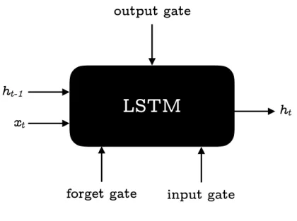
information coming from the added word and the LSTM unit’s internal state. To do so, as seen in Fig. 2.1 an LSTM unit uses three gates, the first one is the input gate, which controls what part and how much of the inputted sentence context (i. e. the part of the sentence previously processed by the encoder) and next-word-to-translate’s representation’s information is to be kept in the unit’s internal state. The second gate is the forget gate, which determines how much and what part of the unit’s internal state is to be forgotten before it is combined with the new inputted information. Finally, the output gate decides what part and how much of the newly updated internal state is going to be outputted as the new encoder context (ht).

(19)

2.2. LSTM and GRU Units 5 ht forget gate

LSTM

output gate input gate ht-1 xt Figure 2.1: LSTM Unit

The later introduction of Gated Recurrent Units (GRUs) [Cho et al., 2014], seen in Fig. 2.2, are a simplified version of LSTM units which combine the forget gate and the input gate into a single update gate, turned the use of gated units into a much more affordable option due to their computational simplicity [Chung et al., 2014].

update gate

GRU

ht-1 xt ht output gate

(20)

2.3 Word Embeddings

Natural language processing (NLP) networks need a way to work with the input they get, words in their string form are not an option as they cannot be used by networks. An approach to this issue is to map each word to a word embedding, a vector representation of words. These vectors are low dimensional vectors of continuous values. Thanks to this, this representation is much more efficient than a vector with as many dimensions as source vocabulary words.

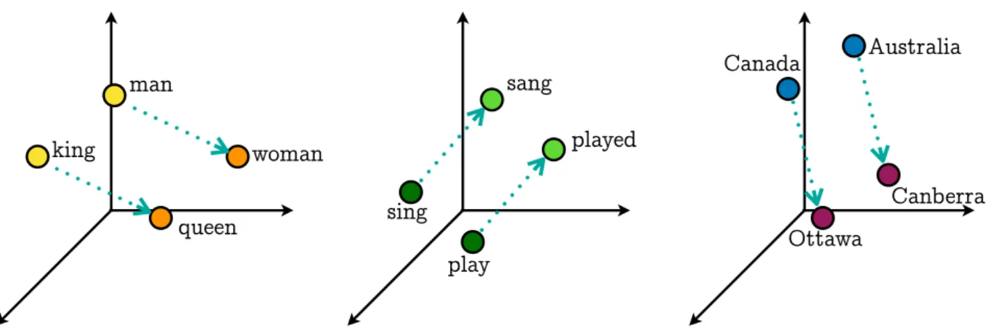
Another advantage of this approach is the contextual similarity of word embeddings, meaning that the position of each embedding in the n-dimensional space gives an overview of the word’s meaning, and their proximity to other embeddings show their similar meanings.

queen woman man king sang played sing play Canada Ottawa Canberra Australia

Figure 2.3: Vectors Connecting Similar Word Embeddings

This relation between position and meaning can even be extended to the point where arith-metic operations can be performed on embeddings showing different semantic properties. For example, the vector resulting from the subtraction of the embeddings of king and queen can be added to man to get something very similar towoman’s embedding. Likewise, the vectors connecting a verb and its past tense or a country and its capital city are also very similar.

(21)

2.4. Bidirectional Encoder 7

2.4 Bidirectional Encoder

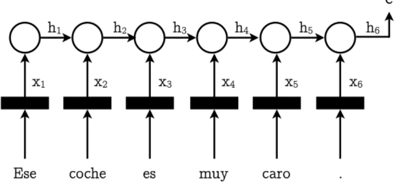
In an encoder-decoder architecture [Sutskever et al., 2014], the encoder, shown in Fig. 2.4, is in charge of creating a multidimensional vector representation c of the input sentence (which will later be used by the decoder to produce the target language representation). This vector representation is computed word by word, recomputing the context every time a new word xt

is used to produce a new encoder state ht.

Ese coche es muy caro .

h1 h2 h3 h4 h5 h6

x1 x2 x3 x4 x5 x6

c

Figure 2.4: Unidirectional Encoder

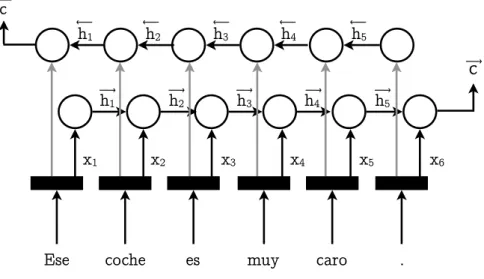
The method used to computecmakes long sentences difficult to represent, the way the meaning of each word (mapped as embeddings) is sequentially added to the preexisting context of the preceding part of the sentence ends up giving more importance to one end of the sentence rather than giving the same importance to the whole sentence. This creates a huge problem for long sentences, where one end of the sentence ends up being forgotten by the network, having a small influence on vector c. To try to solve this issue, bidirectional encoders like the one in Fig. 2.5 were introduced to make sure both the preceding and the following parts of the sentence have an influence on each encoder stated at each time-step and therefore on the final cvector.

(22)

Ese coche es muy caro .

h1 h2 h3 h4 h5 x1 x2 x3 x4 x5 x6

c

h1 h2 h3 h4 h5 c ⟶ ⟶ ⟶ ⟶ ⟶ ⟶ ⟶ ⟶ ⟶ ⟶ ⟶ ⟶

Figure 2.5: Bidirectional Encoder

Thanks to this introduction, two encoder state vectors (−→c for the forward state and ←−c for the backward state) are produced in inverse order. This way, the influence of the first part of the sentence in the forward state is compensated by the backward state and vice-versa.

The final context vectorcis usually obtained by simply concatenating the forward and backward context vectors.

An additional motivation for the introduction of bidirectional encoders is the possibility of including the context of both the previous and the future part of the sentence in each encoder state, which, as explained in Section 2.6, will later be used for the attention mechanism. This improvement to the unidirectional model has shown particularly good results in long sentences where taking both ends of the sentences into account helps to produce more realistic sentence representations.

2.5 Beam Search

The other component of the encoder-decoder architecture is the decoder. This component turns the context vector of a source sentence cinto a sentence in the target language. A decoder, as shown in Fig. 2.6, works using the context vectorc, which gives the decoder an overview of the

(23)

2.5. Beam Search 9

whole sentence meaning, the decoder’s previous state st−1, a vector representation of what the

decoder has already processed, and finally the last outputted word yt−1, and then produces a

new decoder state st and the probability of each target vocabulary word of being the correct

translationyt(this probability is normalized with the normalized exponential function softmax

and then the maximum probability word is selected through one-hot encoding, a vector with as many positions as words in the (target) vocabulary, where all positions are set to 0 except for the selected word, which has a value of 1).

c

That car is very big .

s1 s2 s3 s4 s5 s6

s0

Figure 2.6: Decoder

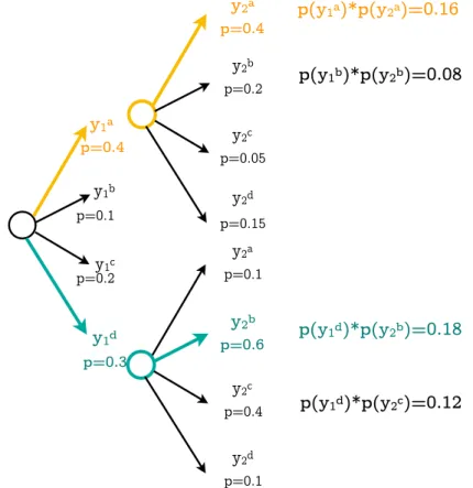
If the correct word that should be outputted is not the word with highest probability of being the correct option (p in Fig. 2.7) it will not only not be selected to be outputted, but an incorrect word will be re-fed into the decoder, which will affect the rest of the sentence negatively, making the decoder vulnerable to its own mistakes. Therefore, when using this technique, a simple mistake in one word could have a big effect on the whole sentence, this is why beam search was introduced in the decoder.

Beam search is a method used to try to avoid making mistakes while performing greedy decod-ing, by choosing not only the word with highest probability of being correct as the decoder’s output, but choosing more than one to explore other possible outputs. This way, a fixed num-ber of possible outputs are considered in each time-step dividing the translation into multiple parallel executions but keeping only the n translations with higher probabilities.

(24)

10 Chapter 2. Encoder-Decoder Recurrent Architecture for NMT p=0.3 p=0.4y 1a y1b y1c y1d p=0.1 p=0.2 p=0.4y 2a p=0.2 y2b p=0.05 y2c p=0.15 y2d p=0.1 y2a p=0.6y 2b p=0.4 y2c p=0.1 y2d p(y1a)*p(y2a)=0.16 p(y1b)*p(y2b)=0.08 p(y1d)*p(y2b)=0.18 p(y1d)*p(y2c)=0.12

Figure 2.7: Beam Search Probabilities

Thanks to this approach, as Fig. 2.7 shows, choosing the word with the second highest prob-ability ends up with a higher total probprob-ability for the two-word-sentence yd

1, y2b (0.3 x 0.6 =

0.18) than choosing the word with highest probability in each step (ya

1, y2a, 0.4 x 0.4 = 0.16).

In this case we have explored the two options with highest probability; this is known as a beam search with a beam of size 2.

Obviously all options cannot always be explored (which would be equivalent to a beam of size equal to the vocabulary), and therefore a sensible beam size has to be chosen taking computational power and time availability into account. To this date, most state of the art setups use a beam size of 5 [Freitag and Al-Onaizan, 2017, Huang et al., 2017].

(25)

2.6. Attention Mechanism 11

2.6 Attention Mechanism

The attention mechanism [Bahdanau et al., 2014] is one of the greatest improvements made to the encoder-decoder architecture until now and is very related to the nature of this architecture. The introduction of the attention mechanism aims at making the most out of the sentence context vector c. As already seen, traditional encoder-decoder architectures use the encoder to create a representation of the whole sentence (c) which is consumed later by the decoder, which produces the sentence in target language by looking at this representation (among other things).

This approach has its limitations, one of them is the decoder having to produce each target word based on a constant context vector which represents the whole sentence no matter which part is being translated at each time-step. To try to solve this problem, the attention mechanism was introduced.

The attention mechanism has a very concrete goal: to determine which part of the input to pay attention to in order to translate a particular target word. This is done by tweaking the context vector c so that the relevant input has a stronger influence in it. For this purpose, a specific context vector ci is computed to be used at each time-step i to produce each target

wordyi.

Bahdanau’s attention [Bahdanau et al., 2014] was the first one to be introduced and is still to this day, along with Luong’s modified version [Luong et al., 2016], the most popular choice for attention mechanisms.

For Bahdanau’s attention, this new tweaked context vector is produced by multiplying a weight-ing factorαij by the encoder state for each input word (let it be a simple unidirectional encoder

state, hi or the concatenation of the forward and backward state of a bidirectional encoder − → hi; ←− hi): ci = Tx X j=1 αijhj

(26)

Where αij indicates the influence of the input xj (through its correspondent encoder state hj)

of a sentence of length Tx to produce the target yi and is computed like this:

αij = elij PTx k=1elik , lij = a(si−1, hj)

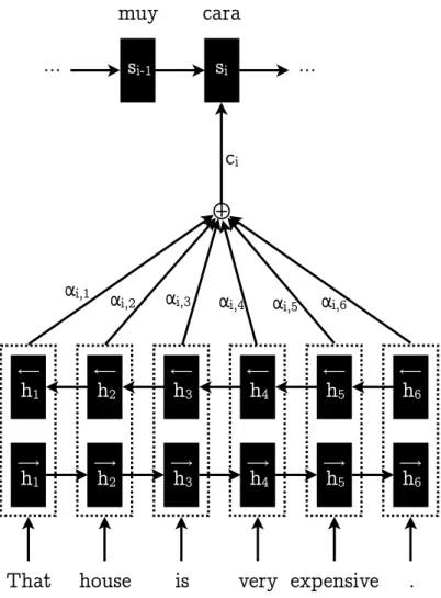
So as shown in Fig. 2.8, ci is now different for each decoder time-step, when the decoder is fed

with a weighted sentence context vector which gives more importance to input words relevant to the word being translated in that time-step.

h

1 ⟶

h

1 ⟶

That

h

2 ⟶

h

2 ⟶

house

h

3 ⟶

h

3 ⟶

is

h

4 ⟶

h

4 ⟶

very

h

5 ⟶

h

5 ⟶

expensive

h

6 ⟶

h

6 ⟶

.

⊕

s

i-1

s

i

muy

cara

...

α

i,1

_α

_i,2

_α

_i,3

_α

i,4

α

i,5

α

i,6

c

i

(27)

the house is

very exp

ensiv

e

.

Figure 2.9: Attention Vector

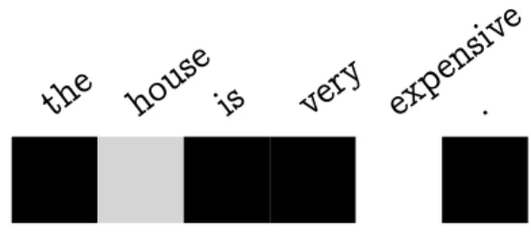
In this graphic representation of a vector containing all αi, the lighter the color the higher the

α factor is, and therefore, the more attention is payed to that input word.

As an example, a vector containing allαij for an outputyiwould look something similar to Fig.

2.9, where the attention mechanism is clearly telling the decoder to pay a lot of attention to the source word “expensive” when translating the word “cara”, which makes sense as “cara” is the translation of “expensive”. However, it is also worth noting that the attention mechanism is also telling the decoder to take “house” into account, and this is because when translating into Spanish, adjectives like “cara” have a number and a gender, and the only way of getting that information from an English sentence is from the noun, “house” in this case.

Thanks to the attention model, the network produces translations of a much greater quality as explained in Bahdanau’s [Bahdanau et al., 2014] and Luong’s [Luong et al., 2016] papers, specially for long sentences, as the decoder can focus on the specific relevant parts of a sentence to translate each word, instead of having to look at the whole sentence context at once.

(28)

Chapter 3 Motivation and Objectives

Many of the different features explained in Chapter 2 are aimed at improving neural machine translation in situations in which languages present many difficulties for traditional NMT, such as long sentences and long-term dependencies (LSTM and GRU units), misleading target word probabilities (beam search) and different word and structure ordering in different languages (attention mechanism). For this reason, most state-of-the-art NMT systems make use of these features without considering if they are really useful for the task the system will be used for and without taking into account the complexity they bring to the developed system.

However, in this study, many of these problems are considered to be less common or less significant when translating certain language pairs, specially related languages like Galician and Portuguese, Danish and Norwegian or, like in this paper, Spanish and Catalan, and therefore this work explores the possibility of getting rid of (or modifying) some of these improvements and compare the translation quality, training time and number of trainable parameters of the newly created simplified version of an NMT RNN to TensorFlow’s state of the art NMT recurrent encoder-decoder [Luong et al., 2016].

With this goal in mind, the effect or lack of effect of each of the four features explained in Chapter 2 in translation between related languages is discussed in the next chapter, and on the basis of the conclusions the features to be removed or modified will be determined.

(29)

15

Thanks to the changes made to TensorFlow’s baseline NMT recurrent encoder-decoder1 for the translation of related languages, a great simplification is expected without reducing the transla-tion quality too much. This simplificatransla-tion can be very useful in two ways: on the one hand, this allows the operation of these networks in low-specs devices, which is particularly interesting nowadays with the popularization of mobile devices and which would enable or improve mobile offline neural translation. On the other hand, the decrease in trainable parameters would also mean a decrease in training and translation time.

In the particular case of this work, the development of this new adaption is aimed at simplifying Catalan-Spanish NMT.

(30)

Chapter 4 Simplification of the Encoder-Decoder

Architecture

4.1 Bidirectional Encoder

Although the use of bidirectional encoders has a great impact on translation quality as men-tioned in Section 2.4, the main idea in this work is the possibility of translating sentences between related languages just by translating each word without taking the sentences’ context too much into account. With this idea in mind, substituting the complex bidirectional encoder by a simple unidirectional encoder is the first step in the simplification pursued in this project. This modification’s effect will be tested against other setups, both with unidirectional and bidirectional encoders.

In order to do this, TensorFlow’s nmtstate-of-the-art implementation1 was chosen to be mod-ified because of its completeness, availability and popularity. First, the whole current encoder implementation provided by TensorFlow’snmtcode had to be read and well understood. Once this was accomplished, the implementation of the unidirectional encoder consisted in calling the function tf.nn.dynamic_rnn with a single cell created with tf.nn.rnn_cell instead of calling tf.nn.bidirectional_dynamic_rnn with two cells, a forward and a backward cell.

1_{https://github.com/tensorflow/nmt}

(31)

4.2. Beam Search 17

The original code is (TensorFlow’s project nmt, file model.py, line 632, version 15-Feb-2018,

git checkout ’master@{2018-02-15}’):

fw_cell = create_rnn_cell(...params...) bw_cell = create_rnn_cell(...params...)

bi_encoder_outputs, bi_encoder_state = tf.nn.bidirectional_dynamic_rnn( fw_cell,

bw_cell,

...other_params...)

The new code is:

cell = create_rnn_cell(...params...)

encoder_outputs, encoder_state = tf.nn.dynamic_rnn( cell,

...other_params...)

Thanks to the function dynamic rnn provided by TensorFlow and used in their nmt project, finding out how a unidirectional encoder is implemented instead of a bidirectional encoder is not too difficult once the encoder constructors are found and understood.

4.2 Beam Search

The elimination of beam search for the simplified version of the network was intended to re-duce the number of parallel networks being computed in order to explore multiple possible translations as explained in Section 2.5. Taking this into account as well as the high coupling

(32)

18 Chapter 4. Simplification of the Encoder-Decoder Architecture

between TensorFlow’s nmt project code and the beam search parallelization, instead of com-pletely removing the whole beam search mechanism, what has been done is simply reducing beam search’s beam size to 1, which ultimately behaves as if no beam search was applied at all. To accomplish this, the beam width can either be specified in the configuration parameter

--beam_width when executing the translation command (which is the approach followed in this project), or it can be directly hardcoded into the project’s setup code in the line 260 of the nmt.py file of 15-Feb-2018’s version of TensorFlow’s nmt project:

parser.add_argument("--beam_width", type=int, value=1, default=1, help=(""))

4.3 Attention Mechanism

The modification of the attention mechanism is the central part of this work, in which a new approach is proposed to simplify current attention mechanism alternatives such as Bahdanau’s [Bahdanau et al., 2014] or Luong’s [Luong et al., 2016] attention mechanisms without completely getting rid of the concept of attention.

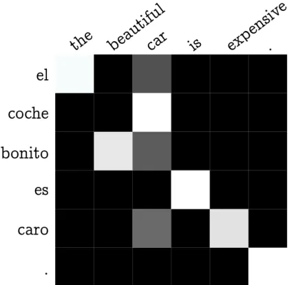
The proposal arises from the fact that word order and syntax are almost identical for related languages such as Catalan and Spanish. After the analysis of attention matrices outputted by TensorFlow’s nmt project using both Bahdanau’s and Luong’s attention it was confirmed that as expected, when translating English into Spanish (Fig. 4.1), the attention mechanism is clearly helping the network to pay attention to the correct part of the sentence, usually more than one word, at each time-step.

(33)

the beautiful

car

is

exp

ensiv

.

e

el

coche

bonito

es

caro

.

Figure 4.1: English to Spanish Attention Matrix

In this graphic representation of a matrix containing all attention vectors containing all αij,

the lighter the color the higher the α factor is, and therefore, the more attention is payed to the input word on the top while outputting the word on the left.

While executing an inference example on TensorFlow’s nmt’s standard configuration with bidi-rectional encoder and Luong attention the content of the variable storing all αij values around

the line 1415 of the file attention wrapper.py was printed. Then, those values are represented using matplotlib’s function matshow obtaining Fig. 4.1.

In this image, it is easy to see how the attention matrix is “paying attention” to the word “car” not only when outputting the word “coche” but also when outputting the words “El”, “bonito” and “caro”. This is because the attention matrix directs part of the attention to “car”, which carries information about gender and number. In addition to this, as shown with the words “beautiful car” and “coche bonito”, the attention matrix also shows how word order is taken into account and helps the network pay attention to the third input word when outputting the second word, as common grammatical structures in English like article+adjective+noun are different in Spanish, where it is article+noun+adjective.

(34)

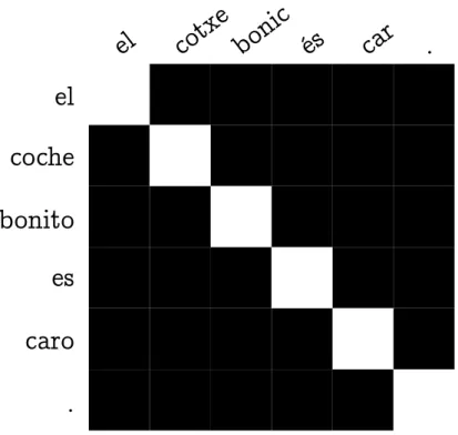
However, as shown in Fig. 4.2, Catalan to Spanish translation shows a very different use of the attention matrix.

el

cotxe bonic és

car

.

el

coche

bonito

es

caro

.

Figure 4.2: Catalan to Spanish Attention Matrix

In most Catalan to Spanish translations’ attention matrices it is easy to observe two main char-acteristics (described below) closely related to the two main “uses” described for the attention mechanism in Section 2.6.

On the other hand, it is also easy to see that when outputting a target word, the attention mechanism is (almost) always paying attention to the source word in its same position (as long both the source and target sentences have the same length): to translate yi the network

(almost) only pays attention to xi and marginally to xi−k and xi+k where k ≥1.

These two characteristics make outputted attention matrices look almost as an empty (black) attention matrix except for the full (white) diagonal and gray adjacent positions as seen in Fig. 4.3.

(35)

el

coc

he

azul

es

.

el

cotxe

és

blau

.

bonito

bonic

Figure 4.3: Spanish to Catalan translation

In this case the attention is not completely payed to the diagonal, as attention needs to be payed to “coche” to produce the target word “blau” because the source word “azul” does not

contain information about its gender.

Taking into account that the attention matrices produced by the attention mechanism have similar characteristics every time a translation is performed between related languages and that its characteristics are recreatable a priori, the next step to simplify the architecture is creating a synthetic attention matrix for the decoder to use. To accomplish this, a Gaussian approach is followed to determine how much attention to pay to each source word when outputting a target word.

By studying the attention matrices outputted, it has been determined that both Bahdanau’s and Luong’s attention mechanisms tested on TensorFlow’s nmt project trained with a mix of two corpora (Diari Oficial de la Generalitat de Catalunya and elPeri´odico, totaling about 7 million sentences) end up paying most of the attention to the source word in the same position as the current target word, and the rest of the attention is gradually distributed among the adjacent words, a normal distribution with a small bell width can be used to mimic this, as illustrated in Fig. 4.4.

(36)

Figure 4.4: Attention vectors with gaussian distribution

This figure shows attention vectors with a Gaussian distribution centered in different positions, the bell’s width will be determined later.

As the functions responsible of implementing Bahdanau’s and Luong’s attention mechanism are external to TensorFlow’s nmt project (which makes use of numerous external libraries, most of them provided by TensorFlow) the functions that needed to be reimplemented are in TensorFlow’s standard machine translation library file attention wrapper.py. There, a new class GaussAttention was created with the same public interface as BahdanauAttention and LuongAttention inhereting from the AttentionMechanism parent class, where the previously im-plemented function tf_createVector is called. This new function, called inside the new class GaussAttention inside TensorFlow’s attention wrapper.py file, returns vectors of the same size as the input sentence, and filled with a normal Gaussian distribution centered in the same position as the target word being outputted. This new function is called as shown bellow:

attention_vector = ops.convert_to_tensor(create_vector.tf_createVector( math_ops.cast(array_ops.size(self._keys[0])/128, dtypes.int32), time))

(37)

The function tf_createVector2 called in the code above, outputs a vector of a certain size filled with a normal distribution centered in a certain position, self._keys[0]/128is the size of the input sentence being translated, and therefore the size of the attention vector to be created and time is the position of the target word being translated in this time-step, hence where the bell peak will be positioned. Due to the limited scope of this work, the fact that most translations between Catalan and Spanish have the same number of words and the complexity of proceeding otherwise, this project does not take into account the uncommon sentences that have different number of words in source and target language.

def tf_createVector(vectorSize, mainWord):

init = tf.TensorArray(dtype=tf.float32, size=0, dynamic_size=True) result = tf.TensorArray(dtype=tf.float32, size=0, dynamic_size=True) total = tf.constant(0.0)

_, aux, _, _, total = tf.while_loop(cond, body, [vectorSize, init, 0, mainWord, total])

stackedAux = aux.stack()

_, finalResult, _, _, _ = tf.while_loop(cond2, body2, [vectorSize, result, stackedAux, 0, total])

return [finalResult.stack()]

Where cond, cond2, bodyand body2 are functions described bellow:

(38)

def cond(vectorSize, output, i, mainWord, total): # i < vector size

return tf.less(i, vectorSize)

def cond2(vectorSize, result, output, i, total): # i < vector size

return tf.less(i, vectorSize)

def body(vectorSize, output2, i, mainWord, total): # gets gauss value at a certain position of the bell

tmp = tf_gauss(a, b, c, tf.subtract(i, mainWord)) output2 = output2.write(i, tmp)

return vectorSize, output2, i+1, mainWord, total+tmp

def body2(vectorSize, result, output, i, total): # normalizes values to add up to 1

result = result.write(i, output[i]/total) return vectorSize, result, output, i+1, total

Where tf_gauss is the TensorFlow language implementation equivalent to the Gaussian dis-tribution formula:

f(x) = ae−(x2−cb2)2

that returns a Gaussian value given the parametersa,b, c(bell height, peak position and bell width) and x.

(39)

def tf_gauss(a, b, c, x):

base = tf.subtract(tf.cast(x, tf.float32),tf.constant(b)) multiplier = tf.pow(base, tf.constant(2.0))

numerator = tf.constant(-1.0, dtype=tf.float32)* multiplier denominator = tf.multiply(2.0, tf.pow(c, tf.constant(2.0))) return tf.multiply(a, tf.exp(tf.cast(

numerator / denominator, tf.float32)))

Parametera, bell height, is kept constant at any value, in this case 1 was chosen, as the Gaussian values contained in vector aux are normalized so that all values contained sum 1 in vector

f inalResult. Parameter b, peak position, is kept at 0 so there is no offset in the distribution and parameter c, bell width, with values ranging between 0 and 1, will be determined in experimental tests explained in Section 5.3.1. Parameter x, where the bell’s maximum is situated, is the position of the target word being outputted.

The function tf_createVector returns vectors like the ones shown in Fig. 4.5 when executed with the bell width indicated in the same figure.

(40)

Bell Width = 0.1

(41)

Chapter 5 Experiments

5.1 Datasets

The datasets used for this work are a combination of the Diari Oficial de la Generalitat de Catalunya1 and elPeri´odico2 parallel corpora.

The resulting parallel corpus has been lower cased (after learning a TrueCase model), tokenized3 and numbers have been substituted by the token <num> using regular expressions. In addition to this, sentences with more than 40 words have been removed and the vocabulary size has been limited to the 30.000 most common words.

The corpus was then divided into the fragments shown in Table 5.1.

Copus Size train 5.5M development 500k rnn test 500k gauss test 56k final test 500k

Table 5.1: Corpora sizes in sentences

1_{http://dogc.gencat.cat/} 2_{https://www.elperiodico.cat/}

3_{https://github.com/moses-smt/mosesdecoder/blob/master/scripts/tokenizer/tokenizer.perl}

(42)

28 Chapter 5. Experiments

Thedevelopmentcorpus was used in the training process to test the quality of the translations

being produced as the training of the network went on. The gauss test corpus was used to test the translation qualities with different bell widths (changing parameter c in the function

tf createV ector). Thef inal test corpus was used to evaluate the resulting simplified network

after being trained and with the Gauss bell width set to the desired value.

5.2 Environment

Throughout all the process of development and testing of this work, the environment (regarding hardware, OS, CUDA and TensorFlow versions, etc) has been kept constant to avoid getting different results for reasons other than voluntary implementation and configuration changes.

For the hardware, we have used Amazon’s cloud computing service AWS, due to their great performing GPUs; an AWS EC2 p2.xlarge instance with the following specifications has been used both for training and inference:

50-100GB storage for training

20-50GB storage for development and testing 61GB RAM

4 vCPUs

NVIDIA Tesla K80 GPU

In order to use the same instance setup every time, an Amazon Machine Image (AMI) was created and saved for every use. Its OS is Ubuntu Server 16.04 LTS with CUDA9.0 and cuDNN7 and a January 10th 2018 nightly version of TensorFlow. The baseline NMT software used is Tensorflow’s nmt project4 _{[Luong et al., 2016], nightly build from January 10th 2018}

too.

(43)

5.3. Experiments 29

5.3 Experiments

A number of experiments have been conducted during the development of this work, apart from the standard network training for TensorFlow’s baseline nmt software, experiments have been carried out to find out which bell width to use when using Gauss attention (discussed in Section 5.3.1) and to determine the difference in translation quality of different simplified versions of the baseline software (discussed in Section 5.3.2).

5.3.1 Bell Width Experiments

To determine the width of the Gaussian bell to use in the Gaussian attention, many different bell widths ranging from 0 to 1 like those shown in Fig. 5.1 were explored and tested. The different translation qualities depending on the bell widths are shown in Fig. 5.2.

c = 0.10 c = 0.25 c = 0.50 c = 0.75

(44)

30 Chapter 5. Experiments 0 . 1 0 . 2 0 . 3 0 . 4 0 . 5 0 . 6 0 . 7 0 . 8 0 . 9 1 0.2 0.24 0.28 0.32 0.36 0.4 0.44

Gauss Bell Width

BLEU

Figure 5.2: Translation qualities with Gaussian attention with different bell widths The scores shown correspond to translations performed using TensorFlow’s nmt project with standard configuration, bidirectional encoder, no beam search and Gaussian attention with different bell widths.

Bilingual evaluation understudy (BLEU) [Papineni et al., 2002] has been used as the metric to evaluate the translation quality partly because of its popularity in other studies. This metrics aims at measuring the degree of similarity between the reference translation and the produced translation by counting how many n-grams are present in both translations.

As seen in Fig. 5.2, the best value for the bell’s width is between 0.25 and 0.4. After trying multiple values ranging from 0.25 to 0.4, 0.3 was determined to be the value for the bell’s width that yields best results when translating between Catalan and Spanish (Fig. 5.3).

(45)

5.3. Experiments 31

This result is not surprising, as this value produces attention vectors with values very simi-lar to those yielded when translating with Bahdanau’s or Luong’s attention mechanisms. It gives almost total attention to the source word in the same position as the target word being outputted, some attention to the adjacent words and only residual attention is payed to the remaining words.

5.3.2 Simplification Experiments

Once the correct bell width was determined, a number of different networks (with different configurations an features) were trained under the same conditions and compared. All com-binations (with or without bidirectional encoder, with or without beam search and without attention, with Gaussian attention or Luong’s attention) were evaluated.

Due to its great results, Luong’s attention has been chosen to be compared against no attention and Gaussian attention.

(46)

Chapter 6 Results & Discussion

After the experiments described in the previous chapter, the results for Catalan-Spanish trans-lation in Table 6.1 were obtained:

# Encoder Beam Attention BLEU Training T. Trans. T. Train. Params.

1 Uni 1 No Attention 0.1365 12h 15m 1h 1m 9,816,485 2 Uni 1 Gaussian 0.4387 14h 15m 1h 4m 9,905,841 3 Uni 1 Luong 0.5803 14h 48m 1h 4m 9,954,623 4 Uni 5 No Attention 0.1477 18h 26m 1h 3m 9,817,740 5 Uni 5 Gaussian 0.4552 20h 44m 1h 8m 9,906,256 6 Uni 5 Luong 0.5773 21h 1h 11m 9,955,734 7 Bi 1 No Attention 0.1581 12h 40m 1h 2m 12,047,109 8 Bi 1 Gaussian 0.4721 14h 57m 1h 5m 12,146,893 9 Bi 1 Luong 0.6072 15h 31m 1h 8m 12,194,412 10 Bi 5 No Attention 0.1764 18h 49m 1h 2m 12,048,488 11 Bi 5 Gaussian 0.5103 22h 36m 1h 10m 12,147,482 12 Bi 5 Luong 0.6018 22h 53m 1h 14m 12,195,945

Table 6.1: Evaluation Results in BLEU

The most immediate conclusions that can be drawn from these results are the similarities in BLEU score, training and translation time and number of trainable parameters between gaus-sian attention and Luong attention when compared to no attention. Note that the substitution of the bidirectional to unidirectional encoder seems to have a greater impact on translation quality than the elimination of beam search. Further analysis is done in Chapter 7.

(47)

Chapter 7 Discussion and Conclusions

From the analysis of the results presented in Table 6.1 a few conclusions can be drawn. First of all, from the difference in BLEU score between the blue and yellow rows, it is easy to conclude that the removal of extra features like beam search and bidirectional encoder from the baseline state-of-the-art implementation, as hypothesized in Sections 4.1 and 4.2, does not seem to have a huge impact on translation quality (about 4 BLEU points). However, this removal does reduce the training time in about 6-8 hours (50-66%) and the number of trainable parameters in more that 2 million (about 20%). After looking at the red and green rows, it is noticeable that both beam search and the bidirectional encoder seem to have a similar effect on the BLEU score although the bidirectional encoder has a much bigger impact on the number of trainable parameters and training time.

With all this in mind, we can therefore say that removing beam search but specially substituting the bidirectional encoder by a unidirectional encoder seems like a good idea for simplifying the network without harming translation quality too much in related-languages-translation situations.

On the other hand, when comparing results from different rows of the same color, an interesting overview of the impact that attention mechanisms have on translation quality can be drawn. Independently of other features like beam search or bidirectional encoder, the use or lack of different attention mechanisms seem to have a constant effect on the BLEU scores obtained,

(48)

34 Chapter 7. Discussion and Conclusions

meaning that results with Gaussian attention obtain about 30 BLEU points more that attention-less configurations, and Luong attention obtains a bit attention-less than 15 points more than Gaussian attention.

When comparing the three different scenarios in relation to attention mechanisms (no use of attention mechanism, use of Gaussian attention mechanism and use of Luong’s attention mechanism) the results indicate that the use of any kind of attention mechanism strongly boosts translation quality, Gaussian attention roughly triplicating its BLEU score while Luong’s attention obtaining roughly 4 times more BLEU score.

But more importantly, Luong’s complex state-of-the-art attention mechanism (based on Bah-danau’s) obtains a score (only) about ∼27% higher than the Gaussian attention proposed in this work. On the other hand, Gaussian attention obtains scores that are approximately 300% (or more) higher than those without attention mechanism at all having only about 1% more trainable parameters.

It is interesting to see how such a simple approach to attention mechanism obtains these results when applied to related languages. Achieving a BLEU score three times higher on a modified network only by adding a simple Gaussian normal distribution to the attention mechanism is a step forward towards simplified and more computational cost-efficient NMT systems.

It is worth noting, that even though the beam of beam search has been reduced to 1 and that Luong’s attention mechanism has been substituted by the newly developed Gaussian attention, due to the high coupling of the baseline project, many of the structures and modules have not been completely removed. So this means that even though beam search and Luong’s attention mechanism are not used at all, many of their processes are still being computed in the background. This translates into an incomplete optimization of the network, this is why a further reduction in trainable parameters and training time is expected if the simplifications described in this work were applied to an uncoupled project or to a new NMT system made from scratch.

(49)

7.1. Future Work 35

7.1 Future Work

During the development of this work, and due to the limited time, resources and scope of this project, a few possible improvements or ideas have been left for future work.

7.1.1 Additional Feature Reduction

Apart from the simplifications performed in this work, other features can always be removed from the state-of-the-art baseline to see what effect this has on its performance. Some ideas could be the difference between BPE and no BPE, the use of LSTM units, GRU units or regular neurons.

These ideas could be interesting, but have been considered not to be too significant in the frame of related language translation.

7.1.2 Execution Time

One of the improvements an NMT recurrent encoder-decoder could benefit from after the sim-plification of its architecture is the significant reduction of the training and inference time. However, in this work, not much time optimization has been achieved due to the baseline’s software’s high coupling. Even though some of the software’s features, like in the case of Bah-danau’s and Luong’s attention, have been somehow disabled and substituted by the proposed Gaussian attention, the elimination of all the background processing that is done to enable Bahdanau’s or Loung’s attention has not been possible without rewriting much of TensorFlow’s source code.

The complete elimination of the features explained in Chapter 4 in order to see its temporal cost reduction is something worth trying in the future.

(50)

36 Chapter 7. Discussion and Conclusions

7.1.3 Test the Resulting Architecture with Other Languages

The performance of the simplified architecture proposed in this work is extensively tested and reported in Chapters 5 and 7 and in Section 6.1. Nevertheless, testing the performance of these simplifications with the translation of language pairs different from the ones the simplifications were intended for could be very interesting.

This could be really interesting to see how much of the benefit explored in this work is really due to the similarity between related languages and how much can be generally applied to any NMT situation.

Therefore, evaluating the translation quality of the proposed system with language pairs like Spanish-English or German-Catalan could be an interesting idea for future work.

(51)

Appendix A

Project Work

Throughout the development of this project as well as the previous research phases and the later results evaluation and reporting, many tasks have been performed and a lot of new knowledge has been acquired. The different tasks and researches performed for this work are described in this appendix.

A.1 Understanding NMT Recurrent Encoder-Decoder

Architecture

Before starting the development process, a long learning process was carried out in order to understand state-of-the-art NMT recurrent encoder-decoder architectures and some of the fea-tures that are many times used in NMT systems. This goes from understanding the internal behavior of recurrent neural networks, to understanding how attention mechanisms work, what the vanishing gradient issue is, or how embeddings represent a word’s meaning in a contextual similarity vectorial space.

(52)

38 Appendix A. Project Work

A.2 Programming with TensorFlow

The next phase, before starting the development of the new system, was to learn how to program in TensorFlow. Although TensorFlow is based on Python, a very different paradigm is used. The idea of nodes is completely present in the way TensorFlow code is programmed. Every action is coded into a neuron which has to be called (used) in order to be executed. This makes programming quite challenging when one is used to the imperative or functional paradigms. Simple actions such as printing a small output or multiplying two numbers is much more complex than expected and therefore needed some training before developing the final simplified system.

A.3 Using Amazon Web Services instances

As stated in Section 5.2, Amazon’s cloud computing service Amazon Web Services (AWS) has been used throughout the development and evaluation of this project. Therefore, a deep understanding of how Amazon’s instances work was needed. In order to save money, spot instances were used. These instances are a sort of auction instances, where a maximum price you are willing to pay is set, and then you are allowed to use the preferred instance paying the current price (which is updated constantly, and usually lower than the normal fixed-priced instances) as long as the current price does not exceed the selected maximum price you are willing to pay.

A.4 Corpora Management and Tokenization

For the development and testing of the system proposed in this work, many experiments have been conducted, most of which needed the use of parallel corpora. Because of this, dealing with corpora, regarding downloading, separating them into different chunks, tokenization, filtration, etcetera, has been necessary. Determining the vocabulary size and the maximum sentence

(53)

A.5. Scientific Analysis 39

length allowed have also been tasks which have been performed regarding corpora.

A.5 Scientific Analysis

For most of the tests performed during the development phases and during the final evaluation phase, many experiments have been conducted, and therefore, scientific methodologies have been applied in order to get accurate results. This implied using separate corpora for each test, testing each configuration independently to see their performance, analyzing the results obtained, etc.

(54)

References

[Artetxe et al., 2017] Mikel Artetxe, Gorka Labaka, Eneko Agirre, Kyunghyun Cho. Unsuper-vised Neural Machine Translation. Conference paper at ICLR 2018. 2017

[Bahdanau et al., 2014] Dzmitry Bahdanau, Kyunghyun Cho, Yoshua Bengio. Neural Machine Translation by Jointly Learning to Align and Translate. 2014.

[Chalmers, 1990] Chalmers, D.J. (1990) Syntactic Transformations on Distributed Represen-tations, Connection Science 2:12, 5362.

[Cho et al., 2014] Kyunghyun Cho, Bart van Merrienboer, Caglar Gulcehre, Dzmitry Bah-danau, Fethi Bougares, Holger Schwenk, Yoshua Bengio. Learning Phrase Representations using RNN Encoder-Decoder for Statistical Machine Translation. 2014

[Chrisman, 1991] Chrisman, L. (1991) Learning Recursive Distributed Representations for Holistic Computation, Connection Science 3:4, 345366.

[Chung et al., 2014] Junyoung Chung, Caglar Gulcehre, KyungHyun Cho, Yoshua Bengio. Em-pirical Evaluation of Gated Recurrent Neural Networks on Sequence Modeling. 2014

[Freitag and Al-Onaizan, 2017] Markus Freitag, Yaser Al-Onaizan. Beam Search Strategies for Neural Machine Translation. 2017

[Hochreiter., 1991] Sepp Hochreiter. Untersuchungen zu dynamischen neuronalen Netzen. 1991

[Hochreiter, Schmidhuber, 1997] Sepp Hochreiter and Jrgen Schmidhuber. Long Short-Term Memory. 1997

(55)

REFERENCES 41

[Hochreiter et al., 2001] S. Hochreiter, Y. Bengio, P. Frasconi, and J. Schmidhuber. Gradient flow in recurrent nets: the difficulty of learning long-term dependencies. 2001

[Huang et al., 2017] Liang Huang, Kai Zhao and Mingbo Ma. When to Finish? Optimal Beam Search for Neural Text Generation (modulo beam size).

[Kalchbrenner and Blunsom, 2013] N. Kalchbrenner, P. Blunsom. Recurrent Continuous Trans-lation Models. Proceedings of the 2013 Conference on Empirical Methods in Natural Lan-guage Processing. 2013

[Koehn and Knowles, 2017] Philipp Koehn and Rebecca Knowles. Six Challenges for Neural Machine Translation. Proceedings of the First Workshop on Neural Machine Translation. 2017

[Luong et al., 2016] Minh-Thang Luong, Hieu Pham, Christopher D. Manning. Effective Ap-proaches to Attention-based Neural Machine Translation. 2015.

[Luong et al., 2016] Thang Luong, Eugene Brevdo, Rui Zhao. TensorFlow Neural Machine Translation (seq2seq). https://github.com/tensorflow/nmt#neural-machine-translation-seq2seq-tutorial. 2016.

[ ˜Neco and Forcada, 1997] ˜Neco, R. P., Forcada, M. L. (1997, June). Asynchronous translations with recurrent neural nets. In Neural Networks, 1997., International Conference on (Vol. 4, pp. 25352540). IEEE.

[Papineni et al., 2002] Papineni, K.; Roukos, S.; Ward, T.; Zhu, W. J. (2002). BLEU: a method for automatic evaluation of machine translation. ACL-2002: 40th Annual meeting of the Association for Computational Linguistics

[Reynolds, A. Craig, 1954] Reynolds, A. Craig. The conference on mechanical translation. Me-chanical Translation. 1954

[Sutskever, Vinyals and Le, 2014] Ilya Sutskever, Oriol Vinyals, Quoc V. Le. Sequence to Se-quence Learning with Neural Networks. 2014

(56)

42 REFERENCES

[Sutskever et al., 2014] Ilya Sutskever, Oriol Vinyals, Quoc V. Le. Sequence to Sequence Learn-ing with Neural Networks. 2014

[Witten et al., 1994] Ian H. Witten, Alistair Moffat, and Timothy C. Bell. Managing Gigabytes. New York: Van Nostrand Reinhold, 1994

Simplifying Encoder-Decoder-Based Neural Machine Translation Systems to Translate between Related Languages

Trabajo Fin de Grado

Simplifying

Encoder-Decoder-Based

Neural Machine Translation

Systems to Translate between

Related Languages

Universidad de Alicante

Escuela Polit´ecnica Superior

Departamento de Lenguajes y Sistemas Inform´

aticos

Simplifying Encoder-Decoder-Based Neural

Machine Translation Systems to Translate

between Related Languages

Lucas Gil Melby

Abstract

Acknowledgements

Contents

List of Tables

List of Figures

Chapter 1

Introduction

Chapter 2

Encoder-Decoder Recurrent

Architecture for NMT

2.1

Encoder-Decoder NMT Overview

2.2

LSTM and GRU Units

LSTM

GRU

2.3

Word Embeddings

2.4

Bidirectional Encoder

c

2.5

Beam Search

2.6

Attention Mechanism

h

h

That

h

h

house

h

h

is

h

h

very

h

h

expensive

h

h

.

⊕

s

s

muy

cara

...

...

α

α

α

α

α

α

c

the house is

very exp

ensiv

e

.

Chapter 3

Motivation and Objectives

Chapter 4

_α

_α

_α