Tests of Markov Order and Homogeneity in a Markov Chain

Research Report

2011:7

ISSN 0349-8034

Mailing address: Phone Home Page:

Statistical Research Unit Nat: 031-786 00 00 http://www.statistics.gu.se/

P.O. Box 640 Int: +46 31 786 00 00

SE 405 30 Göteborg Sweden

Research Report

Statistical Research Unit

Department of Economics

University of Gothenburg

Sweden

Tests of Markov Order and Homogeneity in a

Markov Chain Model for Analyzing

Rehabilitation

Research Report

2011:7

ISSN 0349-8034

Mailing address: Phone Home Page:

Statistical Research Unit Nat: 031-786 00 00 http://www.statistics.gu.se/

P.O. Box 640 Int: +46 31 786 00 00

SE 405 30 Göteborg Sweden

Tests of Markov Order and Homogeneity in a Markov Chain

Model for Analyzing Rehabilitation

ROBERT JONSSON

Department of Economics, Goteborg University, Box 640, 405 30 Goteborg, Sweden

Abstract. A three-state non-homogeneous Markov chain (MC) of order m≥0, denoted M(m), was previously introduced by the author. The model was used to analyze work resumption among sick-listed patients. It was demonstrated that wrong assumptions about the Markov order m and about homogeneity can seriously invalidate predictions of future health states. In this paper focus is on tests (estimation) of m and of homogeneity. When testing for Markov order it is suggested to test M(m) against M(m+1) with m sequentially chosen as 0, 1, 2,…, until the null hypothesis can’t be rejected. Two test statistics are used, one based on the Maximum Likelihood ratio (MLR) and one based on a chi-square criterion. Also more formal test strategies based on Akaike’s and Baye’s information criteria are considered. Tests of homogeneity are based on MLR statistics. The performance of the tests is evaluated in simulation studies. The tests are applied to rehabilitation data where it is concluded that the rehabilitation process develops according to a non-homogeneous Markov chain of order 2, possibly changing to a homogeneous chain of order 1 towards the end of the period.

1. Introduction

In an earlier paper the author introduced a three-state Markov chain (MC) model for analyzing the progress of patient’s health [9]. The states were denoted 2, 1 and 0 and represented the development from ‘Acute diseased’ to ‘Improved’ and further to ‘Healthy’. Another example is progression through the stages: HIV infection, AIDS and finally death. The MC model is allowed to be non-homogeneous in discrete time and also to have any Markov order m, where m refers to the number of time points back in history that has to be considered when assigning a transition probability one step ahead. In [9] it was demonstrated that assuming homogeneity, when the MC actually is non-homogeneous, can seriously invalidate calculations of predictive probabilities two or more steps ahead. It was also demonstrated that prediction probabilities are heavily dependent on the choice of m.

Although correct specifications of both heterogeneity and of Markov order are of crucial importance for the analysis, few attempts have been made to compare and evaluate various tests that can be used in order to find a proper structure of the MC. In these respects one may notice a difference between various disciplines. Econometricians have since long ago used non-homogeneous MC models, or models with time varying transition probabilities in their terminology (see e.g. Diebold et. al. [ 3] and Van den Berg [14]). However, the latter seem to only cover the case m = 1. Among statisticians oriented toward natural sciences focus has been on testing for a proper value of m in homogeneous MCs ([7], [2], [10], [11]), with a few exceptions (see e.g. [8]).

In this paper various tests of Markov order and of homogeneity are considered in the three-state MC and the performances of the tests are studied in Monte Carlo simulations. The methods are then applied to data of work resumption after rehabilitation. The paper ends with a concluding discussion. Throughout the paper the notation M(m) will be used for a MC of order m.

2. Assumptions, notations and some basic results

Let ( )

, 1, 2,..., m

t

X t= T denote the health state at time t for a MC of order m, with the possible outcomes 0 (Healthy), 1 (Improved) and 2 (Acute diseased). The probabilities of these

outcomes are ( )

( m ), 0,1, 2 t

P X = j j= . At t=1 only the states 1 and 2 are available and for these initial states the notations π =₂ P X( ₁( )m =2) and 1−π₂ = P

(

X₁(m) =1

)

are used. From one state at time t to the following state at time t+1 only the following transitions are possible: 2_t →(2_t+1 or 1 ), 1_{t+1 t} →(1 or 0 ) and 0_{t+1 t+1 t} →0_t+1. Here the notation j_t has been used to denote that state j is occupied at time t. Transitions to state 2 can thus only take place from state 2. Therefore, omitting the index m for simplicity,

(

t 1 2 t s 2 t 2

) (

t 1 2 t 2

)

t

P X ₊ = X ₋ = X = =P X₊ = X = =β (1)

(

t 1 1 t s 2 t 2

) (

t 1 1 t 2

)

1 t

P X ₊ = X ₋ = X = =P X ₊ = X = = −β

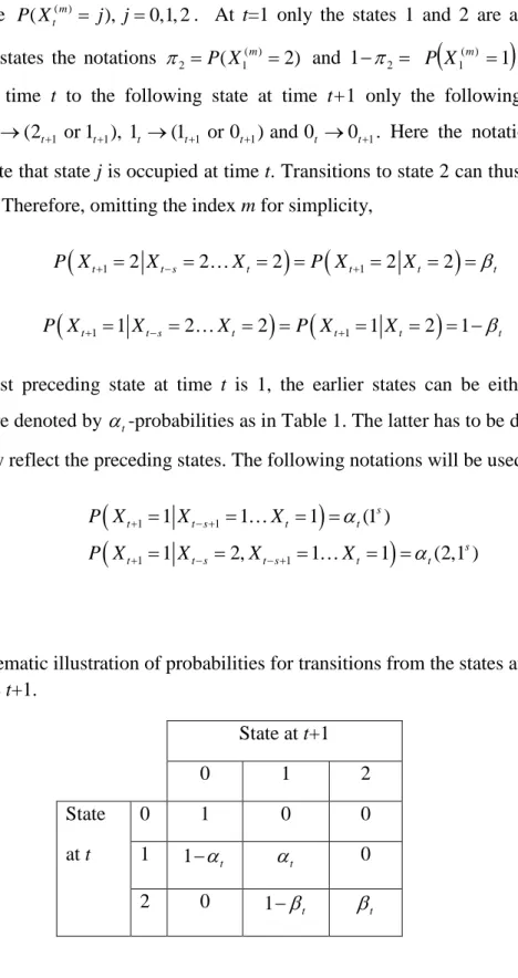
When the last preceding state at time t is 1, the earlier states can be either 1 or 2. Such transitions are denoted by α_t-probabilities as in Table 1. The latter has to be denoted in such a way that they reflect the preceding states. The following notations will be used:

(

)

(

)

1 1 1 1 1 1 1 (1 ) 1 2, 1 1 (2,1 ) s t t s t t s t t s t s t t P X X X P X X X X α α + − + + − − + = = = = = = = = =   (2)

Table 1 Schematic illustration of probabilities for transitions from the states at time t to the states at time t+1. State at t+1 0 1 2 State 0 1 0 0 at t 1 1−α_t α_t 0 2 0 1−β_t β_t

In general, let (i_sj_t)denote the event that a sequence of states is occupied, from state i at time s to state j at time t. In analogy with the notations for the transition probabilities in (1) and (2) which were designated by Greek symbols, the following notations are used for the transition frequencies:

1

1 t+1

1 t+1

Number of transitions from (2 ) to (2 ). (1 ) -"- (1 1 ) to (1 ) (2,1 ) -"- (2,1 1 ) to (1 ) t t t s t t s t s t t s t B A A + − + − + = = =   (3)

The state frequencies or risk masses, i.e. the number of persons being in a state just before transitions occur, are denoted in the following way:

1 1 (2) Number of persons in state 2

(1 ) -"- (1 1 ) (2,1 ) -"- (2,1 1 ) t t s t t s t s t t s t N N N − + − + = = =   (4)

The quantities in (3) and (4) are related. If no subjects in the sample disappear between the transitions, then e.g.Bt = Nt+1(2). Since withdrawals may occur in practice both notations in (3) and (4) will be used. The total fixed sample size is denoted by n. An illustration of these frequencies is shown in Table 2 for a Markov chain of order m=2, or M(2). Here one may

notice that 2 2

(1 ) (2,1) (1) and (1 ) (2,1) (1)

t t t t t t

A +A =A N +N =N .

Table 2 Transition- and state frequencies in the three-state model for progress of health when the Markov order is m=2.

State at t+1 0 1 2 Total (0,0) N_t(0) 0 0 N_t(0) State at (1,1) 2 2 (1 ) (1 ) t t N −A At(1 )2 0 2 (1 ) t N (t-1,t) (2,1) N_t(2,1)−A_t(2,1) A_t(2,1) 0 N_t(2,1) (2,2) 0 N_t(2)−B_t B_t N_t(2) n

The random marginal quantities to the right in Table 2 will in the sequel be termed working sample sizes and these will be used for estimating the α and β parameters.

The likelihood L( )m of all observations in the three-state model of Markov order m is rather complicated and an expression is therefore omitted here and is given in the Appendix A1. (See also [9] for some special cases.) The ML estimators of the parameters are easily found from the likelihood,

ˆ _, (2) t t t B N β = ˆ (1 ) (1 ) (1 ) s s t t s t A N α = , ˆ (2,1 ) (2,1 ) (2,1 ) s s t t s t A N α = (5) In the homogeneous case,

1 1 1 1 ˆ (2) T t t T t t B N β − = − = =

∑

∑

, 1 1 (1 ) ˆ (1 ) (1 ) T s t s t s T s t t s A N α − = − = =

∑

∑

, 1 1 (2,1 ) ˆ (2,1 ) (2,1 ) T s t s t s T s t t s A N α − = − = =

∑

∑

(6)

The above relations hold only for the case m≥1. Whenm=0 (independent transitions)

(

1t 11t

) (

1t 1 2t

)

P ₊ =P ₊ , from which it follows that α_t(1)+β_t =1. By putting this relation into the Likelihood one easily gets the following ML estimate of α_t(1) (under independency denoted α_t) (1) (2) ˆ (1) (2) t t t t t t A N B N N α = + − + (7)

In the homogeneous case the index t is dropped from the parameter and all terms in the numerator and denominator are preceded by a summation symbol, just as in (6).

Some properties of the estimators in (5)-(7) are discussed in [9]. It can be shown that they are unbiased, but the variances of the estimators do not behave as in the case where the sample sizes in the denominators are fixed quantities.

3. Tests of Markov order

In this section, first some test statistics based on the Maximum Likelihood Ratio (MLR) ( , *) ( ) ( *)

ˆ m m ˆm _/ ˆm

L L

Λ = are presented for testing M(m) against M(m*), m < m* Focus will be on the case m* =m+1, with m sequentially chosen as 0,1,2,… . The process is repeated until H0 can’t be rejected. This strategy is different from the one recommended by Hoel [7], where it is

instead advocated to start with a large value of m and test successively for lower order. Hoel’s approach may be risky because tests of larger values of m are based on more estimated parameters of lower precision due to smaller working sample sizes. This in turn decreases the power of the tests and opens for the possibility that a large value of m is falsely accepted. Various test strategies are discussed in Section 3.3 below.

The case m = 0 (independency) is considered first, followed by more general cases. It will be assumed that the sample sizes are so large that −2 lnΛˆ has a chi-square distribution under H0, with degrees of freedom (df) equal to the difference between the number of estimated parameters under H0 and H1 (cf. Ch. 22.7 in Stuart et al. [13]). Also an alternative chi-square procedure for testing M(m) against M(m+1) is presented. Finally some criteria for estimating a proper Markov order are discussed. Throughout this section focus will be on heterogeneous MCs. Expressions for the homogenous case are obtained by simply dropping the indices of the estimated parameters and by performing a summation over all frequencies.

3.1 Maximum Likelihood Ratio tests of M(m) against M(m+1)

Consider first test of M(0) against M (1). From the Likelihood given in Appendix A1 it is easily shown that the MLR statistic based on transitions from time i to time i+1, i =1…T-1 can be written ) 1 ( ) 1 ( ) 2 ( ) 1 ( ) 1 , 0 ( ) 1 ( ˆ 1 ˆ 1 ˆ 1 ˆ ) 1 ( ˆ ˆ ˆ ˆ 1 ˆ i i i i i i N A i i B N i i A i i B i i i − −       − −         −               − = Λ α α β α α α β α (8)

Here the parameter estimates are given in (5)-(7). Under H0, −2 lnΛˆ(0,1)t has an asymptotic 2

(1)

χ -distribution and H0 is rejected at the 5 % level if −2 lnΛˆt(0,1)exceeds the 95 % percentile of the χ(2)(1)-distribution. When the same hypothesis is tested for a sequence of transitions from time s≥1 to time t≤ −T 1 the MLR-statistic is

∏

= Λ = Λ t s i i t s ) 1 , 0 ( ) 1 , 0 ( , ˆ ˆ ₍₉₎

Now H0 is rejected at the 5 % level if −2 lnΛˆ(0,1)s t, exceeds the 95 % percentile of the 2

(t s 1)

In the homogeneous case the statistic corresponding to (9) is ∑ ∑       − − ∑ ∑       − ∑       − ∑       = Λ − − i i i i i i i i i i i i B N B N B A t s ) 1 ( ) 2 ( ) 1 ( ) 1 , 0 ( , ) 1 ( ˆ 1 ˆ 1 ˆ 1 ˆ ˆ ˆ 1 ) 1 ( ˆ ˆ ˆ α α β α β α α α (10)

Under H0 −2lnΛˆ(s0,,t1)now has a (1) 2

χ -distribution.

The MLR test statistic based on transitions from time i to time i +1, i = m+1…T-1, for testing M(m) against M(m+1), m≥1, in the non-homogeneous case can be expressed as

) 1 , 2 ( ) 1 , 2 ( ) 1 , 2 ( ) 1 ( ) 1 ( 1 ) 1 ( 1 ) 1 , ( ) 1 , 2 ( ˆ 1 ) 1 ( ˆ 1 ) 1 , 2 ( ˆ ) 1 ( ˆ ) 1 ( ˆ 1 ) 1 ( ˆ 1 ) 1 ( ˆ ) 1 ( ˆ ˆ 1 1 1 m i m i m i m i m i m i N A m i m i A m i m i A N m i m i A m i m i m m i − − + + +       − −             − −       = Λ + + + α α α α α α α α (11)

The expression in (11) is obtained after simple but somewhat tedious calculations where the relations (1 ) (2,1 ) 1(1 )and (1 1) (2,1 ) (1 ) 1 m i m i m i m m i m i A A N N N

A + + = + + = have been used.

Under H0, −2lnΛ(im,m+1)has an asymptotic (1) 2

χ -distribution. When the hypothesis is tested for a sequence of transitions from time s≥m+1 tot ≤T −1the MLR statistic is analogous to that in (9) and has the same asymptotic distribution. The test statistic in the homogeneous case is obtained in the same way as in (10).

A general expression of Λˆ(_im,m*)for testing M(m) against M(m*), m < m*, is given in the Appendix A2.

3.2 An alternative test of M(m) against M(m+1)

A test of Markov order 0 against 1 can be based on the difference between ˆ (11) t

α in (5) and ˆ_t

α in (7). For m≥1 a test of Markov order m against m+1 may be based on the differences be

) 1 ( ˆ ) 1 , 2 ( ˆ or ) 1 ( ˆ ) 1 ( ˆ 1 m t m t m t m t α α α α + − −

. In Appendix A3 it is shown that both differences can be expressed in terms of αˆ_t(1m+1)−αˆ_t(2,1 )m . Under H0: M(m), m≥1, the latter quantity has mean 0. Since

(

At(1m 1) Nt(1m 1)

)

+ +

and

(

At(2,1 )m Nt(2,1 )m

)

are independent it follows that a roughly unbiased estimator of 1

ˆ ˆ

( t(1m ) t(2,1 ))m

V α + −α under H0 is given by (see Lemma (c) in Section 3.3 in [8]

(

)

1 1 1 1 0 1 1 ˆ ˆ( (1 ) ˆ (2,1 )) ˆ (1 ) 1 ˆ (1 ) (1 ) (2,1 ) , (1 ) (2,1 ) ˆ where (1 ) (1 ) (2,1 ) m m m m m m t t t t t t m m m t t t m m t t V N N A A N N α α α α α + − + − + +   − = _ − _ + + = + (12)

It follows that a test of Markov order m against m+1, m≥1, can be based on the statistic

1 2 2 1 0 ˆ ˆ [ (1 ) (2,1 )] ˆ ˆ( (1 ) ˆ (2,1 )) m m t t t _{m m} t t X V α α α α + + − = − , (13a)

where the variance in the denominator is given in (12). Under H0, Xt2 is asymptotically distributed as a chi-square variable with df=1.

By similar arguments it follows that a test of M(0) against M(1) can be based on

(

)

2 2 [ˆ (1) ˆ ] (2) ˆ (1 ˆ ) (1) (1) (2) t t t t t t t t t X N N N N α α α α − = − ⋅ + , (13b)

where ˆα_tis given in (7), and 2 t

X has the same asymptotic distribution as in (13a).

3.3 Test strategies

The various tests in the preceding sections give no clear-cut answer to the problem of what Markov order to chose in a given situation. One way to deal with the problem is to perform all possible tests ofM(m)against M(m*), for 0≤ <m m*, where m* is some more or less arbitrarily chosen upper limit for the Markov order. This strategy was used by Gabriel and Neumann [4] when analyzing the frequently quoted Tel Aviv precipitation data, and they drew the conclusion that m=1. No study seems to have been published, where the benefit of such a multiple hypothesis strategy is evaluated. When the number of tests involved is large it is clear that there is a risk of obtaining biased estimates of m.

For a large value of the Markov order the number of parameters to estimate increases rapidly. So, in small samples it is especially important that m is small. In the latter situation one may use the strategy mentioned in the beginning of Section 3 to sequentially testing for higher and higher Markov orders. More formal strategies are Akaike’s information criterion (AIC) (Akaike [1]) and Baye’s information criterion (BIC) [12]. A convenient formulation of

AIC and BIC is the following [10]. Consider the sequence of MLR statistics, Λˆ( ,m m*), for testing M(m) against M(m*) m=0,1,,m*−1. Let df m m( , *)be the df of the test and put

* * ( , ) * ( , ) * ˆ ( ) 2 ln 2 ( , ) ˆ ( ) 2 ln ln( ) ( , ) m m m m AIC m df m m

BIC m sample size df m m

= − Λ −

= − Λ − ⋅ (14)

The estimate of m based on AIC, ˆm_AIC, is chosen such that AIC m(ˆ_AIC)=minAIC m( ), while the estimate based on BIC, ˆm_BIC, is similarly obtained from BIC m(ˆ_BIC)= minBIC m( ). The only difference between AIC m( ) and BIC m( )is that different penalty functions are used, and it is seen that AIC m( )>BIC m( )for sample sizes larger than 8. In the case when transitions are possible to all states, ‘sample size’ in (14) is simply synonymous with n, the total sample size. In the presentmodel it will be clear from the simulation study in Section X that ‘sample size’ should be put equal to the working sample size (cf. Section 2).

The asymptotic properties of AIC- and BIC criteria are well known when applied to Markov chains. The AIC criterion has been proved to be inconsistent as the sample size tends to infinity and overestimates the true Markov order, while BIC is consistent [10]. In finite samples the picture is somewhat unclear. For the Tel Aviv precipitation data mentioned above, Gates and Tong [5] obtained ˆm_AIC =2 while Katz [9] got ˆm_BIC =1, both using *

3

m = . In the last cited study simulations of a two-state Markov chain were performed with m=1. The AIC- and BIC criteria were then applied simultaneously in order to estimate m from samples of various sizes. It was found that both criteria gave estimates of m that were heavily dependent on the sample size. In small samples both criteria suggested the estimates ˆm=0 with highest probability. As sample sizes increased both criteria tended to favor the estimate

ˆ 1

m= . But this process went slower for the BIC criterion than for the AIC criterion. In fact, sample sizes of 1000 and more were needed in order for the BIC criterion to give the estimate

ˆ 1

m= the highest chance, while the AIC criterion only required sample sizes of 300 and more. Thus, although BIC seems to work better than AIC in very large samples, it is not clear that this is the case in small sample cases.

4. Tests of homogeneity

When facing the problem whether a MC is homogeneous or not, it is a good advice to first plot estimates of the various transition probabilities against time, as in Figure 2 in [9]. Such a plot may be accompanied by a table showing the results from tests of homogeneity in an

interval from time u to timev,1≤u<v≤T −1. An example of the latter is given in Table 11 of Section 6. Let any subset of

[

1,...,T −1

]

be denoted by S. Test of homogeneity can be performed for the parameters β_t ,α_t(1s) and α_t(2,1s). Below the MLR statistics for these tests are given.

S t t t = against H : ≠ for ∈ : H₀ β β ₁ β β

By inserting the estimators in (5) and (6) into the likelihood given in Appendix X one gets the MLR-statistic S t t B N t B t B N B t t t t t t t t t ∈ − ∑ ∑ − ∑ = Λ

∏

− − , ) ˆ 1 ( ˆ ) ˆ 1 ( ˆ ˆ ) 2 ( ) 2 ( β β β β (15)

Under H0 −2lnΛˆ has an asymptotic chi-square distribution. The degrees of freedom (df) is the difference between the number of estimated parameters in the numerator and denominator. E.g. if S =

[

1,...,T −1

]

then df is (T-1)-1 = T-2.

( ) ( )

s s _t s

( )

s t S

t 1 = 1 against H : (1 )≠ 1 for ∈ :

H₀ α α ₁ α α

The MLR statistic now becomes

( )

( )

_[

_{( )}

_]

( ) ( )

( )

( )

_[

_{( )}

_]

( ) ( ) t S t A N s t A s t A N s A s s t s t s t t s t t s t t s t ∈ − ∑ ∑ − ∑ = Λ

∏

− − , 1 ˆ 1 1 ˆ 1 ˆ 1 1 ˆ ˆ 1 1 1 1 1 1 α α α α (16)

In this case the largest subset S is

[

s,...T −1

]

in which case df in the asymptotic chi-square distribution is T −s−1. Test of homogeneity of α_t

( )

2,1s is performed in a similar way.

5. Comparative simulation studies

The performance of the various tests that were presented in Sections 3-4 will be studied by simulations. First, the conditions under which the simulations were carried out are given. Then results about the power of some tests of Markov order are presented, followed by a section where the AIC and BIC procedures in Section 3.3 are compared. Finally, the power functions of the proposed tests of homogeneity are studied.

5.1 Design of the simulation studies

Tests of Markov order were applied to the following cases: M(0) against M(1), M(0) against M(2) and M(1) against M(2). The tests were studied by simulating realizations of X_t( Cf. Section 2.) for t =1,...,4. Frequencies of the original state X₁were obtained by assigning the states 2 and 1 to each subject in a sample of size n with probabilities π₂ and1−π₂, respectively. n was chosen as 100, 200, 500 and 1000 whereas π₂was 0.5 and 0.9. The probabilities β_tof remaining in state 2 were β₁ =0.60,β₂ =0.65andβ₃ =0.70. When testing M(0) against M(1) the probability that a subject remains in state 1 was chosen as

) 1 ( 1 ) 1 ( β δ αt = − t + . Here 0 ) 1 ( ₌

δ corresponds to M(0) or independent transitions whereas

0

) 1 ( ≠

δ gives rise to various M(1)-models. For tests of M(0) against M(2) and M(1) against M(2) the α_t-probabilities were α₁

( )

1 =1−β₁ +δ(1) andfor t=2,3α_t

( )

12 =1−β_t +δ( )12 ,

) 1 , 2 ( 1 ) 1 , 2 ( β δ αt = − t + . Here ( ) ( ) ( ) ( ) 0 models, -M(0) gives 0 1 2,1 1 , 2 12 =δ = δ 2 =δ ≠ δ gives

M(1)-models and δ( )12 ≠δ( )2,1 gives M(2)-models. The values of the δ -parameters that were chosen in the simulations are given in Tables 3-5 below.

When comparing the AIC and BIC criteria for estimating the Markov order m the estimates

BIC AIC m

mˆ and ˆ were computed from the same simulated data sets. The actual Markov orders were chosen as m=0,1,2, and for each value of m the relative frequencies of mˆ_AIC andmˆ_BIC were observed. The βt andαtparameters were chosen as in the last paragraph above with

( )1 _{=0in theM(0)chain and}δ( )1 _{=0.15in theM(1)chain.}

δ In the M(2) chain the values of the

) 1 , 2 ( and ) 1 ( 2 t t α

(

Xt(+21) =1Xt(2) =1

)

P were roughly the same as αt(1)in the M(1) model. (See Appendix A1 for details.)

For the estimation of m based on BIC the ‘sample size’ in (14) was put equal to the total working sample size N_t(1)+N_t(2). In this way the performance of the method based on BIC was much improved compared to when the fixed total sample size n was used.

To study tests of homogeneity only M(1)-models were used with π₂ =0.9. Realizations of t

X were obtained at t = 1,…,7, and the βt andαt -parameters were chosen as either constant (0.60) or increasing (0.60,…(0.05)…,0.90). Thus there were four different cases in total. Power functions of the tests were calculated for gradually increasing time sets, from S = [1,2] to S = [1,…,7]. The chosen values of the parameters were of about the same magnitude as those that were observed in empirical data (cf. Section 6.)

A stumbling block when simulating MCs is the possibility of getting zero frequencies due to extinction of certain states. In the present three-state model where diseased subjects successively become more healthy there is clearly a risk for zeros in the numerators in (5), or even in the denominators which in turn leads to missing values. In the tests for Markov order it was found that the proportion of missing estimates never exceeded 2 %, the largest proportion being obtained with n = 100. However, in the tests for homogeneity the proportion of missing estimates could be nearly 30 % obtained for S = [1,…,7] and n = 100.

Throughout Section 5 each reported figure is based on 10,000 simulations, disregarding the missing estimates just mentioned. About 99 % of all values of the test powers are found within reported value ±0.005for powers close to 0.05 and 0.95, and within reported value

012 . 0

± for powers near 0.50.

5.2 Power of some tests of Markov order

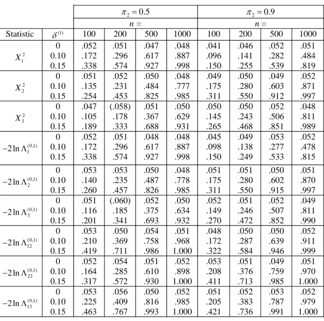
Table 3 summarizes the results for test of M(0) against M(1). From top to bottom there are three chi-square statistics and three MLR statistics based on transitions at the single times 1, 2 and 3. These are followed by two MLR statistics based on transitions at times (1, 2) and (2, 3). Finally, there is one MLR statistic based on transitions at the times (1, 2, 3).

Table 3. Simulated powers of various statistics for testing M(0) against M(1) at the 5 % significance level. δ(1)

is the difference between the parameters under M(0) and M(1). Two values of the null power that are suspiciously large are shown within parentheses.

2 0.5 π = π₂ =0.9 n = n = Statistic δ(1) _{100 200 500 1000 100 200 500 1000} 2 1 X 0 0.10 0.15 .052 .172 .338 .051 .296 .574 .047 .617 .927 .048 .887 .998 .041 .096 .150 .046 .141 .255 .052 .282 .539 .051 .484 .819 2 2 X 0 0.10 0.15 .051 .135 .254 .052 .231 .453 .050 .484 .825 .048 .777 .985 .049 .175 .311 .050 .280 .550 .049 .603 .912 .052 .871 .997 2 3 X 0 0.10 0.15 .047 .105 .189 (.058) .178 .333 .051 .367 .688 .050 .629 .931 .050 .145 .265 .050 .243 .468 .052 .506 .851 .048 .811 .989 (0,1) 1 2 ln − Λ 0 0.10 0.15 .052 .172 .338 .051 .296 .574 .048 .617 .927 .048 .887 .998 .045 .098 .150 .049 .138 .249 .053 .277 .533 .052 .478 .815 (0,1) 2 2 ln − Λ 0 0.10 0.15 .053 .140 .260 .053 .235 .457 .050 .487 .826 .048 .778 .985 .051 .175 .311 .051 .280 .550 .050 .602 .915 .051 .870 .997 (0,1) 3 2 ln − Λ 0 0.10 0.15 .051 .116 .201 (.060) .185 .341 .052 .375 .693 .050 .634 .932 .052 .149 .270 .051 .246 .472 .052 .507 .852 .049 .811 .990 (0,1) 12 2 ln − Λ 0 0.10 0.15 .053 .210 .419 .050 .369 .711 .054 .758 .986 .051 .968 1.000 .048 .172 .322 .050 .287 .584 .050 .639 .946 .052 .911 .999 (0,1) 23 2 ln − Λ 0 0.10 0.15 .052 .164 .317 .054 .285 .572 .051 .610 .930 .052 .898 1.000 .053 .208 .411 .051 .376 .713 .049 .759 .985 .051 .970 1.000 (0,1) 13 2 ln − Λ 0 0.10 0.15 .053 .225 .463 .056 .409 .767 .050 .816 .993 .052 .985 1.000 .051 .205 .421 .052 .383 .736 .053 .787 .991 .052 .979 1.000

When δ( )1 =0 the null power should be 0.050. However, in Table 3 there are two values of the null power that are too large in order to be accepted and these are given within

MLR statistic., although the latter seems to have slightly larger power. As expected, the non-null power increased with increasing n for given ( )1 ₂

andπ

δ .

One can note that that the powers behaved differently for π₂ =0.5andπ₂ =0.9. Consider e.g. the power of −2lnΛˆ(_t0,1) ,t=1,2,3, for a specific value of δ( )1 >0

. When π₂ =0.5the power steadily decreased with increasing t, but when π₂ =0.9the power was largest for t = 2. There is a simple explanation for this, namely that it can be shown that in the former case the expected working sample size, E

(

Nt(1)

)

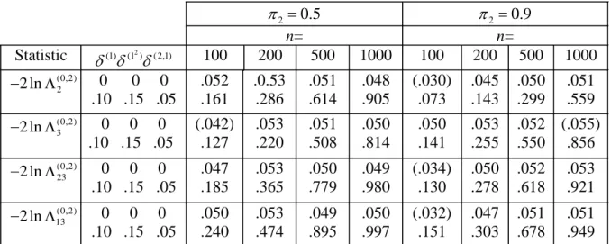
, is strictly decreasing with t, whereas in the latter case it has a maximum at t = 2. A further conclusion from Table 3 is that the power was increased if transitions from several time points were used.

The behavior of four power functions for testing M(0) against M(2) is illustrated in Table 4. Two powers are based on transitions from the separate time points 2 and 3, one power is based on transitions at (2,3) and one power from transitions at (1,2,3). The null power was close to 0.05 except when n = 100, in which case the null power sometimes was far below 0.05. This unwanted performance of the MLR test, with a local bias of the test, is well known (see e.g. [6]). But it is interesting that this pattern occurred more frequently with test of M(0) against M(2) than with test of M(0) against M(1). This raises the question whether tests of M(m) against M(m*) in general tend to be more biased as m* deviates from m.

Table 5 shows some values of the power function when testing M(1) against M(2). The case δ(1) ≠0 ,δ(12) =δ(2,1) =0corresponds to the situation under M(1). Also here there was a close agreement between the powers based on the statistics X_t(1,2) and−2lnΛˆ(_t1,2) ,t =2,3. As in Tables 3 and 4 the power was increased if data from more time points were used. (There was one exception from this when π₂ =0.9andn=100.) Comparing the non-null powers in Table 5 with those in Table 4 where test of the more deviating hypothesis M(0) against M(2) was considered, it is striking that the powers in Table 4 always dominated the powers in Table 5.

Table 4. Simulated powers of some statistics for testing M(0) against M(2) at the 5 % significance level. The δ -parameters express the differences between the parameters under H1 and H0 (see Section 4.1). Figures within parentheses show null powers that deviate too

much from the scheduled value 0.050.

2 0.5 π = π₂ =0.9 n= n= Statistic _{(1) (1 )}2 _(2,1) δ δ δ 100 200 500 1000 100 200 500 1000 (0,2) 2 2 ln − Λ 0 0 0 .10 .15 .05 .052 .161 .0.53 .286 .051 .614 .048 .905 (.030) .073 .045 .143 .050 .299 .051 .559 (0,2) 3 2 ln − Λ 0 0 0 .10 .15 .05 (.042) .127 .053 .220 .051 .508 .050 .814 .050 .141 .053 .255 .052 .550 (.055) .856 (0,2) 23 2 ln − Λ 0 0 0 .10 .15 .05 .047 .185 .053 .365 .050 .779 .049 .980 (.034) .130 .050 .278 .052 .618 .053 .921 (0,2) 13 2 ln − Λ 0 0 0 .10 .15 .05 .050 .240 .053 .474 .049 .895 .050 .997 (.032) .151 .047 .303 .051 .678 .051 .949

Table 5. Simulated powers of some statistics for testing M(1) against M(2) at the 5 % significance level. The δ -parameters and the figures within parentheses are interpreted as in Table 4. 2 0.5 π = π₂ =0.9 n = n = Statistic _{(1) (1 )}2 _(2,1) δ δ δ 100 200 500 1000 100 200 500 1000 2 2 X .10 .10 .10 .10 .15 .05 .10 .25 .05 .053 .109 .260 .049 .159 .470 .054 .324 .858 .051 .562 .988 (.021) .044 .082 (.043) .094 .215 .051 .162 .475 .050 .278 .764 2 3 X .10 .10 .10 .10 .15 .05 .10 .25 .05 .046 .067 .174 .052 .116 .326 .051 .227 .682 .049 .389 .928 .052 .090 .230 .048 .138 .401 .051 .275 .764 .052 .488 .968 (1,2) 2 2 ln − Λ .10 .10 .10 .10 .15 .05 .10 .25 .05 (.055) .113 .265 .050 .161 .473 .054 .326 .858 .051 .563 .988 (.024) .044 .084 .051 .095 .215 .054 .159 .472 .051 .272 .760 (1,2) 3 2 ln − Λ .10 .10 .10 .10 .15 .05 .10 .25 .05 .050 .075 .185 .054 .125 .333 .052 .228 .685 .050 .394 .929 .056 .094 .238 .049 .139 .405 .051 .275 .765 .053 .488 .968 (1,2) 23 2 ln − Λ .10 .10 .10 .10 .15 .05 .10 .25 .05 .054 .110 .314 .054 .183 .575 .052 .392 .947 .052 .677 .990 (.038) .075 .214 .049 .147 .445 .053 .298 .842 .052 .541 .990

5.5 Comparison between AIC and BIC

Table 6 summarizes the performance of the AIC and BIC procedures for estimating the Markov order m. For m = 0 it is evident that BIC performed better than AIC. The latter was not improved as n increased, thus showing the same inconsistency that was noticed in [10]. It is also peculiar that AIC placed Markov order 2 in front of Markov order 1. For m = 1 both procedures gave poor estimates unless n was 500 or larger. In this case, as well as for m = 2

Table 6. Comparison between the AIC and BIC procedures for estimating the Markov order m. The m-values to the left are those that were used in the simulations, while the six columns to the right show the relative frequencies (%) of the estimates of m.

ˆ_AIC m = mˆ_BIC = 2 0.5 π = n 0 1 2 0 1 2 0 m= 100 200 500 1000 81.6 78.1 78.9 78.6 7.8 7.5 7.5 7.7 10.6 14.4 13.6 13.7 97.4 97.4 98.7 99.2 2.4 2.4 1.2 0.8 0.2 0.2 0.1 0.0 1 m= 100 200 500 1000 56.1 40.3 13.1 1.6 33.2 47.1 71.8 82.6 10.7 12.6 15.1 15.8 75.8 68.2 42.5 14.2 21.5 29.6 55.7 84.4 2.7 2.2 1.8 1.4 2 m= 100 200 500 1000 13.2 0.9 0.0 0.0 4.0 0.4 0.0 0.0 82.8 98.7 100.0 100.0 34.0 8.0 0.0 0.0 5.0 0.8 0.0 0.0 61.0 91.2 100.0 100.0 2 0.9 π = n 0 1 2 0 1 2 0 m= 100 200 500 1000 77.6 78.7 78.2 78.4 8.2 7.1 7.9 7.9 14.2 14.2 13.9 13.7 96.6 97.4 98.6 99.3 2.8 2.3 1.2 0.7 0.6 0.3 0.2 0.0 1 m= 100 200 500 1000 47.2 28.4 5.2 0.2 41.2 58.5 79.1 84.0 11.7 13.1 15.8 15.8 70.3 56.5 24.0 3.6 26.9 41.0 74.0 95.1 2.8 2.5 2.0 1.3 2 m= 100 200 500 1000 24.2 5.0 0.0 0.0 14.2 5.4 0.1 0.0 61.6 89.6 99.9 100.0 49.6 24.0 1.0 0.0 14.4 10.3 1.2 0.0 36.0 65.7 97.8 100.0

AIC performed better.

As was mentioned in Section 3.3, the BIC criterion has been found to be superior to AIC in large samples for homogeneous MCs of order less than three. In the present study, where the parameter values varied in time, a somewhat different conclusion is reached.

5.6 Power of some tests of homogeneity

Tests of homogeneity for the case m = 1 can be based on the statistics in Section 4. Tests can be performed for one of the two type of parameters, or for both. The four parameter settings are described in Table 7, where the notation PS_tis used for a set of parameter values that gradually increase from 0.60 to 0.60+0.05(t-1), t =2,…,7.

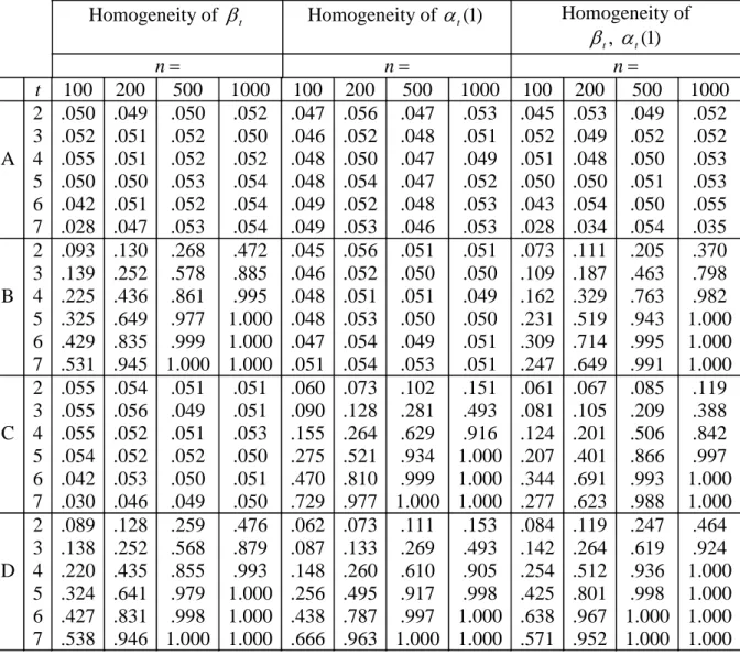
Table 7. Summary of some desired properties of the power when performing various tests of homogeneity in the parameter settings (A)-(D).

Homogeneity of t β α_t(1) β α_t, (1)_t (A) β α_t = _t(1)=0.60 .05 .05 .05 Parameter (B)βt∈PSt, (1)αt =0.60 >.05 .05 >.05 Setting (C)β_t =0.60, (1)α_t ∈PS_t .05 >.05 >.05 (D)β_t∈PS_t, (1)α_t ∈PS_t >.05 >.05 >.05

The results from the simulations are given in Table 8. It is seen that the null-power behaved as desired, possibly with a few exceptions when n≤200or t≥6. In the latter case the random sample sizes Nt(1)andNt(2)were too small for the chi-square approximation to hold, and sometimes even zero. On the whole the non-null power increased with n and also with t. The largest power was obtained when homogeneity of both β_t andα_t(1)was tested and there was a true shift in both parameters.

Table 8. Values of the power when testing for homogeneity in the four parameter settings (A)-(D) given in Table 7.

Homogeneity of β_t Homogeneity of α_t(1) Homogeneity of , (1) t t β α n= n= n= t 100 200 500 1000 100 200 500 1000 100 200 500 1000 A 2 3 4 5 6 7 .050 .052 .055 .050 .042 .028 .049 .051 .051 .050 .051 .047 .050 .052 .052 .053 .052 .053 .052 .050 .052 .054 .054 .054 .047 .046 .048 .048 .049 .049 .056 .052 .050 .054 .052 .053 .047 .048 .047 .047 .048 .046 .053 .051 .049 .052 .053 .053 .045 .052 .051 .050 .043 .028 .053 .049 .048 .050 .054 .034 .049 .052 .050 .051 .050 .054 .052 .052 .053 .053 .055 .035 B 2 3 4 5 6 7 .093 .139 .225 .325 .429 .531 .130 .252 .436 .649 .835 .945 .268 .578 .861 .977 .999 1.000 .472 .885 .995 1.000 1.000 1.000 .045 .046 .048 .048 .047 .051 .056 .052 .051 .053 .054 .054 .051 .050 .051 .050 .049 .053 .051 .050 .049 .050 .051 .051 .073 .109 .162 .231 .309 .247 .111 .187 .329 .519 .714 .649 .205 .463 .763 .943 .995 .991 .370 .798 .982 1.000 1.000 1.000 C 2 3 4 5 6 7 .055 .055 .055 .054 .042 .030 .054 .056 .052 .052 .053 .046 .051 .049 .051 .052 .050 .049 .051 .051 .053 .050 .051 .050 .060 .090 .155 .275 .470 .729 .073 .128 .264 .521 .810 .977 .102 .281 .629 .934 .999 1.000 .151 .493 .916 1.000 1.000 1.000 .061 .081 .124 .207 .344 .277 .067 .105 .201 .401 .691 .623 .085 .209 .506 .866 .993 .988 .119 .388 .842 .997 1.000 1.000 D 2 3 4 5 6 7 .089 .138 .220 .324 .427 .538 .128 .252 .435 .641 .831 .946 .259 .568 .855 .979 .998 1.000 .476 .879 .993 1.000 1.000 1.000 .062 .087 .148 .256 .438 .666 .073 .133 .260 .495 .787 .963 .111 .269 .610 .917 .997 1.000 .153 .493 .905 .998 1.000 1.000 .084 .142 .254 .425 .638 .571 .119 .264 .512 .801 .967 .952 .247 .619 .936 .998 1.000 1.000 .464 .924 1.000 1.000 1.000 1.000

6. An application: Test of Markov order and homogeneity in rehabilitation data 6.1 Markov order

In a Swedish study 2440 sick-listed women and 1801 sick-listed men were followed after start of a rehabilitation period. At the beginning of each quarter t = 1,…,8 each person was classified into one of the states 0 (Healthy), 1 (Improved) and 2 (Acute diseased) and initially

all persons were in state 1 or 2. The classification into the states was made by social insurance authorities. Results from the study, including further details about data, estimated transition probabilities and prediction probabilities, have been reported earlier [9]. In this paper focus will be on tests.

A first step in the analysis was to get knowledge about the dependency structure. Tables 9a and 9b show values of the chi-square statistics χ_t2 and theMLRstatistic−2lnΛˆ(_tm,m+1for testing M(m) against M(m+1), m = 0,1,2. Both statistics have an asymptotic chi-square distribution with 1 degree of freedom under the null hypothesis M(m). Since the 95 % percentile in the latter distribution is 3.84 the Markov orders 0 and 1 were rejected in most cases, but not Markov order 2. Two exceptions from this were obtained for the MLR test at quarter 6 for women and quarter 7 for men. But here one has to take into consideration that the working sample sizes were very small, e.g. N_t(2,1)was far below 20 for both sexes. When testing M(1) against M(2) for a sequence of transitions from quarter 2 to quarter 6 the MLR statistic for women was 44, to be compared with 11.07 which is the 95 % percentile of the chi-square distribution on 5 ( 6-2+1) degrees of freedom. So Markov order 1 is strongly rejected. On the other hand, when M(2) was tested against M(3) the MLR statistic was 3.7 which is far below the rejection limit 9.45 (df = 6-3+1) so there was no reason to reject a Markov order of 2. Similar results were obtained for men.

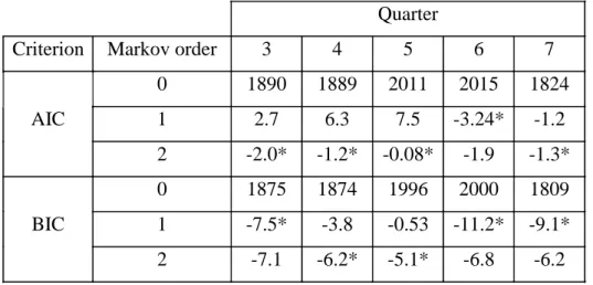
The use of AIC and BIC criteria for estimating Markov order gave a somewhat unclear picture, as is seen in Table 10. In most cases a Markov order of 2 is suggested. But there are exceptions at the quarters 6 and 7 where a Markov order of 1 is suggested in a similar way as was seen in Table 9b. The total AICs computed from all quarters were for women 9629 (m = 0), 18 (m = 1), -6.3 (m = 2) and for men 5855 (m = 0), 58 (m = 1), -4.8 (m = 2), thus suggesting that m = 2.

Table 9a. Chi-square statistics for tests of Markov order. Quarter

Sex Markov order 1 2 3 4 5 6 7

M(0) vs M(1) 1134 1406 1581 1559 1612 1609 1497 Women M(1) vs M(2) - 11.4 8.6 14.9 21.3 4.3 8.1 M(2) vs M(3) - - 0.19 0.95 0.99 0.17 0.39 M(0) vs M(1) 707 816 928 938 955 995 956 Men M(1) vs M(2) - 21.7 27.5 12.6 29.2 55.0 4.6 M(2) vs M(3) - - 0.20 0.01 1.93 0.30 0.29

Table 9b. MLR statistics for tests of Markov order.

Quarter

Sex Markov order 1 2 3 4 5 6 7

M(0) vs M(1) 1236 1609 1890 1885 2003 2018 1825 Women M(1) vs M(2) - 10.1 6.7 9.4 11.5 2.6 4.0 M(2) vs M(3) - - 0.02 0.84 1.9 0.15 0.76 M(0) vs M(1) 766 920 1082 1134 1167 1241 1184 Men M(1) vs M(2) - 19.1 20.9 9.7 16.2 23.3 2.8 M(2) vs M(3) - - 2.5 0.01 1.6 0.58 0.56 6.2 Homogeneity

In a non-homogeneous MC of order 2 there are three transition probabilities to estimate at each t≥2, , (12)and (2,1)

t t

t α α

β . Plots of the latter against t were presented in Figure 2 in [9], where it is apparent that the transition probabilities are non-stationary at earlier quarters. Table 11 summarizes the results from tests of homogeneity by means of the MLR statistics suggested in Section 4. Test of stationarity of αt(2,1)was not performed due to very small working sample sizes. The results in Table 11 agree very well with the pattern that was noticed in the plots, i.e. a non-homogeneous pattern at early quarters that later turns into a

Table 10. Estimation of Markov order by means of the AIC and BIC criteria, (a) for women and (b) for men. The smallest values of the AIC- and BIC statistics at each quarter are marked by an asterisk.

(a)

Quarter

Criterion Markov order 3 4 5 6 7 0 1890 1889 2011 2015 1824 AIC 1 2.7 6.3 7.5 -3.24* -1.2 2 -2.0* -1.2* -0.08* -1.9 -1.3* 0 1875 1874 1996 2000 1809 BIC 1 -7.5* -3.8 -0.53 -11.2* -9.1* 2 -7.1 -6.2* -5.1* -6.8 -6.2 (b) Quarter

Criterion Markov order 3 4 5 6 7 0 1099 1138 1178 1259 1181 AIC 1 19.4 5.7 11.8 17.9 -2.7* 2 0.52* -1.9* -0.42* -1.4* -1.4 0 1085 1124 1165 1246 1168 BIC 1 10.1 -3.4 4.9 11.1 -9.4* 2 -4.1* -6.6* -4.9* -5.8* -5.8

homogeneous pattern. In Table 11 one may notice that it is easier to reject homogeneity during longer periods. E.g. in Table 11 (a) for women, homogeneity was not rejected at transitions from 3 to 4, from 4 to 5 and from 5 to 6, but homogeneity was strongly rejected if transitions from 2 to 6 were considered.

Table 11. MLR statistics for testing homogeneity from quarter u to quarter v among men and women, (a) for β_t and (b) for 2

(1 ) t

α . Values within parentheses indicate non-significance at the 5 % level.

(a) Women Men v v 2 3 4 5 6 7 2 3 4 5 6 7 1 53 121 171 231 279 283 15 36 83 115 140 145 2 11 18 35 47 50 (3.5) 24 36 45 45 u 3 (.32) 5.7 9.3 20 9.6 13 15 17 4 (3.1) (4.7) 18 (.01) (.01) (5.1) 5 (.03) 18 (.01) (4.4) 6 13 (3.4) (b) Women Men v v 3 4 5 6 7 3 4 5 6 7 2 9.8 18 37 57 78 10 12 24 63 99 u 3 (.70) 8.5 17 28 (.35) (5.2) 31 53 4 4.1 8.7 14 4.9 27 44 5 (.66) (2.3) 8.9 15 6 (.48) (.59) 7. Conclusions

In [9] it was demonstrated that a correct specification of Markov order and homogeneity is highly important. It is therefore interesting to study to which degree it is possible to make correct specifications based on tests. In Section 6 one statistic based on the chi-square criterion and one based on the MLR criterion was evaluated when testing for Markov order m. Also the use of AIC and BIC was studied for obtaining an estimate of m. From Tables 3 and 5 it is concluded that a sample size (n) of at least 500, or even 1000, is needed in order to reach an acceptable level of the power. The procedures based on AIC and BIC also require large sample sizes in order to be reliable. However, even with n = 1000 AIC works less well when

estimating Markov orders less than 2. The difference in power between the two statistics for test of Markov order was small, possibly with a slight advantage for the MLR statistic.

When testing for homogeneity the largest power was obtained when (i) a long period of transitions was used and (ii) homogeneity of several different parameters were considered simultaneously, and there actually was a shift in all of them. In the application (Section 6) it was found that homogeneity was rejected when the test was based on a long period of transitions, but not when the test was based on a single transition mostly towards the end of the studied period. The latter might be explained by the fact that there actually was a stabilization of the parameters towards the end, but this could not be detected by a ‘long-period test’.

In conclusion, it is recommended to use all procedures that were considered in Sections 3 and 4 in the same way as was done in Section 6. One should also be aware of the fact that failure of rejecting a hypothesis may be due to a small working sample size, even if the fixed total sample size (n) is large.

Acknowledgements

The research was supported by the National Social Insurance Board in Sweden (RFV), Dnr 3124/99-UFU.

References

1. Akaike, H., “A new look at the statistical model identification”, IEEE Transactions on Automatic Control 19, 716-723, 1974.

2. Avery, P.J. and Henderson, D.A., “Fitting Markov chain models to discrete state series such as DNA sequences”, Applied Statistics 48, 53-61, 1999.

3. Diebold, F.X., Lee, J-H. and Weinbach, G.C., “Regime switching with time-varying probabilities”, in Nonstationary Time Series Analysis and Cointegration (Hargreaves, C. ed.), 283-302, Oxford University Press, Oxford, 1994.

4. Gabriel, K. and Neumann, J., “A Markov chain model for daily rainfall occurrence at Tel Aviv”, Quarterly Journal of the Royal Meteorological Society 88, 90-95, 1962.

5. Gates, P. and Tong, H., “On Markov chain modeling to some weather data”, Journal of Applied Meteorology 15, 1145-1151, 1976.

6. Hayakawa, T., “The likelihood ratio criterion for composite hypothesis under a local alternative”, Biometrika 62, 451-460, 1975.

7. Hoel, P.G., “A test for Markoff chains”, Biometrika 41, 430-433, 1954.

8. Hughes, J.P., Guttorp, P. and Charles, S.P., “A non-homogeneous hidden Markov model for precipitation occurrence”, Applied Statistics 48, 15-30, 1999.

9. Jonsson, R., “A Markov chain model for analyzing the progression of patient’s health state”, Research Report 2011:6, Statistical Research Unit, Göteborg University, Sweden, 2011.

10.Katz, R.W., “On some criteria for estimating order of a Markov chain”, Technometrics

23, 243-249, 1981.

11.Lowry, W.P. and Guthrie, D., “Markov chains of order greater than one”, Monthly Weather Review 96, 798-801, 1968.

12.Schwartz, G., “Estimating the dimension of a model”, Annals of Statistics 6, 461-464, 1999.

13.Stuart, A., Ord, J.K. and Arnold, S., Kendalls Advanced Theory of Statistics Vol. 2A, Arnold, London, 1999.

14.Van den Berg, G., in Specification, Identification and Multiple Duration (Heckman, J. and Leaner, E. eds.), Handbook of Econometrics, Vol. V, North Holland, Amsterdam, 2001.

Appendix

A1. The Likelihood of the three-state Markov chain of order m The likelihood ( )m

L of all observations in the three-state model of Markov order m can be expressed as 1 (2) ( ) ( ) ( ) 1 (1 ) t t t T B N B m m m t t t L C β β F G − − = = ⋅

∏

− ⋅ ⋅

Here C is a constant that does not depend on the α- and β-parameters, and

[

] [

]

1 (1) (1) (1) 1 ( ) 1 _{(1 ) (1 ) (1 )} 1 _{(1 ) (1 ) (1 )} 1 (1) 1 (1) , if 1 (1 ) 1 (1 ) (1 ) 1 (1 ) , if 2 t t t t t t m m m t t t t t t T A N A t t t m m _{A N A} T _{A N A} t t m m t t t t t t m m F m α α α α α α − ₋ = − ₋ − ₋ = =  _{− =}  =     −     −  ≥        

∏

∏

∏

   1 1 1 ( ) ₁ (2,1 ) (2,1 ) (2,1 ) 1 1 2 1, if 1 (2,1 ) 1 (2,1 ) , if 2 i i i t t t m _{m T} A N A i i t t i t i m G m α − α − − − ₋ − − = = =   =  _{   −  ≥}      

∏∏

A proof of the above expression is outlined in the Appendix A1 in [9].

A2. The MLR statistic for testing M(m) against M(m*), 0<m<m*

By the same arguments that were used in Section 3.1 it follows that the MLR statistic is

∏

− = − −       − −             − −       = Λ 1 * (2,1) (2,1) (2,1) ) 1 ( ) 1 ( * ) 1 ( * ) , ( ) 1 , 2 ( ˆ 1 ) 1 ( ˆ 1 ) 1 , 2 ( ˆ ) 1 ( ˆ ) 1 ( ˆ 1 ) 1 ( ˆ 1 ) 1 ( ˆ ) 1 ( ˆ ˆ * * * * m m s A N s i m i A s i m i A N m i m i A m i m i m m i s i s i s i m i m i m i α α α α α α α α

Under the hypothesis of M(m), −2lnΛˆ(_im,m*)has a chi-square distribution with df = m* - m. When the same hypothesis is tested for a sequence of transitions from s≥m+1 tot ≤T −1, the MLR statistic is

∏

= Λ = Λ t s i m m i m m t s *) , ( *) , ( , ˆ ˆ _where ( , *) , ˆ ln 2 Λ_sm_tm

− is chi-square distributed with df = (m* -m)(t – s +1).

A3. Proof of the relations leading to the test statistic in (13a)

In Section 3.2 it was stated that two differences between estimators can be expressed in terms of one common difference. The ML estimator of α_t(1m)is

) 1 , 2 ( ) 1 ( ) 1 , 2 ( ) 1 , 2 ( ˆ ) 1 ( ) 1 ( ˆ ) 1 , 2 ( ) 1 ( ) 1 , 2 ( ) 1 ( ) 1 ( ) 1 ( 1 1 1 1 1 m t m t m t m t m t m t m t m t m t m t m t m t N N N N N N A A N A + ⋅ + ⋅ = + + = ₊+ α + +₊ α .

From this it follows that

[

]

) 1 ( ) 1 , 2 ( ) 1 , 2 ( ˆ ) 1 ( ˆ ) 1 ( ˆ ) 1 ( ˆ 1 1 m t m t m t m t m t m t N N ⋅ − = − + + _{α α α} α

Similarly one obtains

[

]

) 1 ( ) 1 ( ) 1 ( ˆ ) 1 , 2 ( ˆ ) 1 ( ˆ ) 1 , 2 ( ˆ 1 1 m t m t m t m t m t m t N N + + _⋅ − = −α α α α .

Research Report

2007:1 Andersson, E.: Effect of dependency in systems for multivariate surveillance.

2007:2 Frisén, M.: Optimal Sequential Surveillance for Finance, Public Health and other areas.

2007:3 Bock, D.: Consequences of using the probability of a false alarm as the false alarm measure.

2007:4 Frisén, M.: Principles for Multivariate Surveillance.

2007:5 Andersson, E., Bock,

D. & Frisén, M.: Modeling influenza incidence for the purpose of on-line monitoring. 2007:6 Bock, D., Andersson,

E. & Frisén, M.: Statistical Surveillance of Epidemics: Peak Detection of Influenza in Sweden. 2007:7 Andersson, E.,

Kuhlmann, S., Linde., A &Frisén, M.:

Predictions by early indicators of the progress of the influenza in Sweden.

2007:8 Bock, D., Andersson,

E. & Frisén, M.: Similarities and differences between statistical surveillance and certain decision rules in finance.

2007:9 Bock, D.: Evaluations of likelihood based surveillance of

volatility. 2007:10 Bock, D. & Pettersson,

K.: Explorative analysis of spatial aspects on the Swedish influenza data. 2007:11 Frisén, M. &

Andersson, E.: On-line detection of outbreaks. 2007:12 Frisén, M., Andersson,

E. & Schiöler, L.: A non-parametric system for on-line outbreak detection of epidemics. 2007:13 Frisén, M., Andersson,

E. & Pettersson, K.: Estimation of outbreak regression.

2007:14 Pettersson, K.: Unimodal regression in the two-parameter exponential family with constant dispersion parameter.

2008:1 Frisén, M. Introduction to financial surveillance. 2008:2

2008:3

Jonsson, R. Andersson, E.

When does Heckman’s two-step procedure for censored data work and when does it not? Hotelling´s T2 Method in Multivariate On-Line Surveillance. On the Delay of an Alarm.

2008:4 Schiöler, L. & Frisén, M. On statistical surveillance of the performance of fund managers.

2008:5 Schiöler, L. Explorative analysis of spatial patterns of influenza incidences in Sweden 1999—2008.

2008:6 Schiöler, L. Aspects of Surveillance of Outbreaks.

2008:7 Andersson, E & Frisén, M.

Statistiska varningssystem för hälsorisker 2009:1 Frisén, M., Andersson, E.

& Schiöler, L.

Evaluation of Multivariate Surveillance 2009:2 Frisén, M., Andersson, E.

& Schiöler, L.

Sufficient Reduction in Multivariate Surveillance

2010:1 Schiöler, L Modelling the spatial patterns of influenza

incidence in Sweden

2010:2 Schiöler, L. & Frisén, M. Multivariate outbreak detection

2010:3 Jonsson, R. Relative Efficiency of a Quantile Method for

Estimating Parameters in Censored Two-Parameter Weibull Distributions

2010:4 Jonsson, R. A CUSUM procedure for detection of outbreaks

in Poisson distributed medical health events

2011:1 Jonsson, R. Simple conservative confidence intervals for

comparing matched proportions

2011:2 Frisén, M On multivariate control charts

2011:3 2011:4 2011:5 2011:6 Frisén, M Knoth, S &Frisén, M Marianne Frisén Robert Jonsson

Methods and evaluations for surveillance in industry, business, finance, and public health Minimax Optimality of CUSUM for an

Autoregressive Model

Inference principles for multivariate surveillance  A Markov Chain Model for Analysing the