University of Richmond
UR Scholarship Repository
Math and Computer Science Faculty Publications
Math and Computer Science
2016
On Data Depth and the Application of
Nonparametric Multivariate Statistical Process
Control Charts
Suk Joo Bae
Giang Do
Paul Kvam
University of Richmond, [email protected]
Follow this and additional works at:
http://scholarship.richmond.edu/mathcs-faculty-publications
This is a pre-publication author manuscript of the final, published article.
This Post-print Article is brought to you for free and open access by the Math and Computer Science at UR Scholarship Repository. It has been accepted for inclusion in Math and Computer Science Faculty Publications by an authorized administrator of UR Scholarship Repository. For more information, please [email protected].
Recommended Citation
Bae, Suk Joo; Do, Giang; and Kvam, Paul, "On Data Depth and the Application of Nonparametric Multivariate Statistical Process Control Charts" (2016).Math and Computer Science Faculty Publications. 168.
On Data Depth and the Application of Nonparametric
Multivariate Statistical Process Control Charts
Suk Joo Bae ∗, Giang Do†, Paul Kvam‡
Abstract
The purpose of this article is to summarize recent research results for constructing nonparametric multivariate control charts with main focus on data depth based control charts. Data depth provides data reduction to large-variable problems in a completely nonparametric way. Several depth measures including Tukey depth are shown to be particularly effective for purposes of statistical process control in case that the data deviates normality assumption. For detecting slow or moderate shifts in the process target mean, the multivariate version of the EWMA is generally robust to non-normal data, so that nonparametric alternatives may be less often required.
Keywords: Data depth, HotellingT2statistic, Mahalanobis distance, Shewhart chart, Tukey
depth.
1
Introduction
A control chart is a traditional way of monitoring the sequential stability of a single variable in a process under parametric assumption. In modern statistical process control (SPC), a large number of quality characteristics are becoming accessible through on-line computers and other advanced data-acquisition equipments. There is a well recognized need for mul-tivariate methods to handle complex applications that monitor a large number of variables simultaneously. By now, there has been a substantial body of research addressing problem issues for multivariate data in SPC. Despite this recent surge in new charts for multivariate
∗Suk Joo Bae is Associate Professor in Department of Industrial Engineering, Hanyang University, Seoul,
Korea ([email protected])
†Giang Do is Ph.D. candidate in the School of Mathematics, Georgia Institute of Technology, Atlanta,
GA, USA 30332 ([email protected])
‡P. Kvam is Professor in the School of Industrial & Systems Engineering, Georgia Institute of Technology,
data, they are not highly appreciated by managers who use control charts to identify and eliminate assignable causes of variation from a process.
There are two formidable challenges in analyzing multivariate process data. First, data become more sparse as dimensions increase. Sample size requirements are formidable - a reference sample of hundreds to thousands of observations can be needed to fully characterize an in-control process if three or more quality variables are being measured. Another big problem is that the control charting methods become more dependent on the assumption that the input measurements are normally distributed, while at the same time, the normality assumption becomes less plausible in multivariate settings. If multivariate control charts are to find a place in statistical practice, they need to address problems with correlated non-normal data. If traditional (parametric) methods are not found to be robust, we need to focus instead on nonparametric multivariate control charting techniques.
With these serious impediments, practitioners have continued to rely on univariate con-trol charting techniques by treating individual variables independently for multivariate data. Multivariate methods are not highly emphasized in non-technical books. In Montgomery’s popular Introduction to Statistical Process Control(2005), simultaneous monitoring is suc-cinctly reviewed, yet relegated to a late chapter, which suggests that multivariate methods are not part of the core study for a quality control class. Recognizing the need of multivari-ate methods in SPC, Alt and Smith (1988) and Lowry and Montgomery (1995) reviewed control charts for multivariate normal data since the mid-1980s. Recently, multivariate methods for process control are getting more attention in industry to monitor the stabil-ity of certain sequential processes. Yeh et al. (2006) and Bersimis et al. (2007) surveyed parametric multivariate chart techniques based mainly on multivariate normal processes, providing a helpful discussion for practitioners about how to implement and interpret mul-tivariate methods.
In this article, we will go over the current state ofnonparametric methodsin multivariate process control. To complement this study, there are several overviews of nonparametric methods used in SPC, including a comprehensive survey of rank-based extensions for tra-ditional (univariate) control charts in Chakraborti et al. (2001). It is important to note, however, that there is virtually no intersection between these review articles. That is, prac-titioners seeking information about nonparametric multivariate control charts will not find the topic covered in either review.
In Sections 2 and 3, we will review the literature comprising the two separate branches of multivariate statistical process control and nonparametric control charting. In Sections 4, we will review the literature on nonparametric multivariate control charts. In Section 5, we
will focus on the only well-known nonparametric multivariate control charting techniques based on the concept of data depth. Data depth techniques for dimension reduction are based on measuring how “outlying” a given multivariate observation (or entire sample) is with respect to an underlying population or distribution.
We feature two general categories of control charts that solve two different process control problems. Shewhart-type charts (e.g., ¯x-R chart,p-chart) use information from the most current sample in order to detect a sudden change in the process mean. Shewhart charts are useful for detecting change-points in the process target mean unless the mean shift is gradual and cannot be detected in a single sample. As an alternative, accumulative-type charts such as the cumulative sum (CUSUM) chart or the exponentially weighted moving average (EWMA) chart are constructed to detect slow and moderate shifts in the mean that occur across sequential samples. These two types of charts serve different purposes for the process manager, and they also have different performance issues when we try to extend them to include nonparametric applications.
2
Multivariate control charts
Before multivariate process control techniques were used in practice, it was common to monitor multiple variables by ignoring the multivariate distribution of the input data and creating separate charts for individual variables. This approach can lead to grossly incorrect control limits, especially when the monitored data are correlated. Even if the inputs are uncorrelated, individual monitoring has to be calibrated in order to understand the (type I) error rates that are associated with deciding that an in-control process is out of control. For example, if two quality characteristics are monitored using 3σcontrol limits, the probability either variable exceeds the control limits is P(|Z| > 3) = 0.0027, where Z ∼ N(0,1). But the probability both variables are simultaneously within control limits is reduced to 0.99732 = 0.9946, so the type I error rate is nearly doubled to 0.0054. As the number of monitored variables increases tok, the type I error for the process goes from the individual error levelα to 1−(1−α)k.
For Shewhart-type charts, the standard approach for analyzing multivariate process data is based on the Hotelling’s T2 statistic which is a natural multivariate extension to the univariate Shewart chart. The idea is based on the statistic n(¯x−µ)TΣ−1(¯x−µ), where ¯xis the sample mean from a multivariateNp(µ,Σ) (normal) distribution. There are
two distinct phases of control chart practice; Phase I consists of using the control charts for retrospectively testing whether the process was in control when the first m subgroups were drawn. The objective is to secure an in-control set of data to construct control limits
for future monitoring purposes. These control limits are used in Phase II to test whether the process remains in control when future subgroups are drawn at the second phase. Alt (1984) and Jackson (1985) discussed the methods for constructing the control limits for both phases of a multivariate process. For the Hotelling’sT2 chart, suppose that we sample
msubgroups of which sample sizes are larger than 1 in Phase I and compute (p×1) vectors of the sample means ¯x1,· · ·,x¯m, and (p×p) matrix of sample variances S1,· · ·,Sm for
each subgroup. Ifµand Σare unknown, µandΣare estimated by ¯x¯ and ¯S, respectively, then
Ti2=n(¯xi−x¯¯)TS¯−1(¯xi−x¯¯) (1)
has the Hotelling’s T2 distribution for the ith rational subgroup, where ¯x¯ is the overall mean and ¯S = (∑mj=1Sj)/m is the pooled sample variance-covariance matrix from the m
subgroups. The Hotelling’s T2 chart for the process mean, with unknown parameters, has the following upper control limit (UCL)
UCL = p(m+ 1)(n−1)
mn−m−p+ 1Fα,p,mn−m−p+1, (2) for the sample size n of the subgroup. The UCL is used to monitor future subgroups in Phase II. If the underlying input data is from the multivariate normal distribution, then the T2 statistic is appropriate, and the multivariate problem can be conveniently reduced to a single-variable test. Along with the normality assumption, Hotelling’sT2 control chart relies on the covariance structure remaining constant in time. Tracy et al. (1992) showed that the control limits for the Hotelling’sT2 statistic are not appropriate and follow a beta distribution if individual observation (n = 1) is used. Nedumaran and Pignatiello (1999) studied the effects of parameter estimation on multivariateT2 charts withχ2-based control limits. Champ et al. (2005) studied theT2 chart with corrected control limits based on the F distribution and showed that both the in-control and out-of-control average run lengths (ARLs) in the unknown parameter case are higher than ARLs in the known parameter case when estimating the parameters in the T2 statistic. For Shewhart-type charts, however, there are no straightforward extensions to common control charts that can be effectively applied to non-normal data.
Hotelling’s T2 chart, which is based only on the most recent observations, is insensi-tive to small and moderate shifts in process mean. For detecting slow or moderate shifts in the process mean, we can use a multivariate version of the CUSUM or another exten-sion based on the exponentially weighted moving average (MEWMA). Woodall and Ncube (1985) proposed the use of p univariate CUSUM charts for the p original variables or for
p principal components in p-dimensional multivariate normal process. This multiple uni-variate CUSUM scheme (called the MCUSUM) gives an out-of-control signal whenever any
of the univariate CUSUM charts is out of control. The MCUSUM scheme was applied to control process dispersion by Healy (1987) and to detect process mean shift for regression-adjusted variables by Hawkins (1991, 1993). Hauck et al. (1999) applied the MCUSUM chart to the multivariate process monitoring and diagnosis with grouped regression-adjusted variables. For modified versions of the MCUSUM chart, see Crosier (1988) and Pignatiello and Runger (1990). Ngai and Zhang (2001) provided a natural multivariate extension to the two-sided cumulative sum chart for controlling the process mean. Runger and Testik (2004) provided a comprehensive description and analysis of several multivariate exten-sions to CUSUM control charts, as well as performance evaluations and a description of their inter-relationships. The MCUSUM schemes have been employed in biomedical area, as well as industries. Rogerson and Yamada (2004) compared univariate and multivariate cumulative sum approaches for monitoring the change in spatial patterns of breast cancer in the northeastern United States. They observed that the univariate CUSUM scheme is generally better at detecting the changes in rates occurring in a small number of regions when the degree of spatial autocorrelation is low, while the multivariate CUSUM scheme is better at detecting the changes in rates occurring in a large number of regions. Noorossana and Baghefi (2006) investigated the performance of the MCUSUM chart in the presence of autocorrelation and suggested to use a time series model to improve the ARL properties of the MCUSUM control charts.
As a natural extension to the univariate EWMA chart, the MEWMA chart was proposed by Lowry et al. (1992) as follows
zi =Rxi+ (I−R)zi−1, i= 1,2,3, . . . (3)
where z0 = 0, R = diag(r1, r2, . . . , rp),0 ≤ rj ≤ 1 for j = 1, . . . , p, and I is the identity
matrix. The MEWMA chart gives an out-of-control signal if zTi Σ−z1zi > h, where Σz is the variance-covariance matrix of zi. The value h is calculated by simulation to achieve a
specific in-control ARL. Analogous to the situation in the univariate case, the MEWMA chart is equivalent to the Hotelling’s T2 chart if R = I. Lowry et al. (1992) showed that the ARL performance of the MEWMA chart is similar to that of the MCUSUM chart in detecting a shift in the mean of a multivariate normal distribution. For calculating in-control or out-of control ARL of the MEWMA chart, many ideas have been suggested, e.g., Rigdon (1995a, 1995b), Runger and Prabhu (1996), Bodden and Rigdon (1999), and Molnau et al. (2001). Stoumbos and Sullivan (2002) showed that the MEWMA scheme is fairly robust to non-normal data and very effective at detecting slow and subtle shifts even for highly skewed and heavy-tailed multivariate distributions. Testik et al. (2003) discussed robustness properties of MEWMA charts for multivariatetand multivariate gamma distributed data.
In designing the MEWMA charts, there are three different approaches: (1) statistical design; (2) economic-statistical design; and (3) robust design. A comparison of these three design strategies is provided by Testik and Borror (2004). Liu et al. (2004) studied a data depth-based moving average (DDMA) control chart to simultaneously detect location and scale changes of the process in the nonparametric setting. Yeh et al. (2004) proposed a likelihood-ratio-based EWMA control chart for detecting small changes in the process variability of multivariate normal processes. Lee and Khoo (2006) investigated the performance of the MEWMA control chart in ARL and median run length (MRL).
If a process is judged to be out of control, there are various ways of dissecting the process to find out which of the monitored inputs is responsible for the alarm. But this is a difficult problem to sort out. We can resort to gleaning univariate charts under the assumption that only one or two individual variables are responsible for the alarm. However, the signal of a multivariate chart can be due to a combination of several factors having to do not only with a drift from individual process means, but possibly from a detected difference in the correlation structure. Dimension reduction is then considered for multivariate charts in which the number of variables p is large and the use of traditional multivariate Shewhart charts or MCUSUM and MEWMA charts are less plausible. A common procedure for reducing the dimensionality of the variable space is to use projection methods such as principal component analysis (PCA) and partial least squares (PLS). The PCA reduces (p×p) non-singular sample covariance matrixSto a diagonal matrixLsuch thatUTSU=
L, where U is an orthonormal matrix. The diagonal elements of L,l1 ≥l2 ≥ · · · ≥ lp are
eigenvalues of S and the columns of U are the eigenvectors ofS. For (p×1) observations of original variables,x,ith principal componentzi =uTi (x−x¯) has mean zero and variance li, where ui is a normalized eigenvector such that uTi ui = 1. In general, because the first k(k < p) principal components explain the majority of process variance, they can be used for inference purposes to reduce the dimensionality of process variables. Runger and Alt (1996) proposed a method about how to choose k for process control purposes. Jackson (1991) presented three types of principal components control charts: (1) T2 chart based on principal components scores; (2) a principal components residual control chart; and (3) a control chart for each independent principal components scores. Ku et al. (1995) and Mastrangelo et al. (1996) extended the PCA models to autocorrelated data in process monitoring. The PCA methods were applied to analyze a historical set of batch trajectory data in multi-way form, e.g., Nomikos and MacGregor (1995a), Wise et al. (2001), and Cho and Kim (2003), to name a few.
in the process variables (X), but the variation in X which is most predictive of the quality variables (Y). The PLS accomplishes this by working on the sample covariance matrix (XTY)(YTX). MacGregor et al. (1994), Nomikos and MacGregor (1995b), and Kourti et. al. (1995) presented the use of PLS in multivariate SPC. Wang et al. (2003) proposed a recursive PLS modeling technique in the multivariate SPC framework. The applications of PLS, multi-way PLS, PCA, and multi-way PCA, or their modifications in real or simulation processes have been discussed by Martin and Morris (1996) and Simoglou et al. (2000). Kourti (2005) gave an overview of multivariate monitoring based on latent variable methods for detection and isolation of faults in industrial processes. Besides, Lee et al. (2004) proposed the use of independent component analysis (ICA) which decomposes observed data into linear combinations of statistically independent components to capture the essential structure of the data in the process. Wang and Tsung (2009) developed adaptive dimension reduction schemes to maintain the sampling distribution properties of the test statistic. This procedure can be effective on a limited number of multivariate SPC problems. Zou and Qiu (2009) developed a multivariate EWMA chart into which integrates a LASSO-based multivariate test statistic for phase II multivariate process monitoring.
3
Nonparametric control charts
Even with univariate control charts, the normality assumption has been a critical barrier in validating the statistical method with the process data. As mentioned in Kvam and Vidakovic (2007), simple control charts based on the assumptions of normality are not more useful because they are perfectly appropriate, rather because they are perfectly convenient. In some cases we can transform the data, and by choosing the right chart, such as the EWMA or CUSUM, the performance of these assumption-driven control charts can be respectable – see, for example, Borror et al. (1999).
Shewhart (1939) first considered the effect of non-normality on a control chart, specifi-cally the ¯x chart. Non-normal distributions not only reduce the precision of the traditional control chart, but Jones (2002) showed that estimation of parameters of the assumed nor-mal distribution can also greatly affect the control chart’s performance. There have been numerous nonparametric adaptations to standard control charts (see Chakraborti et al., 2001), based mostly on ranks. That is, instead of charting the original variables (if they fail to substantiate the normality assumptions), charts are based on the rank order of the variables compared within and between groups. Bakir developed a Shewhart-type non-parametric control chart based on signed-rank test statistic (2004) and on signed-rank-like statistic (2006), to monitor a process center for grouped data when the in-control target is
not specified. However, the false alarm rates for the chart are too high unless the subgroup size is large. To make up for the drawback, Chakraborti and Eryilmaz (2007) proposed a nonparametric Shewhart-type signed-rank control chart under k-of-k runs rules where a process is declared to be out-of-control when k consecutive signaling events are observed. Thereafter, Chakraborti et al. (2009) presented a phase II nonparametric control chart based on precedence statistics with runs-type signaling rules. Recently, Jones et al. (2009) proposed a Shewhart-type distribution-free phase I control chart based on subgroup mean rank. Balakrishnan et al. (2009) developed nonparametric control charts based on runs and Wilcoxon-type rank-sum statistics. In general, the rank methods are slightly disappointing in terms of efficiency, consequently the nonparametric techniques have been largely ignored in general practice. As another alternative to charting the sample mean, Amin et al. (1995) plotted the sample median based on the sign test. Janacek and Meikle (1997) proposed a distribution-free control chart for medians with limits calculated from an in-control (or reference) sample. Chakraborti et al. (2004) further studied the median chart by Janacek and Meikle (1997) and derived exact expressions for the run-length distribution. Arts et al. (2004) proposed an extrema chart which monitors max/min values of subgroups. Apart from these, nonparametric control charts were constructed based on linear placement statistics (Park and Reynold, 1987), empirical reference distribution (Willemain and Runger, 1996), the Mann-Whitney statistic (Chakraborti and Van de Wiel, 2003), the grand median (Al-tukife, 2003a), the sum of ranks (Al(Al-tukife, 2003b), and empirical quantile function (Albers and Kallenberg, 2004). Recently, Zou et al. (2009) proposed a nonparametric control chart for profiles using change-point formulation, and it was further developed by Hawkins and Deng (2010) to detect slow and moderate mean shifts.
For plotting process variability, rank-based charts have not been fully practiced in in-dustry. TheR-chart, based on a sample range, was used with smaller samples of sizen≤9 or so. With larger samples, the S-chart, based on sample standard deviation, has been considered to be more appropriate. As sample size n increases, the central limit theorem will allow the sample mean to be approximated well by the normal distribution, making the S-chart more reliable than the R-chart. Chakraborti, et al. (2001) reviewed the scant literature on monitoring process variability using nonparametric methods, admitting that more work is needed in this area.
Unlike most Shewhart charts, the CUSUM and EWMA charts have been usually ap-plied to individual observations, making these charts more prone to issues of non-normality. There are nonparametric alternatives to the CUSUM chart by Bakir and Reynolds (1979), McDonald (1990), and Amin et al. (1995) among others. The EWMA has been likewise
ex-tended to non-normal data by Hackl and Ledolter (1991, 1992) and Amin and Searcy (1991). While the regular CUSUM chart is somewhat sensitive to non-normality, the EWMA has been proved to be more robust, so adapted EWMA charts based on standardized ranks are needed when the data are extremely skewed. The nonparametric extensions of the CUSUM chart, on the other hand, should be more widely adopted as an alternative to the less robust CUSUM chart. Li et al. (2010) proposed using the Wilcoxon rank-sum statistic for CUSUM and EWMA control charts. Via simulations, they concluded that the proposed charts per-form well close to their parametric counterparts with normal data and outperper-form both the parametric charts and the existing nonparametric control charts under various non-normal distributions. Qiu and Li (2011) proposed a P-CUSUM chart for categorized observations which can control the information loss due to categorization by adjusting the number of categories used. The P-CUSUM chart can also be used for single-observation data.
None of the nonparametric charts referenced in this section can adequately handle multi-variate data. Although the Hotelling’sT2 statistic (for multivariate data) is not particularly robust to non-normality, there are few viable alternatives to consider. In next section, we focus on particular nonparametric alternatives to the multivariateT2 chart that have been adapted to processes in which a large number of variables are monitored simultaneously.
4
Nonparametric Multivariate Control Charts
The previous section showed that there has been little intersection between nonparametric control charts and multivariate methods. Parametric multivariate control charts, just as their univariate counterparts, rely on certain distributional assumptions. As in the uni-variate case, if these assumptions are not properly justified or not true, this leads to an excessive number of false alarms, reducing the effectiveness of the monitoring strategy. As an alternative to parametric multivariate control charts, nonparametric multivariate control charts, even though a few are available in the literature, can be largely classified into two approaches; sign and/or rank-based approach and depth-based approach.
Hayter and Tsui (1994) proposed a Shewhart-type nonparametric multivariate control chart based on theM statistic, which is the maximum of deviation of the observations from their sample means, for monitoring the process location-parameter vector. The calculation of control limits (called M procedure) is based on the empirical distribution of an initial reference sample. However, TheM procedure ignores any correlation structure among the multivariate components. Kapatou and Reynolds proposed an EWMA-type multivariate control charts for groups based on the sign statistic (1994) and on the signed rank statistics (1998). In the usual sense, however, their charts are not nonparametric because they require
the estimation of nuisance parameters related to the process covariance structure. Qiu and Hawkins (2001) developed a CUSUM control chart based on the cross-sectional antiranks of the measurements in detecting a shift in the mean vector. As the indices of the order statistics, the antiranks have a given distribution when the process is in control. The in-control distribution is compared with out-of-in-control distribution for detecting shifts in mean vector. However, because the distribution of the antiranks would not be changed if all the measurement components increase or decrease by the same amount, Qiu and Hawkins (2003) applied the modified version of the antiranks to a nonparametric multivariate CUSUM chart for detecting shifts in all directions. Li et al. (2012) proposed two nonparametric multivariate CUSUM procedures based on the spatial sign and data depth for detecting location and scale changes. They showed that the two proposed CUSUM procedures are affine invariant and asymptotically distribution-free over a broad family of distributions. Das (2009) presented a nonparametric multivariate control chart based on bivariate sign test and compared its in-control ARL with that of parametric multivariate control charts through simulated data from multivariate normal and multivariatetdistributions. Zou and Tsung (2011) developed a multivariate sign EWMA control chart which adapts a powerful multivariate sign test proposed by Randles (2000) to online sequential monitoring of process location parameters. Zou et al. (2012) developed a spatial rank-based multivariate EWMA control chart for on-line sequential monitoring of process location parameters. Boone and Chakraborti (2012) proposed two Shewhart-type nonparametric control charts based on the multivariate forms of the sign and the Wilcoxon signed-rank tests for phase II monitoring. Ghute and Shirke (2012) developed a nonparametric control chart based on a signed-rank test for monitoring the changes in the location of a bivariate process.
Apart from these, Sun and Tsung (2003) proposed a multivariate control chart based on the kernel distance (called K-chart), which is a measure of the distance between the kernel center and the incoming new samples to be monitored. The kernel distance was calculated using support vector methods. Ning and Tsung (2013) provided a guideline for determining the charting parameters and implementing the K-chart in practice. Qiu (2008) incorporated the categorical information into the log-linear model for estimating the in-control measurement distribution. Based on this estimated in-control distribution, a multivariate CUSUM procedure was implemented for phase II SPC, to detect shifts in a location parameter of the measurement distribution. Bush et al. (2010) proposed a nonparametric multivariate control chart based on a k-linkage ranking algorithm (called the kLINK chart therein) that calculates the ranking of a new observation relative to the in-control training data. In addition, they presented an EWMA version of a kLINK chart to
enable increased sensitivity to small shifts. In general, nonparametric control charts based on machine learning principles require event data from each out-of-control process state for effective model building. To overcome these limitations, Camci et al. (2008) presented a nonparametric multivariate control chart employing the notion of one-class classification based on support vector principles.
The most effective strategy for process managers who monitor multivariate data is to reduce the dimension of the problem as much as possible without losing significant informa-tion from the incoming signal. The efficient measures that have adequately provided data reduction to such large-variable problems in a completely nonparametric way are based on
data depth. we will provide a focused review on the nonparametric multivariate control
charting techniques based on the concept of data depth in the following section.
5
Data Depth-Based Nonparametric Multivariate Control
Charts
5.1 Data Depth Functions
The word “depth” was first used by Tukey (1975) to picture data, and the far reaching rami-fications of depth in ordering and analyzing multivariate data was elaborated by Liu (1990), Donoho and Gasko (1992), Liu et al. (1999) and others. Data depth refers to the sample measurements and characterizes the centrality of a multivariate data point with respect to a distribution or a multivariate sample. Data depth can be viewed as a method of dimension reduction, but unlike related methods of projection pursuit or principal components, data depth does not rely on link functions, kernel functions, or other refined mappings.
In order to form a general definition of a “depth function”, Zuo and Serfling (2000) defined a statistical depth function to be a bounded, non-negative mapping that satisfies four desirable properties: (1) affine invariance; (2) maximality at center; (3) monotonicity relative to deepest point; and (4) vanishing at infinity. Basically, affine invariance means that the relative depth of any point is unchanged after performing an affine transformation on the coordinates. For a distribution having a uniquely defined “center”, maximality at center indicates that the depth function must attain the maximum at the center of the distribution. Monotonicity relative to the deepest point means that when a point moves from the center outward, the corresponding depth should decrease. Vanishing at infinity requires that the depth of a point should tend to zero when its norm tends to infinity. This definition represents an ideal depth function, but not all data depth functions defined so far in the literature satisfy all four of these properties.
Most data depth functions were defined assuming the in-control data are governed by a p-dimensional distribution function G (called the reference distribution) with mean µG
and covariance matrixΣG. IfGis unknown, we substitute the empirical distribution (Gm)
from a reference sample set x1, . . . ,xm. Applied to control charts, the reference
distri-bution and the reference sample set are considered as the representatives of an in-control process, usually determined from the initial set up (phase I) of a control chart. Venc´alek (2011) reviewed possible applications of the data depth, including outlier detection, robust and affine-equivariant estimates of location, rank tests for multivariate scale difference, and depth-based classifiers solving discrimination problem, as well as control charts for multi-variate processes.
Mahalanobis Depth
Mahalanobis (1936) introduced a distance function that serves as the first data depth mea-sure, now called “Mahalanobis depth”. It is based on Hotelling’s T2 statistic
M DG(x) =
1 1 + (x−µG)TΣ−1
G (x−µG)
(4) which measures how “deep” or “central” the vector x is with respect to the distribution
G. When G is unknown, the empirical version of Mahalanobis distance is based on ¯x and estimated covariance matrixS
M DGm(x) =
1
1 + (x−x¯)TS−1(x−x¯). (5)
From (1), we can see how this distance function relates to Hotelling’s T2 statistic, and both statistics share convenient statistical properties. Liu (1990) showed that the depth function M DGm(x) satisfies all of the above four properties. Hamurkaro˘glu et al. (2004) used the Mahalanobis depth to monitor a controlling process involving multivariate quality measurements via r-chart andQ-chart.
Simplicial Depth
Liu (1990) introduced “simplicial depth”, which is determined by counting simplices derived from the data points. Let{X1, . . . ,XN} be a sample ofp-dimensional observations, where N > p. For any point x in Rp, the sample simplicial depth SDG(x) at x is defined to
be the fraction of the simplices generated from {X1, . . . ,XN} which contain x. That is, SDG(x) = PG(x ∈ s[X1, . . . ,Xp+1]), where s[X1, . . . ,Xp+1] is the open simplex whose
G. This depth is also a geometrically intuitive metric, with properties such as center-outward ordering and affine invariance. When G is unknown and only a reference sample {x1, . . . ,xm} is given, it’s empirical version can be expressed as
SDGm(x) = ( m p+ 1 )−1 ∑
all possible subsets
I(s[x∈xi1, . . . ,xip+1]), (6)
wheres[xi1, . . . ,xip+1] is the open simplex whose vertices are{xi1, . . . ,xip+1}andI(·) is the
indicator function. SDGm(x) measures how deepx is within the data cloud {x1, . . . ,xm}. The larger the value is the deeper x is within the data cloud. Liu (1990) showed that
SDG(x) is affine invariant, and that ifGis absolutely continuous, thenSDGm(x) converges uniformly and strongly to SDG(x) as m → ∞. we can confirm that x in the simplex s[xi1, . . . ,xip+1] ifx can be expressed as a convex combination of{xi1, . . . ,xip+1}.
Tukey Depth
Tukey (1975) proposed a half-space depth (now commonly called “Tukey depth”), which is the smallest proportion of data points contained on one side of any hyperplane passing through x, including points lying on the hyperplane. For instance, in the bivariate case, the empirical Tukey depth is the smallest proportion of data points contained on one side of any line passing through x, including points lying on the line itself. To search for this smallest proportion, one way is to rotate a line around the center pointx, then calculate the proportion of data points separated each time this line meets another data point. Similarly in trivariate case, Tukey depth is the smallest proportion of data points contained on one side of any plane passing throughx,including points lying on the plane. As mentioned before, depth for a vectorxis computed as the smallest proportion of data points contained on one side of any hyperplane passing through x including points lying on the hyperplane. This intuitive way of computing depth is easily explained but not practical for multivariate data. Besides these three widely used data depths, there are several other data depth metrics, e.g., “convex hull peeling depth” by Barnett (1976), “majority depth” by Singh (1991), “likelihood depth” by Fraiman and Meloche (1996), “regression depth” by Rousseeuw and Jubert (1999), “projection depth” by Zuo and Serfling (2000), “spatial depth” by Vardi and Zhang (2000), “spatial rank depth” by Gao (2003), spherical depth by Elmore et al. (2006), and “Lens depth” by Liu and Moddares (2011), to name a few.
5.2 Computing Tukey Depth
Because existing literature glosses over implementational challenges of Tukey depth, we focus on the computation of the Tukey depth and its difficulites in this subsection. For calculating two-dimensionalTukey depth, we depend on the method described by Rousseeuw and Ruts (1996). The goal is to find the vector that connects a fixed x to each member of the reference sample x1, . . . ,xm and then measure the angles of these vectors with the
positivex−axis. Then, instead of counting the minimum number of points lying on one side of the line (L) passing through x and a reference sample, we count the minimum number of angles that are between the angle of L and its opposite angle. With that, the formula for Tukey depth ofx is
T DGm(x) = 1
mmini {min (ki, m−ki)}, (7)
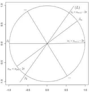
where ki = Ψ(i)−Υ(i), Ψ(i) = #{j: 0≤αj < αi+π} and Υ(i) = #{j : 0≤αj < αi},
and αi is the angle of ui = (Xi −x)/||Xi−x||. We can assume 0 = α1 ≤... ≤ αm < 2π
and αm+1 =α1+ 2π, αm+2=α2+ 2π, and so on (see Figure 2). To reduce the calculation
time of Ψ, the authors use an updating mechanism that sorts the array consisting of αi’s
and their opposite angles βi =αi+π. Then Ψ(1) = #{j: 0≤αj < π=β1} and Ψ(2) =
Ψ(1) + #{αj’s lying between β1 and β2}. Similarly, Ψ(3) = Ψ(2) + #{αj’s lying between β2 and β3}, and so on. We illustrate this procedure with two simple examples.
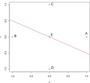
Example 1: Let the reference sample consist of four pointsA, B, C, D be (±1,0),(0,±1), and consider the point E = (0,0). We will calculate the depth of E by both the intuitive way and also via Rousseeuw and Ruts’ (1996) method. Without performing any difficult computations, we can see that E has depth 1/2 because there are only two possibilities where a line passes throughE. Either it coincides with one of the two axes, or it doesn’t, as in Figure 1. For the first case, the minimum proportion of reference points on one side of the line is 1/2, and for the second case it is 3/4. To find the depth via the method of Rousseeuw and Ruts, we first, calculateα1, α2, α3, α4,which are angles of vectors −→EA, −−→EB, −−→EC, −−→ED
with respect to the x-axis. So α1 = 0, α2 = π/2, α3 = π, α4 = 3π/2, Υ(i) = i−1 and
Ψ(1) = 2, Ψ(2) = 3, Ψ(3) = 4, Ψ(4) = 5.Hence k1 =k2 =k3 =k4 = 2, and the depth is
indeed 1/2 (see Figure 2).
To explain the three-dimensional case, we build on what we showed for two dimensions in the last example. The main idea is to reduce the problem to the two-dimensional case by projecting all the reference points onto a plane. The chosen plane is perpendicular to the line connecting x and one of the reference points. Then, we use the computational method for the two-dimensional case to find the depth ofxon this plane. The three-dimensional depth
Figure 1: Tukey depth in two-dimensional space
is the smallest two-dimensional depth amongst all projections (we have different projections when we choose different reference points to connect with x).
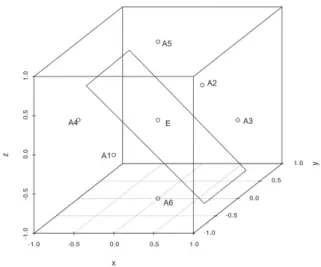
Example 2: Similar to Example 1, the reference sample consists of six pointsA1, ..., A6 on
(±1,0,0),(0,±1,0),(0,0,±1). We calculate the depth ofE = (0,0,0) by both an intuitive way and Rousseeuw and Ruts’ method. The intuitive way to calculate the depth now is by rotating a plane around the point E. This is now much harder to imagine, especially to cover all possibilities for the plane, but the result is the same as in Example 1. If the plane passing through the originE does not pass through any of the reference points, then it separates the points in half, with three on each side (see Figure 3). Otherwise, the plane contains at least one coordinate axis (the plane passes the origin and a point on an axis) and the minimum proportion of points on one side of the plane will be 5/6. So the depth of E in this case is also 1/2.
To implement the method of Rousseeuw and Ruts, we first connect E with A1, which
is the x−axis (denote by L in general). We denote γ to be the plane passing through E
and perpendicular to L (this is the yz−plane). Then, we project all reference points onto
γ.The resulting points are the same as in Example 1, along with these added points
m0 = #{points whose projections coincide with E}= 0,
m+= #{points lying aboveγ whose projections coincide with E}= 1, m−= #{points lying belowγ whose projections coincide with E}= 1,
Figure 2: Illustration of angles in calculating two-dimensional Tukey depth
plane η passing throughE is
T DGm(E) = 1 m [ min i {min (ki,m˜ −ki)}+ min { m+, m−}+m0 ] = 1 6[2 + 1 + 0] = 1 2, whereki’s are calculated as in Example 1 for two-dimensional case.
The approximation algorithm forp-dimension (p≥4) is based on a generalization of the same process of projecting our reference sample into a subspace of the higher dimensions in order to reduce the dimension. In particular, the method that Rousseeuw and Ruts (1996) proposed was to project the whole reference sample set onto a line which is chosen using the steps below. After the projection, we calculate the Tukey depth in one dimension, which is the smallest proportion of the reference sample on either side of the line separated by the point whose depth we are calculating. The approximation is a multi-step algorithm that is repeated ktimes. Let T DGm(x) =m and repeat the following five steps:
1. Draw a random sample of size pfrom the reference points. 2. Determine a direction uperpendicular to the p-subset.
3. Project all data points on the line Lthrough x with directionu. 4. Compute the univariate depthdof xon L.
5. UpdateT DGm(x) = min{T DGm(x), d}. This approximation is the smallest univariate depth ofxamongst all considered projections.
Figure 3: Tukey depth in three-dimensional space
5.3 Choosing the best method
At first glance, there is no obvious “best choice” of which data depth measure to use in mul-tivariate control charts. Zuo and Serfling (2000) considered a wide range of depth functions and compared them using their four key properties listed in the last section. Simplicial depth has appealed to researchers in part due to its intuitive geometric interpretations. It is not hard to find counterexamples showing that simplicial depth fails to satisfy the second and third criterion for some discrete distributions. For example, consider the univariate point mass function: P(X = 0) = P(X = ±1) = P(X = ±2) = 1/5. In this case, all intervals containing 1/2 will contain 1, however the interval [1,2] contains X = 1 but not X = 1/2, so the depth at X = 1 is larger than depth at X = 1/2. This violates the principal of monotonicity relative to deepest point (0 in this case).
A data depth measure is also judged on its computational feasibility, especially with regard to high-dimension problems. Rousseeuw and Ruts (1996) and Rousseeuw and Struyf (1998) provided FORTRAN codes to calculate the Tukey depth for bivariate and trivariate data, as well as an approximation procedure with much faster calculation time for higher dimensions. Their results also compute simplicial depth for bivariate data with comparable computing time to that of Tukey depth. This calculation time required for bivariate data was confirmed to be as good as possible by Aloupis et al. (2002). Other attempts to reduce the calculation complexity in higher dimensions includes Cuesta-Albertos and Nieto-Reyes (2008), where they estimated the Tukey depth by the so-called “random Tukey depth”, which requires much less computational time under certain conditions. Another result is
an output-sensitive algorithm for half-space depth by Bremmer et al. (2008), where they introduced an algorithm calculating Tukey depth in three or more dimensions. The running time of these algorithms depends on the actual depth needed to be calculated.
In addition to these considerations, an effective data depth function should have a high breakdown point. The breakdown point represents the upper limit of bad data (in terms of a fraction) that the depth function can handle before it will give an arbitrarily bad result. In this regard, Tukey depth is considered better than most other depth functions. Its cor-responding location estimator has breakdown point 1/3 for typical data sets, while location estimator for the spatial depth has breakdown point 1/2 (Liu et al., 2013). In general, the simplicial depth performs adequately with continuous distributions, even though the estimator based on simplicial depth has breakdown point 0.
Overall, we can observe that both Tukey depth and simplicial depth have been studied thoroughly, and the Tukey depth function has obvious advantages in terms of the key properties, e.g., computational feasibility and breakdown point.
5.4 Control Charts based on Data Depth
The first distribution-free multivariate control charts using data depth introduced by Liu (1995) were based on the simplicial depth. Until now, several depth-based control charts have been suggested, and among them, well-known control charts based on the data depth are
• r-chart: Shewhart-type chart for individual measurements • Q-chart: Shewhart-type chart based on means of subsamples • S-chart: CUSUM-type chart.
Stoumbos et al. (2001) noted that theQ-chart denotation risks being confused with short production run control charts by Quesenberry (1991). Liu (1995) illustrated these charting methods with simplicial depth and Mahalanobis depth, but they can be easily extended to Tukey depth. Suppose that the data consist of a set of reference samples {y1, . . . ,ym}
governed by a prescribed continuousp-dimensional distributionG withGm being the
cor-responding empirical distribution. The new observations{x1,x2, . . .}are assumed to follow
a distributionF. Based on the observations xi’s, we determine whether the process is out
of control by comparingF with the distributionG.
Liu’s r-chart is based on depth function DG(·) in the statistic: rG(x) = P{DG(y) ≤ DG(x)|y ∼G},where y∼Gindicates that yfollows the distribution G. If G is unknown
and the reference sample {y1, . . . ,ym} are only available, then the r-chart is constructed
based on
rGm(x) =
#{yj|DGm(yj)≤DGm(x)}
m . j= 1, . . . , m. (8)
rGm(·) reflects how close thep-dimensional vectorxis to the center of the data cloud created by the reference sample. Ther-chart plots the valuesrGm(xi) against timeiwith CL = 0.5 and a lower control limit (LCL), say α. The process is considered out of control if the
rGm(xi) statistic is smaller than α.
To construct the Q-chart (analogous to the Shewhart ¯X-chart), Liu (1995) presented a simple extension to the r-chart. Let Fn(·) denote the empirical distribution of the sample
{x1, . . . ,xn}and define QG(F) =P{DG(y)≤DG(x)|y∼G,x∼F}.The Q-chart is based
on the Qstatistic QG(Fn) = 1 n n ∑ i=1 rG(xi) or QGm(Fn) = 1 n n ∑ i=1 rGm(xi) (9)
ifG is unknown. The Q-chart plots {QG(Fn1), QG(Fn2), . . .} or {QGm(F
1
n), QGm(F
2 n), . . .}
if only reference sample {y1, . . . ,ym} are available, where Fnj is the empirical distribution
of the jth subset of size n from the new observations. The Q statistic averages out the r
statistics in subsets to prevent a single fluctuation from giving a false-positive alarm. The
Q chart has the CL = 0.5 and a lower control limit of LCLQ = n−1(n!α)1/n for small
subsamples ofn≤4 under the assumption ofα= 0.01 since the general condition for using that LCL is α≤1/n!, and for n≥5,
LCLQG= 0.5−zα(12n) −1/2 and LCL QGm = 0.5−zα √ 1 12 ( 1 m + 1 n ) .
The S-chart is motivated from the CUSUM chart with the intention of detecting small process shifts by accumulating the deviations from the expected value. In the multivariate setting, Liu and Singh (1993) used the statistic
Sn(G) = n ∑ i=1 (rG(xi)−1/2) or Sn(Gm) = n ∑ i=1 (rGm(xi)−1/2)
for plotting{S1(G), S2(G), . . .}or{S1(Gm), S2(Gm), . . .}ifGis unknown and only random
sample{y1, . . . ,ym}are available. The chart’s lower control limit is LCLSG =−zα(n/12)−
1/2 and LCLSGm =−zα √ n2 12 (1 m + 1 n )
.A standardized version, calledS∗n(G) andSn∗(Gm) chart,
are based on S∗n(G) = √Sn(G) n/12 and S ∗ n(Gm) = Sn(Gm) √ n2(1/m+ 1/n)/12.
so the lower control limits do not depend on m or n. This S∗ chart has CL = 0 and LCL = −zα. As a result, the S∗-chart has a horizontal control limit and a smaller, more
practical chart size.
Besides, Liu et al. (2004) proposed a data depth based moving-average (DDMA) control chart for monitoring multivariate data. The DDMA chart is a nonparametric multivariate control chart derived from the notion of data depth which is devised to detect simultaneously process changes in location and scale. For the new observations{x1,x2, . . . ,xn}, the DDMA
chart monitors the moving averages with length q, i.e., ˜xq = (x1 +· · ·+xq)/q, ˜xq+1 =
(x2 +· · ·+xq+1)/q, . . ., ˜xn = (xn−q+1 +· · ·+xn)/q. Let ˜X = {˜xq, . . . ,x˜n}. Then the
corresponding reference samples for monitoring ˜xi ∈ X˜ is ˜Y = {y˜q, . . . ,y˜m} such that
˜
yq = (y1+· · ·+yq)/q, ˜yq+1 = (y2+· · ·+yq+1)/q, . . ., ˜ym= (ym−q+1+· · ·+ym)/q. For
each ˜xi∈X˜, its relative rank is calculated with respect to {y˜q, . . . ,y˜m}, i.e.,
rG˜m−q+1(˜xi) = # { ˜ yj|DG˜m−q+1(˜yj)≤DG˜m−q+1( ˜xi) } m−q+ 1 , j=q, . . . , m. (10)
where ˜Gm−q+1 is the empirical distribution of ˜Y, and DG˜m−q+1(·) is the empirical depth
computed with respect to ˜Gm−q+1. The DDMA chart plotsrG˜m−q+1(˜xi) against the indices i=q, . . . , n with CL = 0.5 and LCL =α.
5.5 Curse of Dimensionality
A primary step of statistical process is to create a reference sample large enough to gain sufficient evidence that the process is actually in control. The reference sample serves as the benchmark for judging future process outputs, so insufficient reference sample can potentially disqualify the results of any control chart that follows. This is a critical problem with multivariate data, where the increased dimension of the data creates an unavoidable sparseness within the reference sample. Without the features of a parametric model that conveniently relate distant observations, it is hard to deduce how new observations relate to the bench-marked data in the reference sample unless they happen to be close neighbors in multivariate space.
Liu (1995) discussed requirements for the reference sample size, which can be as small as 50 for bivariate data but much larger for higher-dimensional cases. This heuristic claim has been discussed in detail by Stoumbos et al. (2001). In that paper, the authors did a thorough study on the effect of the reference sample size (m) on Q-charts using different subgroup sizes (n= 1, ...5). Stoumbos et al. (2001) pointed out a fatal problem with these nonparametric charts: the data can be so sparse in p ≥ 3 dimensions that a lot of the reference data are likely to be “on the outside” in that they will seem to be extreme in at
least one dimension. They focused on average run length (ARL) of an in-control process and showed that it might be impossible to find a positive threshold (e.g., r(X) ≤ α for the r-chart) that can create a valid chart with a reasonable ARL. A 3σ Shewhart chart garners a false alarm rate (FAR) of P(|N(0,1)| > 3.0) = 2(1−Φ(3)) = 0.0027 and a corresponding ARL of 1/0.0027 = 370.4. If the reference sample is not large enough, a typical nonparametric chart will report an ARL much smaller than 370 by rejecting only the most outlying data points in the sample.
To factor this in the problem, Stoumbos et al. (2001) computed the ARL at the expected minimum positive false alarm rate based on finding the expected number of points that will be on the outside border of the reference sample. The expected number of extreme points increases with the number of variablespbut also changes with the reference distributionG
and distribution F. They considered p of 2 and 3, generating data from the multivariate normal distribution and uniform distributions on unit circle and unit sphere, respectively. The findings reveal something we might already suspect: individual control charts based on data depth are not a practical option unless the reference sample is enormous (perhaps larger than 10,000). By subgrouping data in group sizes ofn≥3, we can achieve effectively high ARL values for trivariate data (p = 3) if the reference samples are larger than 500. Stoumbos et al. (2001) recommend 600≤m ≤1000, depending on the distribution of the data.
Although these findings are based on applications using simplicial depth, the findings are the same with Tukey depth. Reference sample requirements are based on the number of extreme points in their expanded reference sample (see equation (2) of Stoumbos et al., 2001), which is the same for both depth functions.
6
Numerical Example
We rely on Monte Carlo simulation to show how well the data depth-based control charts fare versus traditional charts when analyzing multivariate process data. We compare the performances of four data depth-based control charts, that is,r-chart,Q-chart,S-chart, and DDMA chart, to those of a T2 chart in terms of the accuracy of process change detection. For our example we consider a p = 5 variable process that is in control with observations generated from a Weibull distribution having a distribution functionF(x) = 1−exp(−(λx)κ) with parameter valuesκ= 1.5 andλ= 1.0, which has mean and standard deviation of 0.9027 and 0.6130, respectively. The process will be out-of-control after 40 observation periods, at which time the five variables are generated from an Exponential(λ= 1) distribution, with shifted mean and standard deviation of (1.000, 1.000). That is, the process suffers a small
location shift along with an increase in variability.
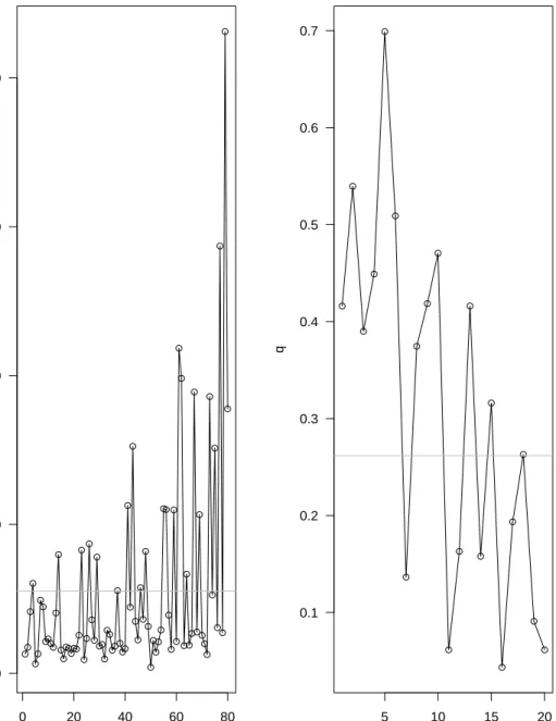
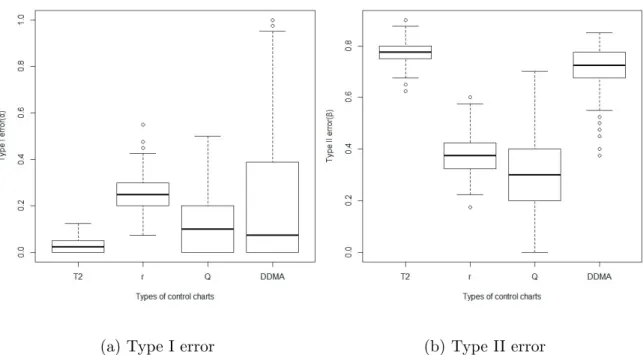
The simulations are based on 500 reference samples from the in-control distribution. To measure the effectiveness of the competing charts, we repeat each simulation 500 times and keep track of the type I errors (in the first phase) as well as the type II errors (in the out-of-control phase). Both tests are calibrated to have nominal type I error of α = 0.05. One set of charts from the simulations appears in Figure 4.
The parametric (T2) chart in Figure 4 plots 80 points, with the first 40 representing
T2 statistics from the in-control process. The chart is considered to be out of control if the T2 statistic exceeds 11.0705. The nonparametric Q-chart (based on Tukey depth) has only 20 observational periods because subgroups of n=4 are required to make the chart effective. The chart is ruled to be out of control if the test statistic (Q) is less than 0.2617. The results of the entire set of 500 simulations are summarized by the box-plots in Figure 5. The S-chart is a CUSUM-type chart accumulating the deviations from the expected value and the type II error will be relatively small due to the nature of simulation. Thus, we exclude the results from the S-chart for the purpose of comparison. The data depth based charts are more effective in this example, although the type I error rates from the nonparametric charts are higher than that from the T2 chart. After the charts are out of control, the type II errors from the nonparametric charts are remarkably small, for instance, only 30% (seven of ten observations are ruled out of control) forQ-chart compared to 77% for T2 chart. The Q-chart has the median of type I error being αQ = 0.10, and 50% of
the simulations producing type I error rates between 0 and 0.20. The T2 is only slightly more biased, with median type I error rate of αT2 = 0.0285, and 50% of the simulations
producing type I error rates between 0 and 0.05.
After the process becomes out of control, the nonparametric charts prove to be much more effective in detecting the changes. The Q-chart detects the shift, on average, 70.82% of the time (50% of the simulations producing type II error rates between 0.20 and 0.40). In contrast, the parametric chart detects the shift only 22.54% of the time, on average (50% of the simulations producing type II error rates between 0.75 and 0.80). However, the type II error from the DDMA chart is comparably large: the DDMA chart detects the shift only 29.01% of the time, on average (50% of the simulations producing type II error rates between 0.675 and 0.775). The simulation results are not unlike other comparisons between nonparametric and parametric charts (Chakraborti et al., 2001). The parametric procedures tend to underestimate the type I error, while the power to detect an out-of-control process is greatly decreased, compared to the nonparametric chart. In this case, the type II error doubles that of the nonparametric chart when the process means and variances
are shifted.
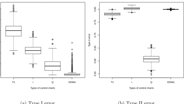
To show that the performance of the nonparametric charts improves as the reference sample size increases, we perform the simulation again with 2500 reference sample points and 4000 observations where the first 2000 points are in-control and the last 2000 observa-tions are out-of-control, using the same distribuobserva-tions as before. The summary of results is presented in Figure 6. In this case, the bias of the parametric chart becomes significantly worse without showing improvement with type II error: theQ-chart detects the shift 39.28% of the time, while the parametric chart detected the shift 21.87% of the time, on average.
7
Discussion
The purpose of this article is to summarize recent research results for constructing mul-tivariate, nonparametric control charts. Rather than relying on the linear reduction of principal components analysis, we focus on dimension reduction via the computational in-tensive methods of data depth. Specifically, we used the method by Rousseeuw and Ruts (1996) for computing Tukey depth, which has several important advantages over the other depth functions.
Multivariate nonparametric control chart research still has a long way to go before they will be considered effective enough to gain wide use. We feature Shewhart-type charts for subgroup sizes of n ≥3, noting that individuals charts are highly impractical because we cannot count on obtaining reference samples large enough (typically in the thousands) to ensure that the type I error rate of the chart will be controlled.
In some cases, nonparametric charts are strictly necessary, but if standard parametric charts are viable in multivariate settings, the more complicated nonparametric charts should be considered as a last resort. Unlike the simpler univariate settings, the loss of efficiency that is associated with distribution-free statistical inference might be substantial with mul-tivariate data, in part due to the curse of dimensionality. For detecting slow or moderate shifts in the process target mean, it has been generally known that the multivariate version of the EWMA is robust to non-normal data, so that nonparametric alternatives may be less necessary.
References
[1] Albers, W. and Kallenberg, W.C.M. (2004) Empirical non-parametric control charts: estimation effects and corrections.Journal of Appled Statistics,31, 345–360.
0 20 40 60 80 0 20 40 60 80 Index TT 5 10 15 20 0.1 0.2 0.3 0.4 0.5 0.6 0.7 Index q
Figure 4: Example of (a) T2 control chart and (b) nonparametric Q-chart for example with 80 periods of observedp=5 variate data. The process becomes out of control after 40 periods.
(a) Type I error (b) Type II error
Figure 5: Box plots summarizing Type I and Type II errors for the parametric and non-parametric control charts with 500 reference points and 80 observations. The first box plots represent type I error for the T2 chart, r-chart, Q-chart, and DDMA chart. The next box plots represent type II errors for the same.
T2 r Q DDMA 0.000 0.005 0.010 0.015 0.020 0.025 0.030
Types of control charts
T
ype I error
(a) Type I error
T2 r Q DDMA 0.55 0.60 0.65 0.70 0.75 0.80
Types of control charts
T
ype II error
(b) Type II error
Figure 6: Box plots summarizing Type I and Type II errors for the parametric and non-parametric control charts with 2500 reference points and 4000 observations. The first box plots represent type I error for theT2 chart, r-chart,Q-chart, and DDMA chart. The next box plots represent type II errors for the same.
[2] Aloupis, G., Cortes, C., Gomez, F., Soss, M. and Toussaint, G. (2002) Lower bounds for computing statistical depth.Computational Statistics & Data Analysis,40, 223–229. [3] Alt, F.B. (1984) Multivariate quality control, inThe Encyclopedia of Statistical Science,
Kotz, S., Johnson, N.L. and Read, C.R. (eds), John Wiley, New York, 110–122. [4] Alt, F.B. and Smith, N. (1988) Multivariate process control, inHandbook of Statistics,
Vol. 7, Krishnaiah, P.R. and Rao, C.R. (eds), Elsevier, Amsterdam, 333–351.
[5] Altukife, F.S. (2003a) A new nonparametric control charts based on the observations exceeding the grand median.Pakistan Journal of Statistics,19, 343–351.
[6] Altukife, F.S. (2003b) Nonparametric control charts based on sum of ranks. Pakistan
Journal of Statistics,19, 291–300.
[7] Amin, R.W., Reynolds, M.R. Jr. and Bakir, S.T. (1995). Nonparametric quality control charts based on the sign statistic.Communications in Statistics - Theory and Methods,
23, 1597–1623.
[8] Amin, R.W. and Searcy, A.J. (1991) A nonparametric exponentially weighted moving average control scheme.Communications in Statistics - Simulation and Computation,
20, 1049–1072.
[9] Arts, G.R.J. Coolen, F.P.A. and Van Der Laan, P. (2004) Nonparametric predictive inference in statistical process control. Quality Technology and Quantitative Manage-ment,1, 201–216.
[10] Bakir, S.T. and Reynolds, Jr., M.R. (1979) A nonparametric procedure for process control based on within-group ranking.Technometrics,21, 175–183.
[11] Bakir, S.T. (2004) A distribution-free Shewhart quality control chart based on signed-ranks.Quality Engineering,16, 613–623.
[12] Bakir, S.T. (2006) Distribution-free quality control charts based on signed-rank-like statistics.Communications in Statistics - Theory and Methods,35, 743–757.
[13] Balakrishnan, N., Triantafyllou, I.S. and Koutras, M.V. (2009) Nonparametric control charts based on runs and Wilcoxon-type rank-sum statistics. Journal of Statistical
Planning and Inference,139, 3177–3192.
[14] Barnett, V. (1976) Ordering of multivariate data.Journal of the Royal Statistical
[15] Bersimis, S., Psarakis, S. and Panaretos J. (2007) Multivariate statistical process con-trol charts: an overview.Quality & Reliability Engineering International,27, 517–543. [16] Boone, J.M. and Chakraborti, S. (2012) Two simple Shewhart-type multivariate non-parametric control charts. Applied Stochastic Models in Business and Industry, 28, 130–140.
[17] Bodden, K.M. and Rigdon, S.E. (1999) A program for approximating the in-control ARL for the MEWMA chart.Journal of Quality Technology,31, 120–123.
[18] Borror, C.M., Montgomery, D.C. and Runger, R.C. (1999) Robustness of the EWMA control chart to non-normality.Journal of Quality Technology,31, 309–316.
[19] Bremmer, D., Chen, D., Iacono, J., Langerman, S. and Morin, P. (2008) Output-sensitive algorithms for Tukey depth and related problems.Statistics and Computing,
18, 259–266.
[20] Bush, H.M., Chongfuangprinya, P., Chen, V.C.P., Shkchotrat, T. and Kim, S.B. (2010) Nonparametric multivariate control charts based on a linkage ranking algorithm.
Qual-ity and ReliabilQual-ity Engineering International,26, 663–675.
[21] Camci F., Chinnam R.B. and Ellis R.D. (2008) Robust kernel distance multivariate control chart using support vector principles.International Journal of Production
Re-search,46, 5075–5095.
[22] Chakraborti, S., Van Der Laan, P. and Bakir, S.T. (2001) Nonparametric control charts: an overview and some results.Journal of Quality Technology,33, 304–315.
[23] Chakraborti, S. and Van de Wiel, M.A. (2003) A nonparametric control chart based on the Mann-Whitney statistic. SPORreportNo.2003-24. Department of Mathematics and Computer Science, Eindhoven University of Technology, Eindhoven, The Netherlands. (The paper is available in www.win.tue.nl/bs/spor/2003-24.pdf).
[24] Chakraborti, S., Van Der Laan, P. and Van de Wiel, M.A. (2004) A class of distribution-free control charts.Journal of the Royal Statistical Society, Series C: Applied Statistics,
53, 443–462.
[25] Chakraborti, S. and Eryilmaz, S. (2007) A nonparametric Shewhart- type signed-rank control chart based on runs.Communications in Statistics - Simulation and Computa-tion,36, 335–356.