Flexible Option Valuation Methods

(1)

Flexible Option Valuation Methods

Yun YIN School of Economics University of East Anglia

A thesis submitted for the degree of Master of Philosophy

This copy of the thesis has been supplied on condition that anyone who consults it is understood to recognise that its copyright rests with the author and that use of any information derived there from must be in accordance with current UK Copyright Law. In addition, any quotation or extract must include full attribution.

(2)

Abstract

This thesis is concerned with methods of option valuation that fall completely outside of the Black-Scholes-Merton (BSM) framework. Data on S&P500 Index options are used to demonstrate the proposed methods. Some of our favoured methods are based on semi-parametric regression; others on simulation. The thesis consists of a number of chapters. In Chapter 2, we outline existing option valuation methods, with particular attention paid to the binomial-tree model and the Black-Scholes formula. We demonstrate that under some circumstances these two methods are equivalent. We also demonstrate using the binomial tree method that a “TGARCH effect” (which plays an important role in later chapters) can explain the well-known “smirk” pattern that is often observed in market option price data.

In Chapter 3, we use regression analysis to investigate the ways in which features of an option actually determine the market price. We start with polynomial regressions, and progress to additive models, with components obtained using the B-spline technique. The focus in these regression models is the role of volatility. Historical measures of volatility are used as explanatory variables in the regression, with one objective being to discover how far back into the past option traders are going when computing volatility. It is proposed that this approach gives rise to an alternative measure of implied volatility that is completely free of the Black-Scholes framework. We use the Practitioner Black Scholes (PBS) model as a Benchmark for comparison. The best of our regression models is found to perform better than the Black-Scholes formula in out-of-sample prediction of market prices.

In Chapter 4, we focus on the underlying (S&P500) Index, and consider a number of varying volatility models (ARCH, GARCH and TGARCH) of daily returns. We found that the TGARCH model is the best model to represent the volatility process. Then we simulated data from the models considered using the coefficients from the estimated models. After that, we found that the simulated ARCH family volatility models worked correctly, since the “true” parameter values are included in the confidence intervals.

Chapter 5 continues with the simulations of daily return data, in building a Monte Carlo program for the valuation of European options that allows for varying volatility. Of particular interest is whether superior models of the underlying stock price (i.e. ARCH, GARCH and TGARCH) result in option valuations that are superior to the Black-Scholes valuation. Superiority in this context is defined primarily in terms of ability to predict market prices. We find that all models perform better than the benchmark (PBS) model. Which model performs best depends on the type of market and time to

(3)

expiry: ARCH is the best model for predicting the short and medium term put options for both bear and calm market and GARCH is the best one for predicting the long term put options in the bear market. In the crash market, TGARCH Monte Carlo simulation is the best model for predicting the long term European call and put options.

(4)

Acknowledgement

Firstly, I would like to express my sincere gratitude to my supervisor Professor Peter Moffatt for the continuous support of my PhD study and related research, for his patience, motivation, and immense knowledge. His guidance helped me throughout the time of the research and the writing of this thesis. I could not have imagined having a better supervisor and mentor for my PhD study.

Besides my supervisor, I would like to thank the rest of my thesis committee, Dr. James Watson and Dr. Bahar Ghezelayagh, for their insightful comments and encouragement, and also for the hard questions which prompted me to widen my research from various perspectives. Special thanks also go to my family. Words cannot express how grateful I am to my mother and father for all of the sacrifices that you’ve made on my behalf. Your prayer for me was what sustained me thus far. I would also like to thank all of my friends who supported me in writing, and encouraged me to strive towards my goal.

I am also very grateful to the examiners, Dr Panayotis Andreou and Dr Marta Wisniewska, for supplying excellent feedback on earlier versions of the thesis.

(5)

List of Figures

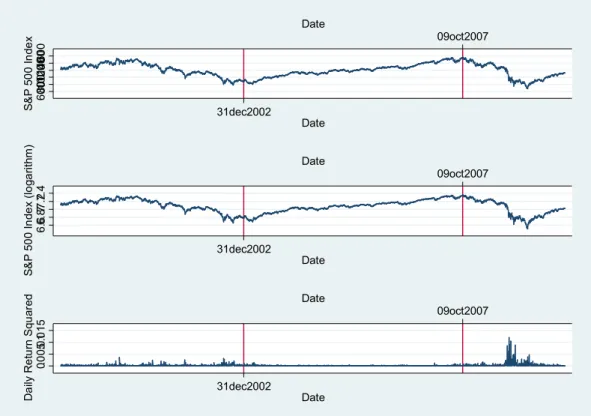
Figure 1.1 Time path of S&P 500 (daily data), daily return of S&P 500 and

the squared daily return (volatility) of S&P 500; 1 Jan 2000 – 31 Oct 2009..8

Figure 2.1 Payoff diagram for a Call Option with strike K...16

Figure 2.2 Payoff diagram for a put option with strikeK...16

Figure 2.3A two-step Binomial Tree...18

Figure 2.4 A one-step Binomial Tree...19

Figure 2.5 Binomial Tree on-line Calculator...22

Figure 2.6 Binomial Tree on-line Calculator Result with 2 steps...23

Figure 2.7 Binomial Tree on-line Calculator Result with 10 steps...23

Figure 2.8 A two-step Binomial Tree example...24

Figure 2.9 (a) A two-step binomial tree with simple random walk assumption...26

Figure 2.10 (b) A two-step binomial tree with TGARCH assumption...27

Figure 2.11 Time Path of S&P 500 Index...36

Figure 2.12 Time-Series of daily volatility...36

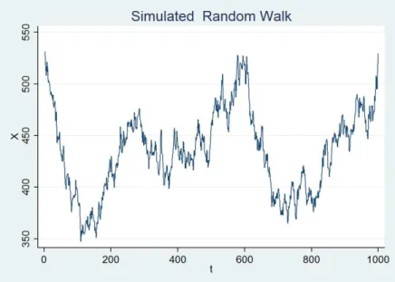
Figure 2.13 Simulated Random Walk...37

Figure 2.14 Simulated “Black-Scholes” series...38

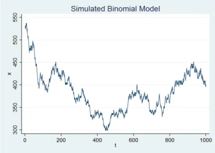
Figure 2.15 Simulated Binomial Model...38

Figure 3.2 Basis Functions with four knots...50

Figure 3.3 Basis functions for moneyness...51

Figure 4.1 The return series and the closing prices against time from 1 January 2000, through 31 October 2009...71

Figure 4.2 Autocorrelations of daily S&P500 returns for up to two years...73

Figure 4.3 Histogram of daily S&P500 returns and the normal distribution74 Figure 4.4 Autocorrelation of squared daily S&P500 returns for up to 504 days...76

Figure 4.5 S&P500 Index (logarithm) and returns squared...76

(8)

Figure 4.7 Conditional variances (from top to bottom: ARCH, GARCH, TGARCH), one-step ahead...85 Figure 4.8 Scatter plots of conditional volatilities against each other, obtained after fitting each models for S&P500 returns...86 Figure 4.9 S&P500 prices (logarithm)...87 Figure 4.10 Autocorrelation of squared returns for each market separately ...88 Figure 6.1 Four simulations of TGARCH models...104 Figure 6.2 Early exercise boundary obtained from 100 simulated paths of the TGARCH model...104 Figure 6.3 Early exercise boundaries from the four different models...105

(9)

List of Tables

Table 1.1 Sample descriptive statistics by time period and time to expiry...9 Table 2.1 Information for the Option Example...24 Table 2.2 Binomial Tree on-line Calculator Result Results with different numbers of tree-steps...25 Table 2.3 Comparison results of simple random walk with TGARCH...28 Table 2.4 Greeks of Black-Scholes Call Formula...33 Table 2.5 Value of European Options of Black-Scholes formula and Binomial Model...39 Table 3.2 Polynomial Regression Results for complete set of put options. Dependent variable: put option price...48 Table 3.3 B-spline Regression Resultswith different measures of volatility. Dependent variable: put option price...53 Table 3.4 Volatility coefficients from B-spline Regression models estimated separately by time period and time to expiry...54 Table 3.5 B-spline Regression Results with 60-days range of volatility and 60-days range of skewness. ...56 Table 3.6 Box-Cox regression results for all put options and all call options ...60 Table 3.7 In-sample and out-of-sample pricing performance of (Box-Cox) Linear Regression, (Box-Cox) Quadratic Regression, (Box-Cox) Cubic Regression, (Box-Cox) B-spline Regression, PBS, and PBS with Smearing (PBS_S)...61 Table 3.8 In-sample and out-of-sample pricing performance of five IV equations for both call and put options...64 Table 3.9 In-sample and out-of-sample pricing performance of PBS using different DVF models of both call and put options. ...65 Table 3.10 Average Profits of each model using the different data set with hedging strategy...错误！未定义书签。 Table 3.11 Average profits of each model using the different data set without hedging...错误！未定义书签。 Table 4.1 Summary Statistics of daily return, S&P500...75

(10)

Table 4.2 Estimated models for the daily returns of SP500 index under generalised errors...84 Table 4.3 Summary statistics of the data across the three ranges...87 Table 4.4 Parameter Estimates from ARCH, GARCH and TGARCH models..90 Table 5.1 Numbers of options used in the Monte Carlo simulation...94 Table 5.2 Pricing Performance for the whole data set...99 Table 5.3 Pricing Performance of all models with different markets: Bear Market (2002), Calm Market (2005) and Crash Market (2008)...99 Table 5.4 Pricing Performance of all models of three markets with three maturity range: short term options, medium term options and long term options...99

(11)

Chapter 1 Introduction

Options are financial instruments that can provide investors with the flexibility needed in a wide variety of investment situations. Although the history of options extends several centuries, a formal market for options was not established until the Chicago Board Options Exchange (CBOE) opened its doors in 1973.In the same year, two economists, Fischer Black and Myron Scholes, published an article proposing a model for calculating the theoretical estimate of an options price over time. Also in the same year, their colleague Robert Merton published an additional study providing a mathematical extensions of the Black-Scholes model.

With an exchange created and a solid model for pricing, the market flourished. New options contracts were issued subject to standardized terms, such as uniform expiry dates and established strike prices. The Options Clearing Corporation (OCC) became the central clearing house, which guaranteed trades, and was responsible for regulatory oversight on par with U.S. stock markets.

In 1973, options trading at the CBOE was restricted to call options in only 16 stocks.Over time, the listed options market expanded to additional exchanges and products, including put optionsand index options.

The popularity of options has steadily increased. The US is the largest option trading market, with total trading volume on U.S. options exchanges being 4.14 billion contracts in 2015 (16.4 million contracts per day).1 However, the popularity of options has spread over the world. In the UK, the London International Financial Futures Exchange (LIFFE) introduced equity options to its product range in 1993. China eventually launched stock options on 9th_{February 2015, aiming to develop broader markets and} give investors a tool to manage risk. The options were written on an exchange-traded fund, the China ETF, which tracks 50 of China’s largest listed firms, including banking giant ICBC and carmaker SAIC Motor.

Options are useful in hedging, since when held in conjunction with other assets, loss from holding the portfolio can be avoided with certainty. They are also useful for speculators: it is possible to make large profits by searching for favourably priced options, and then either holding them to expiry or selling them at a profit at some time before expiry.

Whether the trader is a hedger or a speculator, they need reliable methods for valuing options.If a hedger is purchasing an option in order to create a hedge, they need to know that the offer price is close to the true value of the option, otherwise the portfolio might result in a net loss. If the trader

(12)

is a speculator, an obvious strategy is to buy options for which the true value is higher than the offer price, and sell options for which the true value is less than the bid price.

Option valuation methods are usually related in some way to the Black-Scholes-Merton (BSM) framework (Black and Scholes, 1973; Merton, 1973). This framework is built on the assumption that the underlying asset price follows a geometric Brownian motion process with constant return volatility (or a random walk). Another key assumption is risk-neutral arbitrage. The great advantage of the BSM framework is that the value of certain options (e.g. European options) can be expressed in closed form, and the formula can be easily applied. Because of this, the BSM approach has become the industry standard in recent decades.

In 1997, the importance of this contribution was recognized when Robert Merton and Myron Scholes were awarded the Nobel Prize for Economics. Robert Merton, among many others, extended the Black-Scholes model in several important ways.As these studies have shown, option pricing theory is relevant to almost every area of finance.

While fully acknowledging the hugely significant contribution of Black, Scholes and Merton, the overall message of this thesis is that there is perhaps too great a reliance on the BSM framework. The main problem is that it is based on the assumption of constant return volatility of the underlying asset.There is a vast literature in Financial Econometrics establishing that this assumption is usually false. In addition, it is often suggested that the well-known “smiles” and “smirks” seen in option price data are a consequence of the violation of this assumption. Some authors have attempted to extend the Black-Scholes framework to incorporate varying volatility.In this thesis, we instead focus on option valuation methods that are completely outside of the Black-Scholes framework. One method is based on regression; the other is based on simulation.

Another message of the thesis relates to the question: what are option valuations actually useful for? For example, the predicted valuations from a regression model may be compared to actual option prices and hence a measure of the predictive performance of the model can be obtained. Predictive performance is clearly important in, for example, setting prices for options in thinly traded markets. Another use of option valuations is in the development of profitable trading rules. The decision to purchase an option is made on the basis of a comparison between the valuation and the market price. Purchased options may then be combined with appropriate units of the underlying to form a hedged portfolio. The average performance of the hedged portfolios can then be used as a measure of the performance of the model.

(13)

1.1 A broad framework

Here we will introduce a broad framework to which most of the analysis of the thesis can be related. We will not provide complete definitions here -this will be done in Chapter 2.

An option is a security written on an underlying asset or index (often just called the “underlying”). Two basic types of option are European and American options. The fundamental difference is that European options can only be exercised at expiry, while American options may be exercised at any date on or before expiry (i.e. “early exercise” is permitted). In this thesis we will mainly be concerned with European options because they are much easier to analyse.

Consider a European call option which has price (or value) c.It is well known that c depends on a small list of variables, namely the current (time t) price of the underlying (St), the strike price (K), the time to expiry (), the

risk-free rate (rf) and the volatility of the underlying ().2 So we can write:



 



 t, , , ,f

c f S K r (1.1)

The first four arguments of f in (1.1), St, K,  andrf, are all known at timet

(the time when the option is traded.The fifth argument, , is however unknown. This means that in order to apply the formula (1.1) it is necessary to estimate the volatility of the underlying index and use this estimate (ˆ say) in place of  in (1.1). How this estimate of volatility should be obtained is one of the key issues of this thesis.

Other key ideas of the thesis can be introduced within the framework of (1.1). First of all, the binomial-tree formula and the Black-Scholes formula, which will both be derived in detail in Chapter 2, are both special cases of (1.1). Let us label the Black-Scholes formula as:



 



 _BS , , , ,_f

c f S K r (1.2)

An important concept is implied volatility, and this can be defined using (1.2).If the market price of the option isc, then the implied volatility is defined implicitly as:



 





 _BS , , , ,_f 

c f S K r (1.3)

2_{Option prices generally also depend on the dividend rate, but since we will mainly be} concerned with options written on stock market indexes, there are no dividends to consider, and the dividend rate can be assumed to be zero.

(14)

That is, the implied volatility is the volatility that is required in the Black-Scholes formula that makes the value of the option exactly equal to the market price of the option. Or, it is the volatility of the underlying asset that is implied by the market price of the option. The implied volatility is not the same as the true volatility, for two reasons: the market price of the option might not correctly represent the true value of the option; orthe Black-Scholes formula may be an invalid procedure for finding the true value of the option. Before 1987, implied volatility was a U-shaped function (known as a “volatility smile”) of the strike price, with minimum around the current price. This implies that both in-the-money and out-of-the money options were over-priced relative to at-the-money options. Since 1987, implied volatility has more commonly been a monotonically decreasing function of strike price (hence “volatility smirk”). This implies (e.g.) that in-the-money Calls are over-priced, but out-of-in-the-money calls are under-priced.

Another important topic of the thesis is regression analysis of option prices, which will be covered in Chapter 3. Here, we are performing least squares regressions with market prices of options as the dependent variable, and the five arguments off in (1.1) (and non-linear functions of them) as explanatory variables. An estimate ˆ is used in place of. We can write the fitted regression equation as:



 





ˆ LS , , , , ˆf

c f S K r (1.4)

Regression models of the form (1.4) are useful for a number of reasons. Most importantly, by experimenting with different estimatorsˆ for the volatility,, it is possible to find the estimator that optimises the fit of the regression.This optimal estimator could then be interpreted as the estimator of volatility that option traders are using when setting prices. Hence this provides an alternative means to compute the implied volatility of the option. However, unlike  in (1.3), this estimate of implied volatility is not based on the assumption that the Black-Scholes model is true. In this sense the implied volatility obtained using (1.4) is “model-free”.

All of the models considered above assume that the volatility of the underlying, , is fixed over time. Ways of relaxing this assumption are an important part of this thesis. A very important model which relaxes this assumption is the Practitioner Black-Scholes (PBS) model:

‴ ‴ㄷ ㄷh h h h h

Where h is a (usually non-linear) function of the strike price (K) and the time to expiry (τ). The PBS model is normally estimated in two stages.

(15)

Firstly, a least squares regression is performed with implied volatility as the dependent variable in order to estimate the function h . Secondly, the predicted values from this regression are plugged into the Black-Scholes formula in order to obtain predicted option prices. The PBS has become a very popular model and will be used as a benchmark model for comparison with models of interest in this thesis.

We are also interested in models in which volatility simply varies over time (such as ARCH and GARCH). Let



 

t represent a model that describes the process followed by volatility over time, and let



ˆ

 

t be the estimated volatility model (estimated using historical data on the underlying price). Then:

 



 



 _{v v} , , , , ˆ_f

c f S K r t _(1.5)

is a model of the option price that allows for varying volatility (vv).

The concept of implied volatility can be extended to varying volatility models.Let the market price of the option be c. If:

 



 





 _{v v} , , , ,_f 

c f S K r t (1.6)

then





 

t

is the implied volatility process of the option.Methods for finding





 

t

have been considered by Engle and Mustafa (1992).

1.2 Outline of thesis

Chapter 2 surveys existing option valuation methods. The most basic of these are the Binomial-tree method and the Black-Scholes method, and these two methods are derived in detail and demonstrated. It is demonstrated that under some circumstances these two methods are equivalent. It is also demonstrated that including a “TGARCH effect” in the binomial tree is a way of explaining the well-known “smirk” phenomenon seen in option price data.

Chapter 3 considers regression analysis of the market prices of options.The central question is: what features of an option actually determine the market price? Since the function that is being estimated, (1.1) above, is a highly non-linear function of certain arguments, flexible regressions are required. We will start with polynomial regressions, and progress to additive models, using B-splines for the components.Using these sorts of models, we will see that it is possible to obtain a very good fit of the data with relatively few parameters.

(16)

The regression approach is very useful for finding out which measure of volatility is being used by traders, that is, how far they appear to go back into the past when computing historical volatility. This can be answered by considering which volatility measure gives rise to the best fit in the regression.

Having estimated the regression models and identified which measure of volatility is most useful, we need to assess the performance of the model. For this purpose we will consider both in-sample and out-of-sample predictive performance. One particularly important question is whether any of the regression models can predict option prices better than the benchmark Practitioner Black-Scholes (PBS) model, used by many researchers including Christoffersen and Jacobs (2004) and Andreou (2014). Chapter 4 progresses to varying volatility models. The models considered are in theAutoregressive Conditional Heteroscedasticity (ARCH) family. In addition to ARCH itself, we consider Generalised ARCH (GARCH) and Threshold GARCH (TGARCH). We will first estimate all of these models using daily data on Index returns. We will then simulate data from the estimated models, and use the simulation routines in a Monte Carlo study of the three estimators. One reason for doing this is to verify that the simulations are being performed correctly. Another reason is that it prepares the ground for the more extensive Monte Carlo analysis of Chapter 5.

In Chapter 5, the objective is to estimate the value of options in ways that take account of the presence of varying volatility. This is done using simulation. In this chapter, first of all, we will use Monte Carlo simulation methods to simulate theARCH, GARCH and TGARCH. Secondly, we will calculate value the European call and put options from three different models ARCH, GARCH and TGARCH, and we will try to find which model is the best model for predicting the option price. After we have identified the best model, we will compare its predictive performance with the benchmark PBS model, by finding which model has predictions closest to option market prices. In order to compare the best Monte Carlo model with the benchmark PBS model, we will use the Root Mean Square Error (RMSE) from the out-of-sample test.

Chapter 6 concludes, and suggests directions for further research.One particular direction for future research is the use of Monte Carlo with varying volatility to value American options. American options play a minor part in the thesis because they are more complicated to model. However, in Chapter 6 we outline a routine that could be used to extend the techniques developed in Chapter 5 to the case of American options.

(17)

1.3 Data Extraction and Processing

The options data used in the thesis is data on S&P500 Index options, obtained from Optionmetrics.3 _{Our data set covers the period from} January 2000 to Oct 2009. From the Optionmetrics database, we obtain for each option a settlement date, an expiry date, a current price of underlying, and a strike price. The daily risk-free interest rate is the US 3-month Treasury-bill rate which is obtained from Datastream.4 _{For the option price,} we used the midpoint of the closing option bid-ask spread, since the midpoint price reduces the noise in the cross-sectional estimation of implied parameters (Dumas et al. 1998; Andreou et al. 2014). Also the midpoint of the closing option bid-ask spreadcorresponds to the closing value of the S&P 500 (Andreou et al. 2014). In our analysis, time to expiry, τ, is computed assuming that there are 360 calendar days per year. We also use time series data on the underlying S&P500 index, also obtained from Datastream. This analysis is to find estimates of volatility, and to estimate varying volatility models. Daily data starting on 1 January 1999 is used for this purpose.

Several filtering rules (following Bakshi et al. 1997; Andreou et al. 2014) are applied to construct the option data set. First, we eliminate all observations which the trading volume is equal to zero, since these options are not traded at all and do not represent actual trades. Second, in order to avoid observations on illiquid options, we eliminate all observations with either less than 6 or more than 253 trading days to maturity, or a moneyness ratio that is less than 0.75 or higher than 1.25. Third, we exclude observations with the price quotes lower than 1.0 or with midpoint option price lower than the bid-ask spread difference in order to minimise the impact of price discreteness on option valuation.

The final data set has a total of 381,265 observations: 165,648 call options and 215,617 put options.

We will divide the option data into several categories according to the term to expiration. An option contact can be classified as (i) short-term (< 60 days); (ii) medium term (60-80 days); and (iii) long term (> 180 days). Sample characterises for the whole data set are reported in Table 1.1. Summary statistics are reported for the average of midpoint price of bid-ask, daily average values of Black-Scholes implied volatility, daily average option volume and the total number of observations.

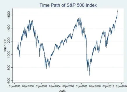
We will also divide the option data into different markets according to the time path of the S&P 500 Index. Figure 1.1 shows the time path of the S&P 3 _{http://www.optionmetrics.com/}

(18)

500 Index (daily data), daily return on the Index, and the squared daily return (volatility), from Jan 2000 to Oct 2009.

60 080 0 10 0012 0014 0016 00 S& P 50 0 In de x Date 09oct2007 31dec2002 Date 6. 66. 877 .27 .4 S& P 50 0 In de x (lo ga rit hm ) 09oct2007 Date 31dec2002 Date 0.0 05. 01. 01 5 D ai ly R et ur n S qu ar ed Date _09oct2007 31dec2002 Date

Figure 1.1 Time path of S&P 500 (daily data), daily return of S&P 500 and the squared daily return (volatility) of S&P 500; 1 Jan 2000 – 31 Oct 2009. In Figure 1.1, we see that between Jan 2000 and 31 Dec 2002, the S&P 500 index has a tendency to move downwards. Between Jan 2003 and Oct 2007, it appears to rise steadily. Between Oct 2007 and Oct 2009 (the period including the financial crisis) the volatility appears to rise markedly. This is clearly verified in the third graph (squared daily return) which represents the volatility of the S&P 500 index. Based on these observations, the option data set will be divided into three time periods: (i) “Bear Market”: 1 Jan 2000 to 31 Dec 2002; (ii) “Calm Market”: 1 Jan 2003 to 09 Oct 2007; (iii) “Crash Market”: 10 Oct 2007 to 31 Oct 2009. Sample characteristics for the data set are reported in Table 1.1.

Bear Market Calm Market Crash Market ALL Short term options: < 60 days

Implied volatility 0.26 (0.23) (0.14)0.17 (0.28)0.34 (0.22)0.26 Price 36.90 (35.43) (28.34)20.16 (37.82)33.71 (33.86)30.26 Volume 873 (769) (1610)2166 (4694)2336 (2358)1792 Observations 25,025 (19,639) (40,139)53,506 (34,987)45,613 (94,765)124,144 Medium term options: 60-180 days

(19)

(0.21) (0.14) (0.25) (0.20) Price 51.54 (41.37) (36.73)29.03 (42.21)53.23 (40.10)44.60 Volume 477 (427) 1190(924) (1274)1739 (875)1135 Observations 17,042 (13,545) (23,332)33,222 (20,227)23,359 (57,104)73,623 Long term options: > 180 days

Implied Volatility 0.24 (0.20) (0.14)0.19 (0.24)0.30 (0.19)0.24 Price 73.24 (54.01) (49.28)41.01 (59.29)78.06 (54.19)64.10 Volume 234 (273) (463)767 (762)1106 (499)702 Observations 4,254 (3,326) (6,626)9,227 (3,827)4,369 (13,779)17,850 All 46,303 (36,510) (70,097)95,955 (59,041)73,341 (165,648)215,617 Table 1.1 Sample descriptive statistics by time period and time to expiry

The table is divided into three blocks: short term (τ<60 days); medium term (60<τ<180 days); long term (τ>180 days).In each cell, the first number relates to put options, and the number below in parentheses relates to call options.The first row in each block contains average values of Black-Scholes implied volatility; the second row contains the average values of price (midpoint of bid-ask spread); the third row contains the average option volume; the last row contains the number of observations (i.e. number of options).

1.4 Literature Review

The purpose of this section is to provide a concise survey of the literature that is central to the themes of the thesis. The most important of these references will be cited again in later chapters.

Texts and general references

There is a huge number of textbooks on option theory, and they are often very similar to each other in content. One that is very popular, probably because it is comprehensive and well written, is Hull (2011). Another that we will refer to later is Adams et al. (2003). There is also a huge number of journal articles on option theory. Key references on the Black-Scholes framework for the valuation of options are Black and Scholes (1973) and Merton (1973). The key reference on the binomial-tree valuation method is Cox et al. (1979). One financial econometrics text that covers empirical analysis of option prices is Brooks (2014).

(20)

Hutchinson et al. (1994) used nonparametric methods to price European Options. The particular techniques used come under the heading of learning networks. The data is allowed to determine both the dynamics of the underlying and its relation to the option prices with minimal assumptions on either. The shortcomings of the approach is that it relies on large amount of historical prices, and therefore would not be useful for the analysis of thinly traded options.

Ait-Sahalia and Lo (1997) proposed a more advanced nonparametric kernel regression model to estimate the option price with no parametric restrictions on either the underlying asset's price dynamics or on the distribution assumed for the risk-neutral density. Ait-Sahalia and Duarte (2003) used a nonparametric option pricing model under shape restrictions to estimate the risk-neutral density. It was based on Mammen (1991)’s kernel regression model.

A more recent work related to the “model-free” regression is Pandher (2007). He presented a simple empirical approach to modelling and forecasting market option prices using localized option regression (LOR). He considered two classes of localized option regressions: structural and reduced form models. The model locally projects derivative prices on the state process of the underlying asset price, strike price, implied volatility and risk-free interest rate. The state space includes linear, quadratic and interaction terms arising among the variables. Both in-sample and out-of-sample test results showed that LOR is a relatively good model to price the options. To our best of our knowledge, it is the most closely related paper to the regression models we use in Chapter 3. Although the LOR is a good model for predicting option prices, it has limitations. In the LOR model, Pandher (2007) used implied volatility as an explanatory variable to explain option price. This seems to be a strange approach, because implied volatility is obtained directly from option price. Our regression models in Chapter 3 use historical volatility instead of implied volatility.

Andreou et al. (2008) consider non-parametric (Artificial Neural Network, ANN) and semi-parametric (CS, Corrado and Su, 1996) option pricing models, and compare these to the parametric model (BS). They use both historical and implied volatility as predictors; for historical volatility they use the past 60 days. They find that the Black-Scholes-based hybrid ANN models outperform (in predictive performance) the standard neural networks and the parametric ones.

Additive Models

Additive models (which will be used extensively in Chapter 3) were introduced by Stone (1985) and are explained in more simple terms by

(21)

Hastie and Tibshirani (1990). The components of the additive model will be obtained using B-splines, which are covered by de Boor (1987). A scatterplot smoothing technique which will be used repeatedly is the locally weighted scatterplot smoother (Lowess) due to Cleveland et al. (1979).

Implied Volatility functions and Practitioner’s Black-Scholes (PBS)

Dumas at al. (DFW, 1998) considered the deterministic volatility function (DVF) option pricing model, which assumes that volatility is a deterministic function of asset price and time. They find that this approach is no better than a simple procedure that smooths Black-Scholes implied volatilities across strike price and time to expiry. They refer to this simpler technique as the Ad-hoc model. The Ad-hoc model has since become very popular and is commonly known as the Practitioner Black Scholes (PBS) model. The PBS has become a benchmark for model comparisons in the literature. Aït-Sahalia and Lo (1998) apply non-parametric regression methods (in the form of Kernel regression) to the problem of estimating the implied volatility surface. Most other authors have used linear regression for this purpose.

Christoffersen and Jacobs (2004) consider the important question of which loss function should be used when estimating and evaluating option valuation models. They emphasise the importance of using the same estimation loss function for all models, and of using the same loss function for evaluation as for estimation. They also suggest that the choice of loss function should be guided by the objective of the exercise: that is, whether the objective is e.g. speculating, hedging or market-making. They illustrate the importance of the loss function in an application of the Practitioner Black-Scholes (PBS) model. Typically, the PBS is implemented using an implied volatility loss function, but evaluated using a pricing loss function. They demonstrate that the PBS performs much better when it is implemented using the same loss function as used for evaluation.

Christoffersen and Jacobs (2004, p.298), make a very important point when outlining the PBS procedure: “simply plugging [fitted implied volatility] into the Black-Scholes formula will yield a biased estimate of the observed call price”. However they go ahead and do exactly this. Others who use PBS appear to do the same. This motivates us to apply the smearing technique (Duan, 1983) to correct this bias. We will do this in Chapter 3.

Berkowitz (2010) takes a close look at the PBS, which he refers to as the “ad-hoc Black-Scholes method”. He shows that the PBS procedure can be used to provide an arbitrarily accurate approximation to the true option

(22)

pricing formula, at a given point in time, given a polynomial of sufficient order, and a sufficiently large sample. The approximation cannot be expected to hold over time, and because of this he recommends frequent re-calibration of the volatility surface, which produces continually new approximations. He uses simulations to examine the importance of the sample size, the order of the polynomial, and the recalibration frequency. He finds that: (1) The best performing models require only linear and quadratic terms (although it seems strange that he includes an interaction variable K*T in the quadratic model but not in the cubic model); (2) A sample size of 64 options at each time-point in time is sufficient to generate reasonable pricing accuracy; (3) Frequent recalibration is more important than the correctness of the model.

Hull and Suo (2003) find that the PBS approach based on European options does not necessarily price other types of options accurately (e.g. American Options). They define “model risk” as the risk arising from the use of an inadequate model.

Andreou et al. (2014) consider a number of regression-based implied volatility models. They consider symmetric and asymmetric models. Asymmetric means assuming the function is different for ITM and OTM options. Asymmetric models estimated separately for calls and puts are found to provide the best in-sample performance. Symmetric models using the log of the strike price are found to provide the best out-of-sample performance.

Stochastic volatility models, jump-diffusion, and the GARCH family

Bates (1991) investigates whether option prices over the period 1985-7 contained evidence of expectations of the October 1987 crash. He finds evidence of this, both in over-pricing of OTM put options, and in the jump-diffusion parameters, which indicated that implicit distributions were negatively skewed over a period which included the crash. Bates (1996) develops an efficient method for pricing American options on a stochastic volatility/jump-diffusion process. He finds that the volatility smile is explained by “jump fears”.

Bakshi et al. (1997) develop an option pricing model, named SVSI-J, that allows volatility, interest rates, and jumps all to be stochastic. They claim that the pricing formula is closed form, although one of the equations (equation (9) in the article) contains an integral so it does not seem to be “closed-form”. The model contains standard models as special cases, including Black-Scholes (BS), stochastic interest rate (SI), and stochastic volatility (SV), and stochastic volatility random-jump models (SV-J). The SVSI-J model is evaluated in comparison to the other models on three

(23)

different criteria: consistency of implied volatility with relevant time series data; out-of-sample pricing accuracy (based on predicted price of each option using the previous day’s implied parameters and implied volatility); hedging performance (where optimal hedges are obtained using the current implied parameters, and then the hedges are liquidated after one day or five days). They consider pricing accuracy to reflect a modelsstatic performance, while hedging accuracy reflects dynamic performance. The overall finding is that the modelling of stochastic volatility is much more important than that of interest rates and jumps.

Heston and Nandi (2000) claim to develop a closed-form option valuation formula for the situation in which the underlying follows a GARCH process. However, this claim is confusing because the formula is presented in Equation (11) of the article and this formula involves an integral which can only be evaluated using a numerical procedure. Hence the formula is not “closed-form”.

“Implied” GARCH parameters have been estimated using option prices by Engle and Mustafa (1992).

Duan et al. (2006) use the Edgeworth expansion to derive analytical approximations for the pricing of European options in the GARCH

framework, including GJR-GARCH (TGARCH) and EGARCH. The

approximation is essentially the Black-Scholes formula with two additional terms, one for the skewness and one for the kurtosis of the cumulative

return on the underlying. They assess the performance of the

approximation on a “test pool” of randomly generated options. They compare the approximation to the Monte Carlo value using RMSE. They find evidence that their approximation is adequate for shorter-maturity options.

The three varying volatility models we will use in Chapters 4 and 5 are ARCH (Engle, 1982), GARCH (Bollerslev et al., 1986) and TARCH (Zakoian, 1993; Glosten et al., 1993).

Monte Carlo Methods

The Monte Carlo method applied to the problem of option valuation has been discussed by Glasserman (2003) and Fink & Fink (2006). However, the method has mainly been used for options for which closed-form valuations are not available, for example American options. The studies usually rely on the standard assumption of a geometric Brownian motion process with constant return volatility.

Some studies go further and apply the Monte Carlo method to situations of varying volatility, for example Duan et al. (2006). However, that study

(24)

applies the method to randomly generated options. To our knowledge, the Monte Carlo method has not been used to value real market options under assumptions of varying volatility. This task is undertaken in Chapter 5 of this thesis.

Chapter 2 Overview of Existing Option Valuation

Methods

There are a number of established methods for option valuation.The main purpose of this chapter is to survey these methods, and to focus on the two most popular, namely the binomial-tree method, and the Black-Scholes method. The relationship between these two methods is discussed, and it is demonstrated using a specific example that they can give the same valuation under some circumstances.

It is particularly important to describe the Black-Scholes method in some detail because it is used as a benchmark for comparison when we evaluate the methods of option valuation developed in later chapters. Our discussion of the Black-Scholes method includes a heuristic derivation of the Black-Scholes formula for a European call option.

We start by introducing definitions and notation.This material is thoroughly covered in Financial Mathematics textbooks such as Hull (2011). However the notation chosen here sometimes differs from Hull (2011).

2.1 Definitions and notation

A(European) Call Optionis a security that gives its owner the right, but not the obligation, topurchase a specified asset for a specified price, known as the strike price or exercise price, at some date in the future (the expiry date).

A(European) Put Option is a security that gives its owner the right, but not the obligation, tosell a specified asset for a specified price, known as the

strike priceorexercise price, at some date in the future (expiry).

We will refer to the asset on which the option is written as theunderlying. The owner, orholder, of an option – who is said to adopt a longposition – acquires the option by paying theoption priceto thewriter– who is said to adopt ashortposition. If theholderof acall optionchooses toexercisethe

option, he pays the strike price to thewriter in exchange for the asset, at expiry. If the holder of a put option chooses to exercise the option, he delivers the asset to the writer at expiry, who simultaneously pays the

(25)

European Options can only be exercised on the expiry date.American options, in contrast, can be exercised at any time up to theexpiry date. In this thesis, we are mainly interested inEuropean Optionsbecause they are more straightforward to analyse.

Options that expire unexercised are said todie, and are worthless. The following notation will be used:

tis the current date

Tis the expiry date

_{= T – t}_{is the time to expiry.}

Stis the current (underlying) stock price.

STis the stock price at expiry.

Kis the strike price.

ris the risk-free rate of interest.

ctis the current price (or the current value) of a Call Option

ptis the current price (or the current value) of a Put Option

If you are the holder of a call option, you want the stock price at expiry to exceed the strike price.Then, you exercise the option to buy at the strike price, and immediately sell at a profit ST - K.If the stock price at expiry is

less than the strike price, you let the option die, and your payoff is zero. The payoff from holding a call option is therefore:







max 0,S K_T

Payoff diagrams are graphs showing the payoff from holding an option against the stock price at expiry,ST. Figure 2.1 shows the payoff diagram

(26)

Figure 2.1 Payoff diagram for a Call Option with strike K

A call option for which the current priceStisabovethe strike priceKis said

to be in the money (ITM). A call option for which the current price St is

belowthe strike priceKis said to beout ofthe money (OTM). A call option for which the current price St equals the strike price K is said to be at the

money (ATM).

Moneyness (for a call option) is defined as the ratio of the current price to the strike price:m = St/ K.

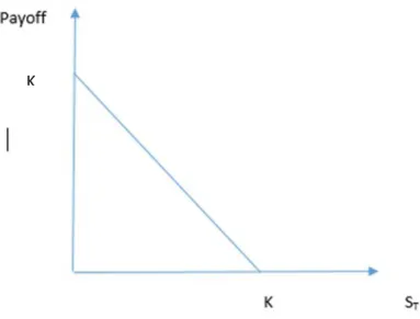
The payoff from holding a Put Option is :max 0,



K S T



Figure2.2 shows the payoff diagram for a Put Option with strikeK.

Figure 2.2 Payoff diagram for a put option with strikeK

One difference of put options from call options is that the payoff from holding a put option cannot be above K, while the payoff from holding a call is unlimited.

(27)

Moneyness for a put option ism = K /St.

The sign of moneyness (for both types of option) tells us whether the option is ITM (m>1), ATM (m=1), or OTM (m<1).

Finally, thecurrent valueof a call option is the expected value of the payoff at expiry, at the risk-free interest rate:











exp  _max 0,  _

t T

c r E S K

And thecurrent valueof a put option is the expected value of the payoff at expiry, discounted at the risk-free interest rate:











exp  _max 0,  _

t T

p r E K S

In order to compute the expectations in these two formulae, we need to make an assumption about how the price of the underlyingStevolves over

time. One such assumption gives rise to the binomial formula; another assumption gives the Black-Scholes formula. These formulae are derived in the following sections.

2.2 Binomial Tree Model

Probably the simplest technique for valuing an option is based on the construction of a binomial tree. A binomial tree is a simple method for modelling the behaviour of the underlying stock price or stock index. It simply assumes that in any discrete time period, the stock price has a fixed probability of going up by a fixed proportion, and a fixed probability of going down by a fixed proportion. We will refer to this sort of process as a “simple random walk”. The simple random walk is a discrete time version of geometric Brownian motion.

The number of steps in the binomial tree is set, and then the probability distribution of the price at expiry can be computed, and hence the value of an option can be computed. The Binomial tree method can be used to value both European and American options. In this section, we will take a close look at the method, and explain how it can be used to value European options.

We will again denote current stock price as St. First of all, we will assume

only two steps in the binomial tree; then we will consider trees with more than two steps; finally, we will demonstrate the very useful “online binomial tree calculator” in the valuation of European options.

(28)

2.2.1 Two-step binomial tree

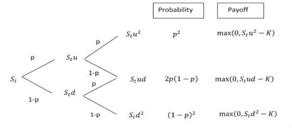
Figure 2.3 A two-step Binomial Tree

Figure 2.3 shows a two-step binomial tree that could be used to value a European call option with strikeK. The current price of the underlying isSt.

The time to expiry is divided into two periods of length/2. In each period, the stock price is assumed either to rise by a multiple u (u>1) with probability p, or decrease by a multipled (d<1)with probability(1-p). The possible pay-offs at expiry are shown in the final column of Figure 2.3, and the corresponding probabilities are shown in the penultimate column.

2.2.2 Calculation of the value of a European option using the

binomial tree

The value of an optionis the expected payoffat expiry, discounted using the risk-free rate. For the call option used as an example in Section 2.2.1, the value is:































 _         _  2 2 2 2 max 0, max 0, 2 1 max 0, 1 exp t t t c S u K p S ud K p p S d K p r

If the option was instead a put option with strike K, the value of the option would be:































  _         _  2 2 2 2 max 0, max 0, 2 1 max 0, 1 exp t t t p K S d p K S ud p p K S d p r

(29)

If the time to expiry is divided into more than two steps, the method for calculating the option value would be the same as above but the formulae would contain more terms.

The above option values are functions of u, d, and p. However, it is possible to write the formulae withoutp. This is because the value ofpcan be deduced fromuandd. This is demonstrated in the next sub-section.

2.2.3 Calculation of the probability and volatility

2.2.3.1 Calculation of probability of “up”

Consider the one-step binomial tree shown in Figure2.4.

Figure 2.4 A one-step Binomial Tree

If we assume risk-neutrality, and no-arbitrage, it must be the case that the expected price of the underlying at expiry must be equal to the value of the investment resulting from investing St at the risk-free rate between t and

expiry. In other words:



S u pt 



_S dt  



1 p



_ St exp

 

r It follows that:









  exp r d p u d (2.1)

(2.1) shows how the “up” probabilitypcan be deduced from knowledge of

uandd.

In practice, the values ofuanddare not known. They need to be deduced from the annual volatility  which is usually known. This issue is considered in the next sub-section.

(30)

2.2.3.2 Relationship between binomial-tree volatility parameters and annual volatility parameter

Consider the stock return measured as the proportion by which the stock price changes between tand t



. This is

S S

t t . The variance of this

return is given by:

 _{ }         2 t S V t S

In the two-step binomial tree model used in the last sub-section, this variance is:









               _ _              _ _        2 2 2 2 2 t S V t t 1 1 t t t S S E E pu p d pu p d S S S

The tree’s parameters should match the volatility of stock price, hence we have:









 

  _   _2 

2 ₁ 2 ₁ 2

pu p d pu p d _(2.2)

Substituting equation (2.1) into (2.2), we have:

 



 



 



 



 





 











 





_

 

_

 

_





 



2 2 2 2

exp

*

r

d

u

r

d

u

r

u

d

u

d

u d

Then we have:

 

               _    _   2 2 2 2 2 2 1 _{* exp} _* _exp _* 1 _{* exp} _* _exp _* r u du ud r d u d r u du ud r d u d Then we get:







_

  

 



 _







 

     2 ₂ 1 1 * u d * exp r * u d ud * u d * exp r u d u d Then we have:

  

 



 

 

       exp r * u d ud exp r 2 2 Finally we have:





 _{  } 2 _

_{ }

2 r r e u d ud e Using Taylor’s series expansion, we have:

(31)

   



;



u e

d e

(2.3)

(2.3) shows how the tree’s volatility parameters (uandd) can be deduced from knowledge of the annual volatilityand the time to expiry.

2.2.3.3 General binomial-tree option price formula Consider a tree with n steps.

Over the first time interval:

t t n S _ S u with probability p  



1



t t n S_ S d with probability p

Over the first two intervals:

2 2 2 t t n S_  S u with probability p





2 2 2 t 1 t n S_  S d with probability p





2 t k n k 2 1 t n S_  S u d  with probability p p

After n intervals, expiry is reached, since

S S

T



t.

The distribution of the stock price at expiry is given by:



1



n k, 0, ,

k n k k

T t n k

S _S u d  with probability C p _p  k_ _ n

The values of a call option and a put option are given by:













0 max 0, 1 exp n _{n k} k n k k t t n k k c S u d  K C p p  r    _   _  

















0 max 0, 1 exp n n k k n k k t t n k k p K S u d  C p p  r    _   _  





2.2.4 Online binomial tree calculators

If there are only a few steps in the tree, it is easy to apply the above method in order to value an option. If there are many steps, say 100, it becomes hard to apply the above method manually. However we can use an on-line “binomial tree calculator”. The original Cox, Ross, & Rubinstein (1979) tree is a popular example. This calculator returns the value of a European or American option for given parameter values, and also

(32)

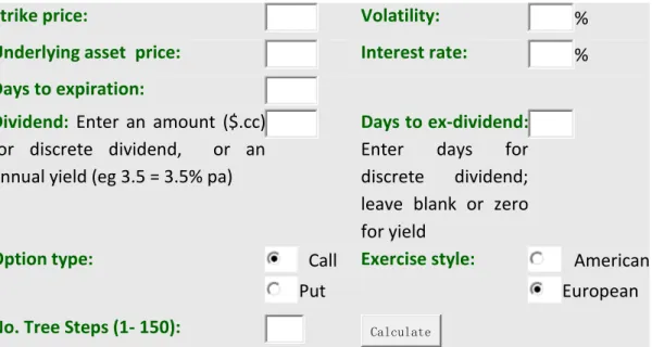
provides a graphical display of the tree structure used in the calculations. A screenshot of the input window is shown in Figure 2.5.

The user inputs numbers into the boxes (strike price, volatility, underlying asset price, interest rate, days to expiry, dividend, number of tree steps), selects the option type and exercise type, then clicks on “calculate”. One limitation of this on-line calculator is that a single user is not permitted to use it (for free) more than six times in a single day.

Strike price: Volatility: %

Underlying asset price: Interest rate: %

Days to expiration:

Dividend: Enter an amount ($.cc) for discrete dividend, or an annual yield (eg 3.5 = 3.5% pa)

Days to ex-dividend: Enter days for discrete dividend; leave blank or zero for yield

Option type: Call

Put

Exercise style: American European No. Tree Steps (1- 150): Calculate

Source: http://www.hoadley.net/options/binomialtree.aspx?tree=B

Figure 2.5 Binomial Tree on-line Calculator

Let us take as a real example a European call option traded on 14th _Jan 2002 written on the S&P 500 Index, with strike 1075 and 44 days to expiry. On 14th _{Jan 2002, the current underlying Index is 1138, the risk-free} interest rate is 0.0213, and the volatility (based on the 60-day standard deviation of returns) is 0.1605. Since we are dealing with an Index and not a single stock, the dividend is 0.

When inputting the above numbers into the online calculator, the resulting numbers are too large to appear on the screen. For this reason, we divide the price variables by 10 before inputting them. Hence, we are considering a current price of St=113.8 and a strike of 107.5.

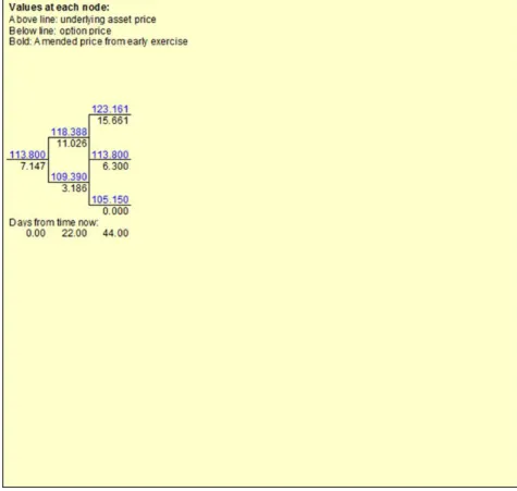
We start with 2 steps, then we extend to 10 steps, 50 steps, 100 steps and 150 steps. Figure 2.6 shows us the calculation result with 2 steps. Figure 2.7 shows us the calculation result with 10 steps. If we use the on-line calculator, the maximum number of steps that can be shown on the screen is 10.

(33)

Figure 2.6 Binomial Tree on-line Calculator Result with 2 steps

Figure 2.7 Binomial Tree on-line Calculator Result with 10 steps From Figure 2.6, we see that the value of this European call option with 2 steps is 7.15; from Figure 2.7, we see that the result with 10 steps is slightly lower at 7.05. Remember that we divided the underlying stock price and

(34)

the strike price by 10, so if we convert to the original units, the option value with 2 steps is 71.5 and with 10 steps 70.5. Does the binomial tree online calculator give the same result as the formula derived in section 2.2.3? Let us check this. The information we have about the option is shown in Table 2.1.

St K rf  

1138 1075 2.13% 44 days 16.05%

Table 2.1 Information for the Option Example

Following the stages of the binomial tree calculationas discussed in section 2.2.3, we first need to calculate the values of u and d. According to equation 2.3, we have:

‴ ‴ ‴

d ‴ ‴ ‴

Secondly, we need to distribute a two-step binomial tree.

1138 1184 1094 1231 1138 1052 156 63 0 payoff

Figure 2.8 A two-step Binomial Tree example Finally, we calculate the value of call option:



156*0.25 63*0.5 0*0.25 *exp 0.0213*



44 70.5 360

 

  _ _

 

When we use the formula to calculate the same European call option, we find the value is $70.5 which is close to the result from online calculator. We will use the same calculator to calculate the value of the European call option with 10 steps, 50 steps, and 100 steps. The results are shown in Table 2.2. We see that the call value falls when the number of steps rises, but it seems to be converging to a value around 70.2.

(35)

steps 2 10 50 100

Call Value 71.5 70.5 70.3 70.2

Table 2.2Binomial Tree on-line Calculator Result Results with different numbers of tree-steps

One major advantage of the binomial model is that it can be used to value American Options. This is because with the binomial model, it is possible to check at every node of the tree for the profitability of early exercise. When a node is found to have profitable early exercise, the part of the tree coming off that node is removed and replaced with the intrinsic value at that point. A limitation is that the speed of calculation is relatively slow. It is not a practical approach for the calculation of thousands of prices in a few seconds.

2.2.5 Binomial Tree with TGARCH Effect

In Sections 2.2.1-2.2.4, we discussed the binomial tree on the basis of the assumption of a simple random walk. However, later in the thesis, we use the TGARCH model to predict the option price. The TGARCH model (Threshold ARCH, or “GJR-GARCH”, Glosten et al., 1993) is a model that allows the effects of good and bad news to have different effects on volatility. A feature of stock prices is that “bad” news tends to have a larger effect on volatility than “good” news. The tendency for volatility to fall when price rises and to rise when price falls is known as the “leverage effect” (Enders, 2004). In this section, we consider whether the assumption of a TGARCH volatility process instead of a simple random walk, in the context of a binomial tree, changes the valuation of some options. We will use a 2-step binomial tree model.

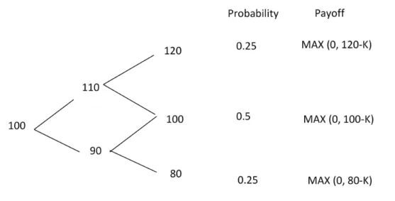
We assume that time to expiry is one year, and the year is divided into two 6-month steps. We first assume a simple random walk: the current stock price is 100, and at each step the stock price either rises by amount 10 with probability 50%, or falls by amount 10 probability 50%. The risk-free interest rate is 5%. The following diagram illustrates the tree.

(36)

Figure 2.9 (a) A two-step binomial tree with simple random walk assumption

Consider two call options: an OTM call with strike K=110, and an ITM call with strike K=90. The values of these two options are computed to be:









    ( 110): 10*0.25 *exp 0.05*1 2.38 OTMcall K c









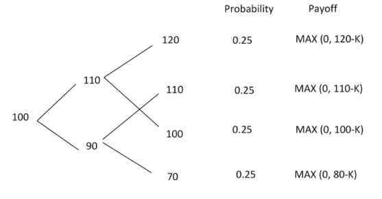
    ( 90): 30*0.25 10*0.5 *exp 0.05*1 11.89 ITMcall K

Next we assume that the stock price process follows a TGARCH process. We assume that if the price rises in the first step, the second step is the same as for the simple random walk. However, if the price falls in the first step, volatility in the second step doubles, and the price changes by 20 instead of 10. This gives the following tree.

(37)

Figure 2.10 (b) A two-step binomial tree with TGARCH assumption Under the TGARCH assumption, the values of the two call options are:









    ( 110): 10*0.25 *exp 0.05*1 2.38 OTMcall K c









     ( 90): 30*0.25 20*0.25 10*0.25 *exp 0.05*1 14.27 ITMcall K

We see that the value of the OTM call is unaffected by the TGARCH assumption. However, the value of the ITM call is around 20% higher under the TGARCH assumption.

Next, we consider put options. If the stock price follows a simple random walk, let us consider two put options: an OTM put with strike K=110, and an ITM put with strike K=90. The values of these two options are computed to be:



90 :





10 * 0.25 exp 0.05 * 1







2.38 OTM put K  p   K 110:p10*0.530 *0.25exp0.05*111.89 put ITM

Under the TGARCH assumption, the values of the two put options are: K 90: p20*0.25exp0.05*14.75 put OTM



K  110



:p 



10 *0.25  40 *0.25



exp



0.05 *1



11 .89 put ITM

We see that the value of the ITM put is unaffected by the TGARCH assumption. However, the value of the OTM put is around 50% higher under the TGARCH assumption.

(38)

In Chapter 4, we find strong evidence of a TGARCH process in daily stock index data. This means that, by the above analysis, ITM call options and OTM put options are likely to appear over-priced if the random walk (e.g. Black-Scholes) is assumed. This is the well-known “volatility smirk” that is indeed seen in option price data: ITM calls tend to have higher implied volatilities than OTM calls, and OTM puts tend to be higher implied volatilities than ITM puts, which is equivalent to saying that they are over-priced under Black-Scholes assumptions. The simple analysis in this section is proposing a simple explanation for the volatility smirk and table 2.3 gives us a summary of the results.

ITM Call OTM Call ITM Put OTM Put

Simple Random

Walk 11.89 2.38 11.89 2.38

TGARCH 14.27 2.38 11.89 4.75

Table 2.3 comparison results of simple random walk with TGARCH

2.3 The Black-Scholes Method

2.3.1 Heuristic derivation of Black-Scholes formula

The Black-Scholes formula is considered as the most prominent achievement in option pricing theory. The formula is used to calculate the theoretical European Option price (ignoring dividends paid during the life of the option) using the five key determinants: price of underlying, strike price, volatility, time to expiry and risk-free interest rate.

Most textbooks use differential calculus and Ito’s lemma to derive the Scholes valuation formula. In this section, we will derive the Black-Scholes valuation formula, using the “heuristic derivation”, presented by Adams et al. (2003). This method is more straightforward since all that is required is a formula for the truncated mean of the lognormal distribution. We will start the derivation the Black-Scholes formula by listing its assumptions. The Black-Scholes formula is based on 7 important assumptions:

(1) Stock Returns are normally distributed with known mean and variance; (2) The annual volatility is constant;

(3) No arbitrage argument;

(4) The risk-free interest rate on the money market is known and constant; (5) No trading cost;

Flexible Option Valuation Methods