Groupe de Recherche en Économie et Développement International
Cahier de recherche / Working Paper
09-03
Professional Liability Insurance Contracts: Claims Made Versus
Occurrence Policies
M. Martin Boyer
Professional Liability Insurance Contracts: Claims Made Versus
Occurrence Policies
∗
M. Martin Boyer
†and Karine Gobert
‡December 15, 2008
Abstract
One of the major contract innovation in liability insurance during the liability crisis of the early 1980s was the introduction of claims-made and reported insurance contracts. Typical insurance contracts are based on loss occurrence (i.e., occurrence-based contracts), which means that a loss incurred in a given year is covered by the insurance contract for that year, no matter when the claims is actually reported.
In a claims-made contract, losses are covered in the year in which they are reported. The major difference
between the two types of contract is thus that occurrence contracts are forward looking whereas
claims-made contracts are retrospective. The goal of this paper is to analyze the efficiency of both forms of
insurance contract and the reasons why policyholders would prefer one contract over the other.
JEL Classification: G22, D86.
Keywords: Liability insurance, Claims-made and reported, Loss development, Income smoothing.
∗This research isfinancially supported by the Fonds pour la Formation des Chercheurs et d’Aide à la Recherche (FCAR -Québec) and by the Social Science and Humanities Research Council (SSHRC - Canada). The continuing support of Cirano
is also gratefully acknowledged.
†CEFA Professor of Finance and Insurance, HEC Montréal (Université de Montréal); 3000, chemin de la
Côte-Sainte-Catherine, Montréal, QC H3T 2A7 Canada; andCirano, 2020 University Ave., 25thfloor, Montréal, QC. martin.boyer@hec.ca
‡Faculté d’administration and GREDI, Université de Sherbrooke; andCirano, Montréal, QC. Tel (819) 821-8000 ext. 62315,
Professional Liability Insurance Contracts:
Claims Made Versus Occurrence Policies
Abstract: One of the major contract innovation in liability insurance during the liability crisis of the early 1980s was the introduction of claims-made and reported insurance contracts. Typical insurance contracts are based on loss occurrence (i.e., occurrence-based contracts), which means that a loss incurred in a given year is covered by the insurance contract for that year, no matter when the claims is actually reported. In a claims-made contract, losses are covered in the year in which they are reported. The major difference between the two types of contract is thus that occurrence contracts are forward looking whereas claims-made contracts are retrospective. The goal of this paper is to analyze the efficiency of both forms of insurance contract and the reasons why policyholders would prefer one contract over the other.
Keywords: Liability insurance, Claims-made and reported, Loss development, Income smoothing.
1
Introduction
The liability crisis of the late 1970s and early 1980s was a period of intense uncertainty for insurance companies. This crisis affected all types of liability insurance including personal automobile liability insurance (see Cummins and Tennyson, 1992), medical malpractice (see Nye and Hofflander, 1987), product liability and general liability (see Berger, Cummins and Tennyson, 1992). Doherty (1991) attributed this uncertainty to changes in the legal environment. As changes in the legal environment was an undiversifiable risk for insurers, the law of large numbers no longer applied completely to these insurance products, so that premiums needed to be increased to cover legal environment risk. Doherty (1991) concludes that the increased economic importance of mutual insurance companies resulted directly from this liability crisis. This organizational response of the insurance industry was also accompanied by a contractual response: The introduction of claims made and reported (CMR hereafter) insurance policies. These contracts contrast with the traditional occurrence-based insurance contract (OB hereafter). In an OB contract, a policyholder is insured for losses that are incurred during the insurance policy year even if the loss is not reported for many more years. CMR insurance contract on the other hand insure policyholders for losses that are reported during the policy year even if the loss was incurred many years before (subject to a retrospective date or time limit). The apparent dominance of claims-made policy was such that even St. Paul Fire and Marine, a major medical malpractice insurer in the 1980s, switched its entire medical malpractice book of business to claims-made around that time. By 1984, CMR policies accounted for fifty percent of total premiums written in medical malpractice, and Posner (1986) anticipated that CMR policies would account for seventy to eighty percent of the medical malpractice insurance premium earned during 1985. Today, approximately 75% of medical malpractice insurance is being sold under a claims-made approach. CMR policies gained favor not only in the medical malpractice and professional liability arena, but also for some type of general liability and product liability protection (Sloan, Bovjberg and Githens, 1991).
The paper focuses on the difference in the policyholder’s expected utility from each contract type. An underlying assumption we shall use is that the insurance market is competitive so that the premium paid is equal to each policyholder’s expected loss. As a result, we are able to concentrate on the impact of the contract structure’s differences rather than insurer profitability.
To better understand how the two types of contracts work, we concentrate on three features of the contracts: The way losses develop over the years, how insurance premiums are calculated, and the impact of risk aversion on the decision to purchase one contract or the other. Our paper presents two main results.
First, we show that when everyone in the economy is risk neutral, then the only reason why insured agents would prefer the CMR contract is that the discount factor they apply to future cash flows is lower than the insurer’s, which means that the present value of future cash flows is worth less to the agent than to the insurer. This result holds true whether we allow undiversifiable shocks to impact losses or the claim over time. Our second main result is that when insured agents are risk averse, then they are more likely to prefer the CMR contract over the OB contract when the tail of the loss is longer. This means that for short-tail lines, such as automobile and homeowner insurance, claims-made and reported insurance contracts do not dominate as much traditional occurrence based contracts than in long-tail lines such as medical and professional malpractice liability insurance.
Our theoretical model corresponds to many data regularities we observe in property and casualty insur-ance. Let us think of the facts that OB contracts are more popular in short-tail personal lines and that CMR contracts are popular in long-tail liability lines where the insured agent is more likely to be risk averse (i.e., medical malpractice insurance). This contrasts with the theory developed by Doherty (1991) which suggests that claims-made contracts are an answer to an increase in the uncertainty of the legal environment in which insurers operate. Although Doherty’s theory explains why claims-made contracts are more prevalent in long-tail lines, it does not explain why claims-made contracts are more prevalent in personal liability lines when, in fact, risk averse individuals should be more reluctant to assume the legal environment uncertainty than risk neutral insurers. Our theory offers predictions that one could bring to the data, such as the fact that for risk neutral agents, CMR contracts should be preferred to OB contracts when the insured agent has important liquidity constraints so that he discounts future cash flows much more than if he were not liquidity constrained. In the same vein, Doherty and Dionne (1993) suggest that claims-made, as well as the creation of risk retention groups, were designed to reduce the impact of non-diversifiable risk on insurers.
The paper is organized as follows. We first present the economic importance of each type of insurance contract, how insured losses develop and how pure premiums should be calculated given these losses. We then present the problem that a risk neutral agent faces in an economy where there are no systematic shocks to the distribution of losses. We introduce shocks to the loss distribution in Section 4 and move to a risk averse agent in Section 5. Finally, we discuss the empirical predictions of the model that one could bring to the data and conclude in the last section of the paper.
2
Economic Importance and Model Setup
2.1
Economic importance of each contract type
Claims-made contracts are mostly popular in liability lines where the damage has been caused by an indi-vidual who exercises his profession. In particular CMR contracts are highly popular, or even the norm, is the case of medical malpractice liability insurance contracts, directors’ and officers’ liability insurance contracts and other professional liability situation where the insurance contract is designed to protect lawyers and ar-chitects in case of a professional error.1 The rising importance of CMR policies has led the NAIC to include
a separate aggregate report for lines of business where CMR policies are important starting in 1995. These lines of business are medical malpractice liability insurance, product liability insurance and other liability insurance, which include directors’ and officers’ insurance and other types of professional liability insurance. Table 1 presents total premiums earned in the United States over the past decade for the case of medical malpractice insurance as a function of the type of contract.
Table 1. Premium earned (in thousands of current dollars) in medical malpractice insurance by type of contact, 1997-2006
year Total premiums earned OB contract premiums earned CMR contract premiums earned Percentage of total in CMR contracts 1997 5,032,842 1,441,057 3,591,785 71.4% 1998 5,128,893 1,465,654 3,663,239 71.4% 1999 5,267,617 1,591,712 3,675,905 69.8% 2000 5,351,526 1,861,044 3,490,482 65.2% 2001 5,780,544 1,718,908 4,061,636 70.3% 2002 9,157,351 2,430,379 6,726,972 73.5% 2003 8,302,736 2,496,678 5,806,058 69.9% 2004 8,784,556 2,145,038 6,639,518 75.6% 2005 8,629,529 2,065,908 6,563,621 76.1% 2006 10,140,990 2,355,646 7,785,343 76.8%
Source: Born and Boyer (2008) using the National Association of Insurance Commissioners annual data tapes — Property and Casualty Insurers, Underwriting and Investment Exhibit.
Thefigures in the table include premium from all insurers reporting nonzero premiums in
either type of medical malpractice insurance policies.
As we see, the importance of claims-made contracts has risen over the years and accounts for close to 77% of the total premiums earned in the medical malpractice insurance line of business in 2006. This compares to 71% in 1997 and 70% in the early nineties according to Born and Boyer (2008). It is clear that CMR policies increased in popularity and are gaining ground amongst policyholders in the medical malpractice
1In one important American insurance company, the following profesional protections are offered on a claims-made basis:
Directors and officers liability, Private company liability, Employment practices liability, Fiduciary liability, Bankers professional liability, Insurance company liability, Security & privacy liability, and Employed lawyers professional liability.
insurance industry (see Harrington, Danzon and Epstein, 2008, for a discussion of the market for CMR and OB policies).
It is not obvious that CMR contracts have increased in popularity in other lines of business where they are available. In Panel A of Table 2 we present the total premiums earned by contract type for the medical malpractice, product liability and other liability lines of business for the years 2003 through 2006.
Table 2. Premium earned (in millions of current dollars) and number of insurers by type of contact in product liability and other liability lines of business, 2003-2006. Panel A: Earned premium
Line of business Contract 2003 2004 2005 2006
Medical malpractice OB $ 2,497 $ 2,145 $ 2,065 $ 2,356 CMR $ 5,806 $ 6,639 $ 6,564 $ 7,785 %CMR/total 69.9% 75.6% 76.1% 76.8% Product liability OB $ 2,165 $ 2,754 $ 2,936 $ 3,042 CMR $ 323 $ 391 $ 512 $ 527 %CMR/total 13.0% 12.4% 14.8% 14.8% Other liability OB $ 20,121 $ 23,698 $ 23,739 $ 26,407 CMR $ 12,323 $ 14,781 $ 15,402 $ 15,237 %CMR/total 38.0% 38.4% 39.3% 36.6%
Panel B: Number of insurers
Line of business Contract 2003 2004 2005 2006 Medical malpractice OB 269 222 223 263 CMR 332 365 354 394 Product liability OB 560 551 534 543 CMR 196 181 169 175 Other liability OB 1222 1215 1226 1252 CMR 575 584 571 577
Source: Born and Boyer (2008) and authors’ calculations using the National Association of Insurance Commissioners annual data tapes — Property and Casualty Insurers, Underwriting
and Investment Exhibit. Thefigures in the table include premium from all insurers reporting
nonzero premiums in the appropriate insurance line.
We see that the popularity of claims-made contracts has increased relative to occurrence-based contracts only in the medical malpractice area; in the two other lines where claims-made contracts are available, there does not seem to be a large movement in the contract preferences of the policyholders. Even when we look at the number of insurance companies that provide each type of contract in these three lines as in Panel B of Table 2, we do not see insurers offering CMR contract being much more numerous relative to the number of insurers offering OB contracts.
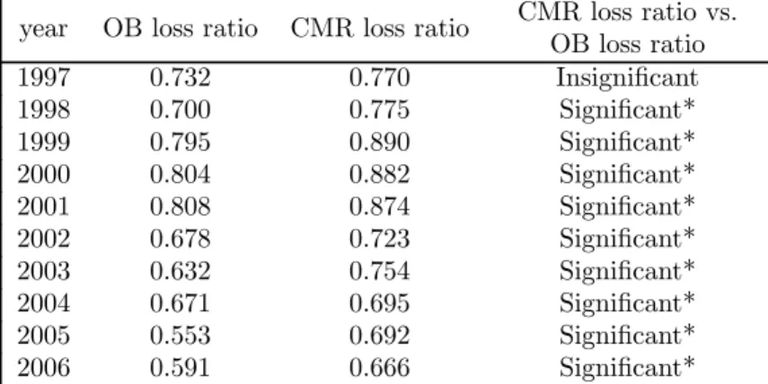
Another interesting comparison we can make between OB and CMR contracts is with respect to the loss ratio (losses incurred divided by premiums earned) for each type of contract. Table 3 presents those loss ratios by contract type for the medical malpractice insurance industry.
Table 3. Median loss ratio (losses incurred divided by premiums earned) in the medical malpractice insurance industry by type of contact, 1997-2006
year OB loss ratio CMR loss ratio CMR loss ratio vs. OB loss ratio 1997 0.732 0.770 Insignificant 1998 0.700 0.775 Significant* 1999 0.795 0.890 Significant* 2000 0.804 0.882 Significant* 2001 0.808 0.874 Significant* 2002 0.678 0.723 Significant* 2003 0.632 0.754 Significant* 2004 0.671 0.695 Significant* 2005 0.553 0.692 Significant* 2006 0.591 0.666 Significant*
Source: Born and Boyer (2008) using the National Association of Insurance Commissioners annual data tapes — Property and Casualty Insurers, Underwriting and Investment Exhibit and Schedule P, Part 2F. Table includes only insurers with positive premiums earned in each year.
Losses incurred include defense and cost containment expenses. *Significance of differences
between medians was determined through quantile regressions with bootstrapped standard errors.
It is interesting to note that the loss ratio of CMR policies have been consistently higher than the loss ratio of OB policies over the past decade, and significantly so except for the year 1997. This suggests that underwriting profitability is lower in the CMR line than in the OB line. A natural question we can ask after looking at the economic importance of OB and CMR contracts and the type of losses they are designed to cover is why there are two types of contracts that coexist in these insurance lines of business. What makes these markets attractive for both CMR and OB contracts to coexist whereas the traditional OB contract is the norm in other personal lines?
2.2
Loss development and premium
When a loss is incurred, it may take a certain number of years until it is claimed and settled. For instance, construction blocks for kids may have been mistakenly painted using lead-based paint in 1990, but not discovered before 1998. In this case the loss was incurred the year when the construction blocks were painted, but it took eight years before any claim isfiled, and even more time yet before it is settled. One can also think of medical doctors who perform operations and diagnostics on a regular basis and who may be make an error. Although the mistake is committed in 1995, it may take ten years before anyone realizes that it was made. The same is true for other types of professional risks associated with being an engineer, an architect, a nurse, or even a corporate director or officer.
Loss development refers to the proportion of claims that is paid in the years following the one where the loss was incurred. For example, suppose that historically 50 % of claims incurred in yeart are paid in year
t, 25 % in year t+ 1, 15 % in yeart+ 2 and 5 % in yearst+ 3andt+ 4. This loss is thus said to takefive year to fully develop. We could then say that the tail of the loss isfive years long.
Suppose an agent faces in period t a potential once-in-a-lifetime loss L distributed according to some functionf(·)with meanE(L) =Land varianceσ2and no other loss in any other period. The development
cycle of this loss is given byα0, ..., αn whereαi is the proportion of incurred losses that are settled in period
t+i. The number of years until the loss if fully developed isn+1. Of course we haveαi ∈[0,1),i= 0,· · ·, n,
andΣn
i=0αi= 1. DenoterI the insurer’s discount rate of future losses so that the insurer’s constant discount
factor isδI =1+1rI. Because the market is competitive, the premium must be equal to the present value of
the expected loss. The loss development pattern is given in the following table together with the implied expected cost of the loss for the period in which the loss is reported.
Table 4. Loss development for a loss incurred in periodt
Period Proportion of loss reported Period 0 value of loss L t α0 α0L t+ 1 α1 δIα1L ... ... ... t+n αn δnIαnL t+n+ 1 0 0 ... 0 0
The table presents the proportionαiof a period-t loss that are reported in each
subsequent periodt+i(so thatΣiαi= 1) and the present value, in period t,
of this reported loss using discount rateδI.
With OB policies, the individual pays in periodta premium that covers the loss incurred intregardless of the date at which the claim is reported and settled in the future. The premium paid in period t must cover all possible future payments by the insurer related to this period t’s loss. The present value of the insurer’s expected payment isPt=Σni=0δ
j
IαjE(L). In other words, the premium today must cover all losses
that will be paid in the future even though the loss is incurred today.
In the case of CMR policies, the premium that is paid today must cover losses that are paid today, no matter when such a loss was incurred, today or in the past. For a loss incurred in t, a premium must be paid in every subsequent periods in which a claim can be settled for this loss. That is, for a periodtloss, a premium is paid in periodtand in each of thensubsequent periods, until the loss is fully developed. In the first year of the CMR policy (att), only thefirst year’s reported loss needs be insured. This means that the first year’s premium is given by Pbt=α0E(L). In the second year, at time t+ 1, the premium is given by
b
the premium isPbt+2=α2E(L); and so on. At any timet+i≤t+n, the premium isPbt+i=αiE(L). It is
obvious that for an event occurring in period t, the premium the insurer receives under an OB contract is exactly equal to the discounted sum of premiums she receives under a series of CMR contracts. Indeed, the present value in period t of all the premiums paid in a CMR contract is given byΠbt =Σni=0δ
j
IPbt+i.When
substituting forPbt+i, wefindΠbt =Σni=0δ j
IαjE(L) =Pt, which it the premium paid in periodt under an
OB contract. We summarize bellow the notation we shall use throughout the paper.
Development pattern (α0, α1,· · ·, αn),Pni=0αi= 1
End period probabilities are also called thetailof the development pattern. If the late periods’αs are high compared to the early periods’,
then we say that the tail isthick. Discounting δ= 1
1+r,r is the corresponding cost of capital
Insurer and agents may have different factors denotedδI andδA respectively.
3
Risk Neutral Agents and Shockless Economy
We now suppose that a risk neutral individual lives forK periods and is exposed to some risk during the first T + 1 periods, that is, the active periods of his life. In period t ∈ [0, T] the agent faces a potential lossLt with an invariant distribution f(·) and mean E(Lt) = L. We suppose that there is no change in
loss development patterns ({αt}n0) over time and that any loss is fully developed before the individual dies,
T+ 1≤K−n.
Because the distribution and development of the loss is the same in every period, the OB premium will be the same in every period. The agent can therefore be insured with a series of OB contracts so that he pays a premiumPt in every periodtfrom 0toT and nothing thereafter so that
Pt=P = n X j=0
δjIαjL.
In the case of CMR policies, the premium that is paid today must cover losses that are paid today, no matter when such a loss was incurred. In the first year of the CMR policy (at t = 0), only first year’s reported losses need to be insured. This means that thefirst year’s premium is given byPb0=α0L. In the
second year, at timet= 1, the premium is given byPb1=α0L+α1L; thefirst term is the amount that will
be paid to cover losses that are incurred in period t= 1, whereas the second term is the amount that will be paid to cover losses that were incurred in period t= 0, but are not reported until periodt= 1. At time
for the growing number of potential past losses. In period t=n, the period 0 loss has fully developed and the premium is b Pn= n X j=0 αjL=L.
After thefirstnyears of the agent’s professional life and until the end of his career, he can buy each year a CMR contract insuring for loss reports from thenpreceding years. PremiumPbt=Pbn is then paid so long
as the individual is working, for periodst∈{n, T}.
After retirement the individual still needs to purchase insurance to cover losses that were incurred in the past, but have not been reported yet. Such an individual does not need to purchase insurance for losses that are to be incurred this year since he is no longer exposed to such losses. In periodT+ 1, his premium then starts to decrease and becomes
b Pt= n X j=t−T αjL, t=T+ 1,· · · , T+n
untilt=T+n. After that date, he no longer pays any premium (Pbt= 0for allt≥T+n+ 1).
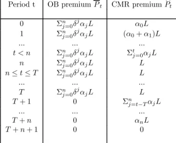
The following table presents premiums that must be paid each year for the two types of contract:
Table 5. The premiums paid using a sequence of Occurrence based (OB) insurance contracts compared to the premiums paid using a sequence of Claim made and reported (CMR) insurance contracts.
Period t OB premiumPt CMR premiumPbt
0 Σn j=0δ j αjL α0L 1 Σn j=0δjαjL (α0+α1)L ... ... ... t < n Σn j=0δ j αjL Σtj=0αjL n Σn j=0δjαjL L n≤t≤T Σn j=0δ j αjL L ... ... ... T Σn j=0δjαjL L T+ 1 0 Σn j=t−TαjL ... ... ... T+n 0 αnL T+n+ 1 0 0
Loss develops completely overnperiods, a loss may be incurred in thefirstT periods.
If individuals actualize future premiums at rate rA invariant over time so that their discount factor is
given byδA = 1+1rA, then the present value of all premiums paid over the individual’s lifetime with an OB
insurance policy is given by
Π= T X t=0 δtAP = T X t=0 δtA n X i=0 δiIαiL
In the case of a CMR insurance policy, the present value of the premiums paid is b Π= TX+n t=0 δtAPbt= n X t=0 δtA t X i=0 αiL+ T X t=n+1 δtA n X i=0 αiL+ TX+n t=T+1 δtA n X i=t−T αiL.
ComparingΠwithΠ, we can state the following proposition.b
Proposition 1 If the loss development pattern (α0, ..., αn) and the distribution of the loss do not change
over time, then risk neutral policyholders will prefer a CMR contract to an OB contract if and only ifδI > δA
(or equivalently, rI < rA).
Proof. All proofs are relegated to the Appendix.
The difference between the two profiles stands in the timing of their premiums. This timing matters for a risk neutral agent only inasmuch as different discount factors can be affected to the payments. Suppose we look at the loss that is incurred in period 0. The OB premium for this loss discounts future potential losses at the insurer’s rate: P0=Σnt=0δtIαtL. In the case of the CMR contract, the insurer receives a premium in
each period for the payment she is likely to make in the same period. The insurer’s discount rate does not influence the CMR premium whereas the agent actualizes future premiums using discount factor δA. This
means that the CMR contract cost perceived by the agent is Πb0 = Σnt=0δ t
AαtL. Therefore, an agent will
prefer the CMR contract to the OB contract if and only ifδI > δA(i.e., if and only if rI < rA).
We can infer from this proposition that if the insurer and the policyholder use the same discount rate, then the risk neutral policyholder will be indifferent between the two policies. If the interest rate used by the agents (rA) to discount future cashflows is greater then the insurer’s interest rate (rI), then the agent
will surely prefer a CMR policy to an OB policy. As a result, myopic or impatient agents prefer to purchase CMR policies. Because myopic agents value the present proportionally more than the future, they prefer to pay lower premiums in the short run even if it means paying more in the long run. This allows us to make ourfirst prediction.
Prediction 1. For losses that are not influenced by external shocks and for risk neutral policy-holders, a CMR policy will be preferred to an OB policy if and only if the insured’s cost of capital is greater than the insurer’s.
4
Shocks to the Loss Distribution
Proposition 1 assumed that the distribution of losses was invariant in time. Doherty (1991) claims, however, that it is because of the uncertainty in future losses that insurers started offering CMR policies. We explore
this possibility in this section. We introduce periodic shocks affecting the loss distribution. We must then distinguish between two cases. If the distribution of the shock is known to all so that the expected value of the shock is the same in period0as in the period where the shock occurs, there is no uncertainty on the loss distribution, only an anticipated trend is the expected loss. On the other end, if the distribution of the shock is unknown, the expected value in period 0 of the shock int, is not the same as the expected value intof the shock int. In this case, there is uncertainty on future loss distributions since shocks are unanticipated. We show that whether the shock is anticipated or not has no impact on the risk-neutral comparative evaluation of the contracts.
4.1
Anticipated shocks to the loss distribution
Let us assume that the claim paid by the insurer can evolve independently of the event because, for instance, the size of the claim is related to the regulatory environment in place at the moment the claim isfiled rather than the moment the loss is incurred. The loss distribution is the distribution of the claim regardless of the period in which the event took place. That information is known to the policyholder and the insurer. The shocks to the loss distribution are anticipated in the sense that E(Lt+i)is invariant, that is, there can be
shocks to the loss distribution but the expected value of these shocks are perfectly known from period 0 on. An OB contract signed in period t takes account of future expected claims that may arise following an event int. The OB premium, then, is forward looking:
Pt=Σni=0δiIαiE(Lt+i).
On the other hand, in a CMR contract, the premium in period t only depends on the loss claimed in periodtregardless of when in the past the event occurred. The premium writes:
b Pt= l X i=k αiE(Lt), wherek= 0, l < nift < n,k= 0, l=nifn≤t≤T andk=t−T, l=nift > T.
Premiums are no longer constant. Making a choice between CMR or OB contract in period t, an agent considers the difference in premiums. The next Proposition establishes that from periodton, only discounting can make a difference between the two types of contracts.
Proposition 2 If the distribution of loss changes over time, risk neutral policyholders will prefer a CMR contract to a OB contract if and only if δI > δA (or equivalently,rI < rA).
Suppose a single event occurring in period t. The OB premium is paid only once and covers all future claims related to this loss:
Pt=Σni=0δiIαiE(Lt+i).
The sequence of premiums that will be paid using a CMR contract to cover for the period t loss is given by
b
Pt+i=αiE(Lt+i), i= 0,· · ·, n.
In period t, the agent correctly anticipates that the CMR premium will be Pbt+i in t+i. There is, then,
no uncertainty on future premiums, neither in OB nor in CMR arrangements. The discounted sum int of future CMR premiums related to an event intis, then,
Σni=0δiAPbt+i=Σin=0δiAαiE(Lt+i).
If δI = δA, this amounts to the same. It is clear that an agent prefers a CMR arrangement only if his
discount factor is lower than the insurer’s one. With equal discount factor, a risk neutral agent is indifferent between payingPt now or anticipating to pay a sequence of premiumsPbt+i,i= 0,· · · , nthat he discounts.
As long as the distribution of the shocks is known, there is no uncertainty and the expected value of a period t loss is correctly anticipated in period 0 by both the insurer and the insured. Proof of Proposition 2 makes it obvious, once the terms are rearranged to highlight the expected discounted sums of premiums, that only the discount factors matter in comparing the two premium profiles. Accounting for the associated future loss distribution of losses does not change a risk neutral agent’s evaluation of the intertemporal value of each type of contract.
4.2
Unanticipated shocks to the loss distribution
In this subsection, we explore the case of an uncertain distribution of future losses to see if that introduces a difference between the two types of contracts. Uncertainty means that the expected value of a periodt loss is not the same if it is evaluated in periodtwith the information available in periodtas if it is evaluated in an earlier period. Put differently, we will assume that even if agents know that the expectation they have of future losses is wrong, they cannot improve it. In that case, OB premiums, that are forward looking, rely on imperfect information about future losses.
Let us denote Et(Lt+i), i= 0,· · ·, n, the expected value of a claim in t+i conditional to information
available int. Unanticipated shocks to the loss distribution imply that the distributionLtvaries from period
The OB premium for an event incurred in periodt is paid int and equal to Pt= n X i=0 δiIαiEt(Lt+i).
If the agent decides to enter a sequence of CMR contracts, he should expect to pay a sequence of premiums b
Pt+i,i= 0,· · ·, nsuch that
b
Pt+i=αiEt+i(Lt+i).
The best predictor an agent can use in periodtto evaluateEt+i(Lt+i)isEt(Et+i(Lt+i)) =Et(Lt+i). Hence,
in periodt, the policyholder’s expected discounted sum of future premiums paid in a CMR arrangement is
Et à n X i=0 δiAPbt+i ! =Et à n X i=0 δiAαiEt+i(Lt+i) ! = n X i=0 δiAαiEt(Lt+i).
Again, the discounted value of insurance evaluated int is the same in both contracts ifδA=δI.
The insurer and the insured know that the OB premium is computed with imperfect information. The OB insurer is the bearer of this error’s consequences since he is the one to pay for potential future losses the true expected value of which he does not know. A CMR contract shifts the burden of uncertainty to the insured. A CMR contract is a better way of dealing with uncertainty in the sense that it allows to wait for accurate information before premiums are computed. In standard property/casualty insurance contracts, a premium is paid each period and incorporates all new information arrived in the period. It is therefore interesting to see that OB contracts, that lock the insurer into future obligations after premiums have been paid once and for all, are still very popular amongst insurers even when insurers are faced with this type of uncertainty. This leads to us to make a second prediction.
Prediction 2. For losses that are influenced by unanticipated shocks a CMR policy should be preferred to an OB policy only because it allows to account for relevant information at the time it accrues.
5
Risk aversion
Given that OB and CMR contracts offer premiums that do not differ in present value, it follows that if insured agents discount the future at the same rate as insurers, a remaining motive for using one contract or the other must be that agents are somehow risk averse. A risk averse agent endowed with a concave utility function has a preference for the smoothing of his consumption. Since the difference between CMR and OB contracts is all about the timing of cashflows, a risk averse agent may prefer one particular contract because of this smoothing effect.
Suppose an agent has a constant wealthY per period. His consumption in periodtisY−PtwherePtis
the premium paid int to buy an insurance contract. The agent values consumption with a concave utility function u(Y −Pt) with u0 >0 and u00 <0. We assume that the distribution of losses is invariant such
that E(L) =L. The agent now compares intertemporal utilities under each contract. With OB and CMR premiums equal to Pt and Pbt respectively (see Section 3), the agent’s intertemporal utility over his entire
life is UOB= T X τ=0 δτAu à Y − n X i=0 δiIαiL ! + K X τ=T+1 δτAu(Y)
with a sequence of OB contracts. With a sequence of CMR contracts, his intertemporal utility from period 0 on is: UCM R = n X τ=0 δτAu à Y − τ X i=0 αiL ! + T X τ=n+1 δτAu(Y −L) + TX+n τ=T+1 δτAu à Y − n X i=τ−T αiL ! + K X τ=T+n δτAu(Y).
The CMR sequence of premiums is characterized by payments made over a longer period compared to the OB sequence of contracts. In thefirst periods of one’s professional life, the CMR contract charges lower premiums. The agent’s consumption in an early periodτ < n is higher under a CMR arrangement for allτ
such that τ X i=0 αi≤ n X i=0 δiIαi.
After that date, and for the remainder of the agent’s life, the CMR premium is never lower than the OB premium. Not only is the CMR premium equal to Pb = L > Pni=0αiδiIL = P from the moment losses
become entirely developed until the retirement date, but, more importantly, a CMR sequence of contracts requires that the policyholder pays premiums even after he has ceased any professional activity that could generate a loss. That is, for n periods after period T+ 1, the agent’s consumption continues to be lower under a CMR contract because he still pays a premium whereas he no longer pays anything under an OB contract.
The agent’s preference for one contract or the other can be analyzed by examining the difference between the agent’s two intertemporal utilities. Let us denoteDU=UCM R−UOB the difference between the lifetime
utility an agent gets from a CMR contract and the lifetime utility an agent gets from an OB contract. A risk averse agent will prefer a CMR contract if and only ifDU is positive. We have:
DU = n−1 X τ=0 δτA à u à Y − τ X i=0 αiL ! −u à Y − n X i=0 αiδiIL !! + T X τ=n δτA à u(Y −L)−u à Y − n X i=0 αiδiIL !! + TX+n τ=T+1 δτA à u à Y − n X i=τ−T αiL ! −u(Y) !
Since the evaluation of consumption with a concave utility function implies a preference for smoother consumption paths, and since the agent is partly myopic and discounts future utility with factor δA, the
natural smoothing advantage of a CMR contract over an OB is increased ifδA is relatively low. Moreover,
this advantage is greater the longer the delay (τ) before Pτi=0αi becomes larger than Pni=0δ i
Iαi. Put
differently, the longer the delay before the CMR premium Pbτ = Pτi=0αiL becomes larger than the OB
premiumPτ=Pni=0αiδiIL, the greater is the CMR contract’s advantage.
This delay has two major components: The development pattern (α0,· · ·, αn) and the discount rates
(δI, δA). These two component are key to comparing the CMR sequence of contracts to the OB sequence of
contracts. The direct effect of the size of the tail (the value ofn) on this delay is ambiguous, however. On the one hand, the longer the tail, the longer the number of early periods over which the CMR premium is likely to be lower than the OB premium. On the other hand, the thicker the tail (the higher the value ofαi
for distant periodsi), the stronger the discounting effect that reduces the OB premium.
Hence, we can summarize the CMR advantage as follows. The difference DU is more likely to be positive
1. WhenδA is low;
2. WhenδI is low and the loss has a short and thin tail;
3. And whenδI is high and the loss has a long and thick tail.
Again, discounting is a core determinant of each contract evaluation. The differential in discount factors is, however, no longer sufficient to explain an agent’s preference for one type of insurance contract or the other. Because of its impact on the timing of consumption, the shape of the development pattern cannot be ignored. As a result, we would like to isolate this timing effect. To do so, we shall assume that all players in the economy have the same discount rate so thatδA=δI =δ. This allows us to remove the discount factor
differential as the source of the agent’s preference for one contract rather than the other and to concentrate exclusively on the risk aversion effect. In a first approach, we simplify the problem in considering a single
event (T = 1). Our second simplifying approach will be to reduce the framework to a short tail loss whereby the loss development pattern will be limited to only two periods (n= 1). In the last subsection, we illustrate our results with some numerical computations under these two combined approaches (T= 1 andn= 1).
5.1
A pure smoothing e
ff
ect
With a single event framework (T = 1) and equal discount factors, the difference in utility of purchasing the CMR sequence of contracts over the OB sequence of contracts writes
DU =u(Y −α0L)−u(Y − n X i=0 αiδiL) | {z } DU+ + n X i=1 δi(u(Y −αiL)−u(Y)) | {z } DU−
As we stated earlier, the main advantage of the CMR sequence of contracts is that it offers a better smoothing of the premiums whereas the main advantage of the OB sequence of contract is that the insurer’s discounting decreases the OB premium in thefirst periods. The observation of DU for any pattern (αo,· · · , αn) leads
to the following proposition
Proposition 3 For a single event in period 0 and no event afterwards and a development pattern of any length, a risk averse agent with the same discount factor as the insurer prefers a CMR contract to a OB contract if there is no discounting (δ= 1). An agent is, however, indifferent between the two contracts if the
future is totally discounted (δ= 0).
Obviously, if neither the agent nor the insurer takes account of the future, the OB premium is reduced toP =α0Land future payments are not considered in the intertemporal utility. In that case, the intrinsic
difference between the two types of contracts is ignored together with the timing of payments. On the other hand, when the future is not discounted (δ = 1), higher future CMR premiums are completely taken into account. Proposition 3 establishes that preferences for a smooth consumption is sufficient to make a risk averse agent prefer a CMR contract over an OB contract. This argument is important and asserts that the key explanation for the choice of a CMR contract can be a strong preference for consumption smoothing over the agent’s life.
When there is discounting, however, the first period OB premium is lowered. This lowering of the OB premium could be such that the benefit of a lower initial period premium can overcome the CMR’s smoothing advantage so that a risk averse agent could prefer the OB contract. The CMR’s pure advantage is a first period advantage: DU+ =u(Y −α
continuously increases withδ. However,DU+ is greatly dependent on the size of α0 and the dispatching of
theαi, i= 0,· · ·, nin the simplexPni=0αi= 1.
Another advantage of the sequence of OB insurance contracts is an absence of premium in the last n
periods of the agent’s life so thatDU− =Pn i=1δ
i¡u(Y
−αiL)−u(Y) ¢
<0. Obviously, in absolute terms,
this particular advantage of the OB contract increases with δ. This means that the effect of δ on DU is ambiguous since DU+ and DU− become larger, in absolute terms, as δ becomes larger. This means that
the impact of a change in the discount factor on an agent’s preference for a CMR contract over an OB contract will depend on the loss development pattern (α0, α1,· · ·, αn). Consequently, the structure of the
tail is an important determinant of an individual’s insurance purchasing decision between an OB and a CMR contract. The next proposition presents how an agent’s decision is affected by the development pattern and the discount factor.
Proposition 4 There is a δ∗ ∈ [0,1] such that, for a given development pattern (α0,· · ·, αn), the CMR advantageDU is increasing in δforδ > δ∗.
Discounting remains an important factor for the choice of a type of contract when the insured is risk-averse, even when insurer and insured share the same discount factor. And even though a risk averse agent values the timing of the insurance payments he makes, the discount factor has an ambiguous impact on the advantages of purchasing one type of contract over the other. We know from Proposition 3 that a sequence of CMR contracts is preferred whenδ= 1, and we know from Proposition 4 that this advantage is increasing when measured close toδ= 1. We can, then, conclude that there are values ofδ in the neighborhood of 1 for which a CMR contract is preferred by a risk averse agent. No other general pattern can be extracted from our analysis except for the fact that the advantage of the CMR contract is increasing in the discount factor for large enough values of this discount factor. The impact for smaller values of δ is ambiguous, however, because it depends on the distribution of theαi. Theαi determine the length of time during which
CMR premiums must be paid after retirement. The longern, the higher the CMR disadvantage due to the extended length of payments.
In the next subsection, we concentrate on the effect of the development pattern. We compare thick and thin tails in a case where the loss fully develops in two periods.
5.2
A two-period insurance line
We concentrate in this section on a simplified two-period development pattern to isolate results related to the thickness of the tail rather than it length. We will then have a situation in whichn= 1so thatα1= 1−α0.
For a potential event in each of theT-period agent’s professional life, the CMR net advantage (i.e., the utility of having a CMR contract minus the utility of having an OB contract) writes:
DU = u(Y −α0L)−u(Y −(α0+δ(1−α0))L) + T X t=1 δt(u(Y −L)−u(Y −(α0+δ(1−α0))L)) +δT+1(u(Y −(1−α0)L)−u(Y))
Only the first period utility is greater in a CMR contract with a two period line. After the initial period
t= 0, the OB premium is consistently lower than the CMR premium. Hence, if DU were to be positive, it would mean that the differenceu(Y −α0L)−u(Y −(α0+δ(1−α0)L)must be high enough to compensate
for all subsequent discounted negative differences. Afirst prediction is that a lowα0 combined with a high
δ would increase the OB premium and, then, the advantage associated with the CMR contract in thefirst period. The problem is that a lowα0 combined with a high δalso increases the last period OB advantage:
δT+1¡u(Y −(1−α0)L)−u(Y)
¢
<0. A low discount factorδ(particularly a lowδA) on the other hand will
decrease the weight of these negative future differences. The first period advantage of the CMR increases when α0 decreases, this is all the more true if δ is high (particularly if δI is large, to increase the OB
premium).
We can , then, expect that in the case of a short tail insurance line of business (as in a two-period line), a decrease of the tail, as measured by an increase inα0, will increase the advantage of the OB contract over
the CMR. This is stated in the next proposition.
Proposition 5 If the tail of the loss is short (n= 1), then, at the margin,
- if the tail is thick (α0 ≤(1−δ)/(2−δ)), the CMR sequence of contract becomes more advantageous
for a risk averse agent when the tail becomes thinner (α0 increases);
- if the tail is thin (α0 close to 1), the OB sequence of contracts becomes more advantageous for a risk
averse agent when the tail becomes even thinner (α0 increases).
This allows us to infer that the CMR advantage is not monotonic in the thickness of the tail, at least based on the differences between the insured agent’s intertemporal utilities under each form of contract. There is in fact a valueα∗0∈[(12−−δδ),1]around which the CMR advantageDU is at its maximum.
5.3
Numerical computations
It has not been possible to prove that the CMR advantageDU is consistently positive except when δ= 1. To examine the sensitivity of intertemporal utilities under each type of contract to the variations ofδ and
α0, we ran some numerical computations to illustrate our results. For a standard CRRA utility function
u(Y) = Y11−−γγ withγ= 12, and a single event (T = 1) developing over two periods (n= 1) so thatα1= 1−α0,
we compute
DU= (u(Y −α0L) +δu(Y −α1L))−(u(Y −α0L−δα1L) +δu(Y)).
DU depends on the values ofδandα0. For a given α0, Panel A of Figure 1 shows thatDU is U-shaped in
δifα0 is small (strictly smaller than 13 in our computations).
Figure 1. Expected utility of having a Claims-made contract compared to an Occurrence contract as the discount rate (δ) varies, with an agent who lives only
through one possible event (T = 1), when losses fully develop over two periods (n= 1), depending on the proportion of the loss paid in the initial period,α0.
Panel A. The proportion of the loss that is paid in the initial period isα0= 1/9and the
proportion that is paid in thefinal period isα1= 1−α0= 8/9.
-0.6 -0.4 -0.2 0 0.2 0.4 0.6 0.8 0 0.2 0.4 0.6 0.8 1 1.2 Discount factor D if fe re n ce be tw ee n t h e U tilit y o f t h e C M R cont ra ct a nd th e ut ilit y of t h e O B c o n tr ac t δ
Panel B. The proportion of the loss that is paid in the initial period isα0= 1/3and the
proportion that is paid in thefinal period isα1= 1−α0= 2/3.
0 0.2 0.4 0.6 0.8 1 1.2 1.4 1.6 0 0.2 0.4 0.6 0.8 1 1.2 Discount factor Di ff ere n ce b et w ee n t h e Ut ili ty o f th e CM R co n tr act an d t h e u ti lit y o f th e O B co n tr ac t δ
In our computations,DU can be negative and decreasing for low values ofδ, increasing and then positive for higher values ofδ. This illustrates Propositions 3 and 4. Whenα0 increases, the value of δ for which
DU is minimum decreases. Forα0≥1/3as in Panel B of Figure 1,DU is positive for any value ofδ, which
means that a claims-made contract should be preferred by all agents who are exposed to a loss whereby more than one third of the losses are paid in the initial contract period.
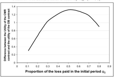
In Figure 2, we let the proportion of the loss paid in the initial period vary while keeping all other parameters constant. We see in both Panel A (where the discount factor is high) and Panel B (where the discount factor is low) that for a single event, the relationship between DU and α0 is that of an inverted
parabola. This illustrates Proposition 5. For high values ofδas in Panel A, we see that the agent is always better of with a CMR contract than an OB contract, no matter what the loss development pattern is. Proposition 5 says thatDU is increasing inα0 forα0<(1−δ)/(2−δ) = 0,09, and decreasing forα0 close
to one. This holds true in this Panel A.
For low values ofδas in Panel B, however,DU is negative for low values ofα0, but still increasing inα0
forα0<(1−δ)/(2−δ) = 0,33. Hence, agents are better offpurchasing an OB contract when the proportion
of the loss that is paid in the initial period is low and the agent discounts the future a lot. Asα0increases,
DU eventually becomes positive, which means that the CMR contract becomes preferred to the OB contract, and eventually reaches a maximum positive value. The advantage the CMR contract over the OB contract then decreases, but remains positive untilα0= 1. In our computations for this simplified framework where
the development pattern is short, the value ofDU is positive for most combinations ofα0 andδ.
Figure 2. Expected utility of having a Claims-made contract compared to an Occurrence contract as the proportion of the loss that is paid in the initial period
(α0) varies, with an agent who lives for two periods (T = 2), when losses fully
develop over two periods (n= 1) and the discount rate is relatively high (δ= 0.9). Panel A. The discount factor is relatively high (δ= 0.9).
0 0.2 0.4 0.6 0.8 1 1.2 1.4 0 0.1 0.2 0.3 0.4 0.5 0.6 0.7 0.8 0.9
Proportion of the loss paid in the initial period
D iffe re n ce b etw ee n th e U ti lit y o f th e C M R co nt ra ct a n d th e ut ilit y of t h e O B c o nt ra ct α0
Panel B. The discount factor is relatively low (δ= 0.5).
-0.4 -0.2 0 0.2 0.4 0.6 0.8 0.000 0.200 0.400 0.600 0.800 1.000
Proportion of the loss paid in the initial period
D if fe re n ce be tw ee n t h e U tilit y of t h e C M R co nt ra ct a n d t h e ut ilit y of t h e O B c o nt ra ct α0
Finally, we find that the CMR advantage decreases when the number of possible events, T, increases. With more than one potential event, that is whenT >0and the agent insures for all his professional life, the
increasing weight of the discounted OB premium plays for the OB contract andDU is more often negative.
6
Conclusion
The goal of this paper was to compare the relative efficiency of two types of insurance contracts that seek to offer policyholders financial protection against lawsuits brought upon them while exercising their professional activities. These two types of contracts are known as the traditional and well-knownoccurrence based insurance contract, whereby insured agents are covered for losses that their incur in the policy year no matter when the claim isfiled in the future, and theclaims-made and reported insurance contract, whereby insured agents are covered for losses that are reported during the policy year no matter when the losses was incurred in the past. Claims-made contracts are popular in liability lines and account for 75% of the total earned premiums in the medical malpractice liability insurance line of business. At the same time, claims-made contracts are mostly inexistent in property insurance lines. Claims-made contract are also the default type of contract in the case of directors’ and officers’ liability insurance and many other professional liability insurance coverages. And although claims-made contracts also exist to cover product liability losses, they are much less popular than the traditional occurrence based contract since only 15% of product liability insurance contracts are claims-made.
The model we developed in this paper was seeking to explain the coexistence of the two types of contract and to answer the following two empirical questions:
• Why are claims-made contract more popular in long-tail lines than in short-tail lines? And
• Why are claims-made contract more popular in personal liability lines than in commercial liability lines?
The theory proposed by Doherty (1991) suggests that claims-made contract are an answer to an increase in the uncertainty of the legal environment in which insurers operate. This theory explains well why claims-made contracts should be more prevalent in long-tail lines, but it does not explain why claims-claims-made contracts should not be more prevalent in personal liability lines. In fact, risk averse individuals should be more reluctant to assume the legal environment uncertainty than risk neutralfirms. In contrast, the theory we propose based on the loss development pattern of liability claims and the difference between the discount factors of insured agents and insurance companies is able to explain the two stylized facts of short-tail versus long-tail lines and of personal versus commercial insured agent.
Another possible explanation for the prevalence of CMR over OB contracts in certain economic context, but one we did not examine in the current paper, is the uncertainty, at the time the claim isfiled, as to when the loss was incurred exactly in the past. When it is hard to pinpoint the exact time a loss was incurred it becomes difficult to identify which past insurer is responsible for the claim that isfiled today. It may then be optimal in terms of transaction costs to have a CMR policy rather than an OB policy. With a CMR policy, there is no uncertainty as who isfinancially responsible for the claim since it is the insurer underwriting the contract at the time the claim isfiled. If on the other hand it is easy to pinpoint the insurer who isfinancially responsible, then it is less obvious that a CMR contract would be preferred. Finally, if there are solvency issues with past insurers, an insured agent could prefer to purchase a series of CMR contracts over his lifetime rather than face the possibility that, in the future, the insurer who underwrote the contract becomes bankrupt and unable to cover the loss. Using a simple Markov-switching approach with bankruptcy being an absorbing state, it is clear that the longer a loss takes to fully develop, the more likely the insurer will be bankrupt and unable to pay when the claim isfinallyfiled. One other theory developed by Posner (1986) suggests that insurers switching to claims-made contracts were willing to continue underwriting the risk of patient injuries but did not want to assume the timing risk (i.e., when the compensation is be paid) and the corresponding inflation and investment risks. This Posner approach is somewhat linked to our approach in the sense that the switch to claims-made could be explained by a reduction in the insurers’ discount factor
δI.
The theoretical approach we used in this paper to address why and when insured agents should prefer a claim-made and reported insurance contract to an occurrence-base insurance contract allows us to draw three main conclusions. First, if agents seeking insurance are risk neutral (and therefore purchase insurance only because, for instance, they are mandated to do so by the legislation), then, only the differences in the discount rate of the insurer and of the agent will determine the purchase of such or such contract. Second, if there is some level of uncertainty as to what future losses will be, then a CMR contract can indeed help insurers get rid of some level of uncertainty as in Doherty (1991). Because a CMR insurance contract allows to price insurance using all the information that is available at the current time, neither the agent nor the insurer are locked in a contract that was signed in a past period under conditions that may no longer apply. Finally, if agents are risk averse, they may prefer the claims-made insurance contract to defer payments the first periods of their professional lives to future periods so that their income is a bit smoother than under an occurrence insurance contract.
7
References
1. Berger, Lawrence A., J. David Cummins, and Sharon Tennyson (1992). Reinsurance and the Liability Insurance Crisis. Journal of Risk and Uncertainty 5(3), 253-272.
2. Born, Patricia and M. Martin Boyer (2008). Claims-Made and Reported Policies and Insurer Prof-itability in Medical Malpractice. CIRANO working paper 2008s-13.
3. Cummins, J. David and Sharon Tennyson (1992). Controlling Automobile Insurance Costs. Journal of Economic Perspective 6(2), 95-115.
4. Doherty, Neil A. (1991). The Design of Insurance Contracts When Liability Rules Are Unstable.
Journal of Risk and Insurance 58(2), 227-246.
5. Doherty, Neil A. and Georges Dionne (1993). Insurance with Undiversifiable Risk: Contract Structure and Organizational Form of Insurance Firms,Journal of Risk and Uncertainty, 6: 187-203.
6. Harrington, Scott E., Patricia M. Danzon, and Andrew J. Epstein (2008). ‘Crises’ in Medical Malprac-tice Insurance: Evidence of Excessive Price-Cutting in the Preceding Soft Market,Journal of Banking and Finance, 32: 157-169.
7. Nye, Blaine F. and Alfred E. Hofflander (1987). Economics of Oligopoly : Medical Malpractice Insur-ance as a Classic Illustration. Journal of Risk and Insurance54(3), 502-519.
8. Nye, Blaine F. and Alfred E. Hofflander (1988). Experience Rating in Medical Professional Liability Insurance. Journal of Risk and Insurance 55(1), 150-157.
9. Posner, James R. (1986). Trends in Medical Malpractice Insurance: 1970-1985,Law and Contemporary Problems, 49 (2): 37-56.
10. Sloan, Frank A., Randall R. Bovbjerg, and Penny B. Githens (1991). Insuring Medical Malpractice. New York: Oxford University Press.
8
Appendix: Proofs
Proof of Proposition 1. Because agents are risk neutral, they will purchase the contract whose cost is smaller. In other words, the CMR contract will be preferred to the OB contract if and only ifΠb <Π. We have
Π= T X t=0 δtAP = T X t=0 δtA n X i=0 δiIαiL= Ã T X t=0 δtAL ! Ã n X i=0 δiIαi ! ,
andΠb can be simplified into
b Π = n X t=0 δtA t X i=0 αiL+ T X t=n+1 δtA n X i=0 αiL+ TX+n t=T+1 δtA n X i=t−T αiL (1) = n X i=0 αi ÃT+i X t=i δtA ! L= n X i=0 αiδiA Ã T X t=0 δtA ! L (2) = Ã T X t=0 δtAL ! Ã n X i=0 δiAαi ! (3)
Hence,Πb <Πif and only ifδA< δI. QED¤.
Proof of Proposition 2. With a potential event in each of thefirstT periods of the agent’s life, the sequence of OB premiums is Pt= n X i=0 αiδiIE(Lt+i),
that is, each periodtOB premium depends on thenfuture expected losses. The CMR premiums take only current losses into account. However, these losses evolve with time.
b Pt= ⎧ ⎪ ⎨ ⎪ ⎩ Pt i=0αiE(Lt) ift < n Pn i=0αiE(Lt) ifn≤t≤T Pn i=t−TαiE(Lt) ifT+ 1≤t≤T+n. (4)
A risk neutral agent will choose the contract that offers the lowest expected discounted sum of premiums. We have P = T X t=0 δtAPt= T X t=0 δtA Ã n X i=0 αiδiIE(Lt+i) ! = n X i=1 αi T X t=0 δtAδiIE(Lt+i) (5) and b P = n X t=0 δtA Ã t X i=0 αiE(Lt) ! + T X t=n+1 δtA Ã n X i=0 αiE(Lt) ! + TX+n t=T+1 δtA Ã n X i=t−T αiE(Lt) ! = n X i=0 αi T X t=0 δtA+iE(Lt+i) (6)
Then,P >Pbif and only if δI > δA. QED¤
Proof of Proposition 3. Suppose a potential event in period 0 with an invariant loss distributionLdeveloping overn+ 1periods and such thatE(L) =Lregardless of the period the claim is made. Suppose there are no potential event after period 0.
With the same discount factor δA=δI =δ∈[0,1], the agent’s intertemporal utility over periods0ton
isUOB(δ)in a OB contracts andUCM R(δ)in a CMR contract, such that
DU(δ) =u(Y −α0L)−u(Y − n X i=0 αiδiL) + n X i=1 δi¡u(Y −αiL)−u(Y)¢
It is easy to verify that DU(0) = 0 since UCM R(0) = u(Y −α0L) = UOB(0). We then show that
DU(1)>0. UOB(1) = u(Y −L) +nu(Y) UCM R(1) = n X i=0 u(Y −αiL)
sincePni=0αi= 1. By concavity ofu, we have that
αju(Y −L) + n X i=0,i6=j αiu(Y)< u(αj(Y −L) + n X i=0,i6=j αiY) =u(Y −αjL), so that n X j=0 ⎛ ⎝αju(Y −L) + n X i=0,i6=j αiu(Y) ⎞ ⎠< n X j=0 u(Y −αjL), and then, u(Y −L) +nu(Y)< n X j=0 u(Y −αjL). Hence,DU(1)>0. QED¤. Proof of Proposition 4.
Let us differentiateDU with respect toδ. We have
∂DU ∂δ = n X j=1 jαjδj−1Lu0(Y − n X i=0 αiδiL) + n X j=1 jδj−1¡u(Y −αjL)−u(Y) ¢ = n X j=1 jδj−1£αjLu0(Y − n X i=0 αiδiL)− ¡ u(Y)−u(Y −αjL) ¢¤
The concavity of u implies that αjLu0(Y −αjL) >[u(Y)−u(Y −αjL)] (linear approximation of the
difference is larger than the difference). Hence, ∂DU∂δ is positive atδ= 1. Forδin[0,1), the sign is ambiguous however.
Let us denoteˆδj the value ofδfor whichPni=0αiδˆj i
=αj. Then, forδ >δˆj we havePni=0αiδi> αj and
then, αjLu0(Y − n X i=0 αiδiL)> αjLu0(Y −αjL)> u(Y)−u(Y −αjL).
Let us denote δ∗ = maxn
j=0δˆj. We have, then, that αjLu0(Y −Pni=0αiδiL) > αjLu0(Y −αjL) >
u(Y)−u(Y −αjL)for allδ≥δ∗.Hence ∂DU∂δ(δ) >0forδ≥δ∗.
QED ¤.
Proof of Proposition 5. Let us see what happens toDU when we slightly alterα0.
∂DU ∂α0 = −Lhu0(Y −α0L)−δT+1u0(Y −(1−α0)L) i + " (1−δ)L T X t=0 δtu0(Y −(α0+ (1−α0)δ)L) # ∂DU ∂α0 × (−1/L) = hu0(Y −α0L)−δT+1u0(Y −(1−α0)L) i −(1−δT+1)u0(Y −(α0+ (1−α0)δ)L),
becausePTt=0δt= (1−δT+1)/(1−δ). That is, ∂DU∂α0 is positive if
[u0(Y−α0L)−u0(Y−(α0+ (1−α0)δ)L)]
−δT+1[u0(Y−(1−α0)L)−u0(Y−(α0+ (1−α0)δ)L)]≤0
The term in thefirst bracket is always negative becauseα0L≤(α0+ (1−α0)δ)Lforα0<1and u0 is
decreasing. The term in the second bracket is positive if1−α0≥α0+ (1−α0)δ. That is, ∂DU∂α0 is positive if
α0≤ 12−−δδ. Note that the fraction 21−−δδ is decreasing inδ, with maximum value 1/2 whenδ= 0and minimum
value 0 whenδ= 1.
For anyα0greater than 12−−δδ, the derivative ∂DU∂α0 can be positive or negative. Let usfind the limit value
of this derivative asα0→1. We have
∂DU ∂α0 |α0→1 = −Lhu0(Y −L)−δT+1u0(Y)i+ (1−δ)L T X t=0 δtu0(Y −L) = L " δT+1u0(Y)−u0(Y −L) Ã 1− T X t=0 δt+δ T X t=0 δt !# = δT+1[u0(Y)−u0(Y −L)]L <0