Essays on applied political economics

OpenBU http://open.bu.edu

Theses & Dissertations Boston University Theses & Dissertations

2016

Essays on applied political

economics

https://hdl.handle.net/2144/17717

GRADUATE SCHOOL OF ARTS AND SCIENCES

Dissertation

ESSAYS ON APPLIED POLITICAL ECONOMICS

by

MIRKO KLAUS FILLBRUNN Diplom, University of Duisburg-Essen, 2005

Submitted in partial fulllment of the requirements for the degree of

Doctor of Philosophy 2016

MIRKO KLAUS FILLBRUNN 2016

First Reader

Jawwad Noor, PhD

Associate Professor of Economics

Second Reader Dilip Mookherjee, PhD Professor of Economics Third Reader Daniele M. Paserman, PhD Professor of Economics

I greatly thank Jawwad Noor for all his time and support when writing my dissertation and completing my PhD. I am grateful to Dilip Mookherjee and Daniele Paserman for their advice and helpful discussions. Many people helped me nish my PhD and, in no particular order, I want to thank Levent Altinoglu, Laurent Bouton, Felipe Cordova, Juan Ortner, Carlos Ramos, Ben Solow, Patricio Toro, and Fan Zhuo. And of course, I thank my family, and in particular my mother Iris Fillbrunn.

MIRKO KLAUS FILLBRUNN

Boston University, Graduate School of Arts and Sciences, 2016 Major Professor: Jawwad Noor, Associate Professor of Economics

ABSTRACT

This dissertation consists of three essays on the determinants of voting behavior.

In Chapter 1, I empirically examine why candidates who are listed rst on voting ballots enjoy substantial advantages such as winning 10% more elections. I use Californian election data where ballot order is randomized but identical for every voter. With these data, I provide new empirical regularities on how such ballot order eects change with the number of votes available to voters and candidate popularity. I show that these patterns are dicult to reconcile with existing models in which ballot order directly aects a voter's choices. In Chapter 2, I propose a novel theory of ballot order eects where rational voters respond to behavioral voters and then amplify the advantage of candidates listed rst due to the inherent strategic complementarity in voting. My model is an extension of a standard vot-ing model and allows me to explicitly model the interaction of dierent types of voters. I estimate my model using a simulated method of moments and nd that the interaction be-tween voters is empirically important: rational order eects account for around half of total ballot order eects in terms of vote shares (votes gained just for being listed rst), while also reducing the number of behavioral voters necessary to explain the data in other dimensions as well. Motivated by these ndings, I suggest new policies to address ballot order eects. In Chapter 3, I investigate how newspaper consumption aects political engagement. To circumvent potential endogeneity issues, I use variation in European languages as an instru-ment for newspaper consumption. Specically, I consider variation in how much physical space languages require to express some given information content. I rst estimate such language eciency from large bilingual text compilations. Using a European-wide survey that spans 18 dierent languages, I nd that respondents who speak ecient languages are

to a large variety of alternative specications. Using language eciency as an instrument for newspaper consumption, I nd that newspaper consumption increases turnout and political interest of immigrants.

1 Empirical Patterns of Ballot Order Eects 1

1.1 Literature Review . . . 3

1.2 Empirical Patterns of ballot order eects . . . 4

1.2.1 Data . . . 4

1.2.2 Total ballot order eects . . . 6

1.2.3 Conditional ballot order eects . . . 7

1.2.4 Empirical patterns . . . 13

1.3 Alternative pure boundedly-rational models . . . 15

1.3.1 Tie-breaking model . . . 15

1.3.2 Satiscing . . . 19

1.3.3 Utility-bump model . . . 19

1.4 Conclusion . . . 22

1.5 Appendix . . . 22

1.5.1 Proofs: Purely behavioral models . . . 22

2 Strategic Voting and Ballot Order Eects 29 2.1 Introduction . . . 29

2.2 Literature review . . . 32

2.3 Model . . . 34

2.3.1 Environment . . . 34

2.3.2 Voting equilibrium . . . 37

2.3.3 Mechanisms in the model . . . 43

2.4 Empirical evaluation . . . 47 vii

2.4.2 Estimation of rational order eects - vote shares . . . 49

2.4.3 Counterfactual analysis - winning advantage . . . 53

2.4.4 Estimation of behavioral share - two-candidate elections . . . 55

2.4.5 Discussion of results . . . 57

2.5 Conclusion . . . 59

2.6 Appendix . . . 60

2.6.1 Denitions and assumptions . . . 60

2.6.2 Formal analysis of rational order eects . . . 62

3 Newspapers, Voting, and Languages 79 3.1 Introduction . . . 79 3.2 Language eciency . . . 83 3.2.1 Language eciency . . . 84 3.2.2 Estimation . . . 85 3.3 Theory . . . 90 3.3.1 Supply side . . . 90 3.3.2 Demand side . . . 95 3.3.3 Combined predictions . . . 97

3.4 Empirical analysis - Language eciency and newspapers . . . 98

3.4.1 Identication discussion . . . 98

3.4.2 Individual-level evidence . . . 100

3.4.3 Aggregate-level evidence . . . 106

3.5 Voter Turnout and Newspapers . . . 110

3.6 Appendix . . . 113

3.6.1 Proofs . . . 113

3.6.2 Tables . . . 116

Bibliography 118

1.1 Data, Order Eects by vote share percentile, 3-candidate election, one vote

per voter, one winner . . . 9

1.2 Data, order eects by vote share percentile, 3-candidate elections. . . 10

1.3 Data, order eects by vote share percentile, 4-candidate elections. . . 11

1.4 Data, Dierence of order eects between single-vote elections and multi-vote elections by percentile with 95% condence bounds, 3-candidate elections. . . 12

1.5 Pure Tie-breaking model prediction . . . 17

1.6 Satiscing model prediction, advantage of candidates listed rst over candi-dates listed second, and advantage of candicandi-dates listed second over candicandi-dates listed third. . . 20

1.7 Data, advantage of candidates listed rst over candidates listed second, and advantage of candidates listed second over candidates listed third. . . 21

2.1 Rational order eects as a function of whether a candidate is in the running . 44 2.2 Num. example of order eects in model, 3-candidate elections. . . 48

2.3 Proof proposition 9 illustration, no behavioral voters . . . 77

2.4 Proof proposition 9 illustration, with behavioral voters . . . 78

3.1 Sample sentences from 4 dierent versions of the JRC Acquis corpora . . . 86

3.2 New York Times 1914 front page . . . 91

Chapter 1 and Chapter 2

a0, a1, a2, a00, a01, a02 Coecients on how vote share varies by percentile ai. . . Action/votes of voter i

aij. . . Vote of voter i for candidate j

A. . . Set of all possible actions

b. . . ballot order eect

b(q). . . conditional ballot order eect at vote share percentile q

B(a, b) . . . Ballot order eects from vote share percentile a to vote share

per-centile b

BOE . . . Ballot Order Eects

ck. . . Candidate k in an election

Ckj. . . Control variables

CDF . . . Cumulative Distribution Function CEDA . . . California Elections Data Archive

CI . . . Condence interval

CSD . . . Community Services & Development D . . . Data set

E. . . Expectation

exp . . . Exponential function

Fkj . . . Indicator whether candidatek is listed rst in election j

F(ε;c). . . Mean-zero distribution ofεij

G(U). . . Distribution of candidate mean utilities across elections

1)

Hkj. . . Indicator whether candidate k in election j has a vote share associated

with a high vote share percentile

H1. . . Probability that a voter prefers candidate 1 over all other candidates Hk,m−1 . . . CDF of the k-th lowest utility of a voter when there are m-1

candi-dates

m . . . Number of candidates in an election

M . . . Some large number ¯

M . . . Threshold for a large number N. . . Number of voters in an election N(0,1). . . Standard normal distribution

opp(ck). . . Competing candidate of candidate ck

pi(ck, cj). . . Perceived pivot probability

p(ck|ai). . . Probability of candidate ck winning given action ai

p . . . p value P(·) . . . Probability of

q. . . vote share percentile

Qk. . . CDF of vote shares of ballot position k

¯

q. . . Vote share percentile threshold R2. . . Coecient of determination r. . . Expected vote share rank s. . . Random draw of voters

tk(s). . . Vote share of candidate k given random draw s

T . . . Sum of all votes given out divided by the number of voters multiplied by the number of votes per voter

uy_i . . . Utility of voter i giiven ballot order y

U(ai). . . Expected utility for behavioral voter i given actionai

˜

ui(ck|p). . . Expected utility voter i of voting for candidateck given pivot

prob-abilities

˜

ui(ai|p). . . Expected utility voter i of voting according to ai given pivot

proba-bilities

uR. . . Aspiration level of a voter u. . . A voter's utility for candidates uij. . . A voter i's utility for candidate j

Uj . . . Mean utility for candidate j across all voters in an election

v. . . Vote

vk. . . Vote for candidate k

w . . . Number of candidates that may win the election and number of votes a voter may cast, assumed identical

y. . . Ballot ordering

Y . . . Set of all possible ballot orderings c. . . Finite, positive random number

. . . Preferred to

β. . . Dierence between ballot order eects before and after threshold µ . . . Scale parameter of the logit distribution

βT . . . Coecient to be estimated in Tie-breaking model

η. . . Utility bump

Exp(ν). . . Exponential distribution with parameterν

τkj . . . Vote share of candidate in ballot position k in election j

¯

τk . . . Average vote share of candidates in ballot position k across all

elec-tions in the data P

. . . Summation

λ. . . Share of behavioral voters

εkj. . . Econometric error at the candidate-election level

β1 . . . Eect of triple interaction ofFkj,qkj, andgj on vote share

β2 . . . Eect of triple interaction ofFkj,qkj2 , andgj on vote share

θ . . . A voter's type

C . . . Set of candidates in an election

C_x . . . Set of candidates in an election that tie for the x-th place

ψk(σF) . . . Share of strategic voters preferring candidateck over competing

can-didate when the distribution F has standard deviation σF

R. . . Set of real numbers

εij. . . Idiosyncratic utility shock of voter i for candidate j

σF(c). . . Standard deviation ofF(ε;c)

∈. . . Element in

\. . . Without a set operator . . . Much larger

Chapter 3

a . . . Space occupied by advertisement in a newspaper

Bq. . . Demand parameter given quality q

c . . . Cost parameter

CIA . . . Central Intelligence Agency D . . . Demand

DE . . . German

DGT . . . European Commission's Directorate-General for Translation corpus EN . . . English

EU . . . European Union

Europarl . . . . Corpus made of EU parliament speeches

EU Bookshop Corpus made of phrases from the EU bookshop xiv

F(c) . . . Distribution of cost parameters FOC . . . First order condition

FR . . . French

GDP . . . Gross Domestic Product

i. . . Space occupied by images in a newspaper or respondent/individual i IT . . . Italian

JRC-Acquis . Aligned multilingual corpus of the Joint Research Centre of the Eu-ropean Commission

k . . . Some consumer k L . . . Language eciency

L. . . Set of readers who would read at language eciency L NoSchool . . . . Population with no schooling

ns . . . Number of repetitions

nwsatall . . . Whether individuals said they read newspapers at all

nwsptot . . . How much time individuals spend reading newspapers on an average weekday

NYT . . . New York Times p . . . p value

P. . . Price

P∗. . . Optimal price

Pop1564 . . . Population between the ages of 15 and 64 PPP. . . Purchasing Power Parity

q. . . Quality ˜

q. . . Perceived quality ¯

Q. . . Average newspaper quality in the market

SETimes . . . . Corpus of news articles of the Southeast European Times t . . . Space occupied by text in a newspaper

¯

T. . . Average newspaper reading time

UN . . . United Nations

UNESCO. . . . United Nations Educational, Scientic and Cultural Organization Urban . . . Population living in an urban environment

YrsSchooling Average years of schooling

sigma. . . Standard error π. . . Prot

ε. . . Share of newspapers in a country that choose high quality εk. . . Mean-zero shock to quality perception

∂. . . Partial derivative βx

L. . . Eect of language eciency on statistic x

∈. . . Element of

δ. . . Some parameter

Empirical Patterns of Ballot Order Eects

There is evidence that the order in which alternatives are presented can aect how a person chooses from these alternatives: for example, Jacobs and Hillert [2014] argues that the alphabetical position of the rst letter of a company's name inuences its trading activity in stock markets; or Einav and Yariv [2006] nds that academic success is correlated with an economist's surname's initial; or the more anecdotal observation that many rms in the Yellow Pages have names that start with AA or AAA. It is also well known that order eects are an important feature of elections. A quote from a 1940 U.S. court case reads, It is a commonly known and accepted fact that in an election [...] those whose names appear at the head of the list have a distinct advantage.1_{Accordingly, 30 US states directly randomize}

the ordering of candidates on the voting ballot to minimize these (undesirable) ballot order eects (BOE) (Miller [2010]). There is also substantial empirical evidence of ballot order eects in the literature: for example, Ho and Imai [2008] nds ballot order eects substantial enough to have changed the outcome of 12% of the primary elections studied therein.

While there are some theoretical explanations of ballot order eects using behavioral models, the majority of the empirical literature has focused on establishing their existence (Ho and Imai [2008], Miller and Krosnick [1998]) instead of their underlying cause (Meredith and Salant [2013]). As such, the origin of order eects in elections is still a puzzle. In this chapter, I try to understand such ballot order eects better. To do this, I rst present new empirical regularities of ballot order eects. I nd that these patterns are inconsistent with the underlying intuition of the leading models in the literature.

More specically, I use a data set containing election outcomes of local Californian elections from 1995 to 2012. In my data, ballot positions are randomly assigned before the election, but the same for each voter. I rst construct the empirical cumulative distribution functions (CDFs) of vote shares for each ballot position across all elections in the data. I then compare the CDFs for candidates listed rst on the ballot to the average of the CDFs of candidates not listed rst. Without any order eects, these two CDFs should be identical due to the randomly determined ballot order. However, I nd that in three-candidate elections where voters may elect one candidate to win (single-vote elections), these two CDFs are not only dierent, but they follow a particular pattern:

• Pattern 1: in single-vote elections, the horizontal dierence between the two CDFs, i.e., the dierence in vote shares for a given percentile, is lowest for low and very high vote share percentiles, and largest for intermediate candidates.

I nd a similar pattern in four-candidate single-vote elections.

Why is this potentially interesting? Percentiles of vote shares are related to a candidate's popularity, thus pattern 1 may be interpreted such that unpopular and very popular can-didates benet the least from being listed rst, while intermediate cancan-didates benet most. This can provide some guidance when comparing dierent models of ballot order eects.

Next, I repeat the analysis for three-candidate elections where voters may elect all but one candidate in the election (multi-vote election), i.e., voters may vote for two candidates to elect two winning candidates, for instance voters may vote for two seats on the school board.

• Pattern 2: in multi-vote elections, the dierence in CDFs is relatively constant, i.e., similar for all percentiles.

Again, a similar pattern can be found in four-candidate elections with three votes per voter.2

Lastly, I discuss the consistency of other behavioral models of ballot order eects with the observed empirical patterns. While these do not directly make predictions based on a

2_{There are not enough elections to conduct the same analysis with ve candidates (59) compared to}

candidate's vote share percentile, ballot order eects may be correlated with a candidate's popularity, which itself can be related to a candidate's vote share percentile. As it turns out, various basic behavioral models where ballot order is used to complete a voter's prefer-ences are dicult to reconcile with the data. A model where voters gain extra utility when voting for candidates listed (Miller and Krosnick [1998]) rst generates hill-shaped ballot order eects (pattern 1) but does so for both single-vote elections and multi-vote elections, and is thus unable to generate the relative atness of ballot order eects in multi-vote elec-tions with respect to candidate quality (pattern 2). A search model as in (Meredith and Salant [2013], Simon [1955], Ho and Imai [2008]) typically implies patterns 1 and 2 for both candidates listed rst and second, which is unlike what we see in the data.

1.1 Literature Review

My study is connected to the literature that investigates the empirical extent of ballot order eects and the psychological motivation behind it. Parts of my data set stem from Meredith and Salant [2013] which provides evidence for the existence of ballot order eects in Californian local elections. This study tests the implications of a theory in which voters are unsure about their favorite candidate (Satiscing), a prominent theory to explain ballot order eects. It shows that a simple model of Satiscing cannot alone explain the empirical pattern based upon a test comparing the advantages of the second-listed candidate and the third-listed candidate. Related, Ho and Imai [2008] examines Californian state elections and nds that while ballot order eects are not signicant in general elections, they are inuential in primaries and large enough to have changed the election winner in around 12% of primary elections. Their study considers a cognitive model akin to the Satiscing model. Last, Miller and Krosnick [1998] studies elections in Ohio and nds ballot order eects of around 2.5% vote share percentages.

1.2 Empirical Patterns of ballot order eects

In this section, I present my data set and dene ballot order eects formally. I investigate whether there are any regularities of ballot order eects that help us identify their sources. 1.2.1 Data

I use data from the California Elections Data Archive (CEDA), a publicly available collection of local Californian elections outcomes. These elections determine county supervisors, city council members, etc., in California's 58 counties and more than 1,100 school and community college districts.

The CEDA data set that I use includes a total of 9,905 elections from the years 1995 to 2012. Elections are usually held in March or June and in November during even years, together with the accompanying state-wide elections, and in November during odd years. Elections vary in their number of candidatesmand possible winners and votes per voterw.

Voters can cast as many votes as there are winners in almost all elections in my data set so I restrict my analysis to these types of elections. All elections are non-partisan, meaning that candidates are not allowed to state their party aliation if they have any.

Important for us, the California Secretary of State oce randomizes the ordering of candidates on the ballot roughly 80 days before Election Day (but after candidates decided to enter): they randomly draw a new alphabet and then order candidates by their names on all ballots in an election. As an example, if a new alphabet would be drawn to be A C B instead of A B C, Charlie would be listed before Brown. This random determination ensures that ballot order is uncorrelated with any characteristic of the candidates.3

In the data, slightly more than half of the elections are school board elections (5,843), a third are city council elections (3,377), and the remaining elections (853) are for county or city oces such as mayor, CSD/CSA director, etc. From the raw data set, I excluded

3_{This is not true randomization, as a candidate named Smith will never be between two Adams, but this}

randomization failure would only then be important if candidates responded to it, which is unlikely due to the small chance of it changing the ordering.

elections for which I did not have the ordering of candidates (4,102),4 _{the election data}

were incomplete (46), the number of potential winners did not coincide with the number of votes per voter (228) or the number of votes per voter was equal or higher than the number of candidates (188). I also exclude runo elections as they provide potentially dierent incentives for voters (1,034)5_{(Bouton [2013], Bouton and Gratton [2015]) as well as elections}

that cross county borders (249).

My data on ballot ordering for the years 1995 to 2008 comes from Meredith and Salant [2013] where applicable and I collect additional alphabets for the years 2008-2012.6 _{I assign}

ballot ordering manually according to these publicized alphabets, and Meredith and Salant [2013] shows that assigning ballot order manually matches the actual ballot order 97% of the time for the San Bernardino County, where discrepancies stem from confusion about what constitutes the last name of the candidate.

Every ballot contains multiple electoral races. I argue that this reduces the inuence of any single election on whether voters turn out, which I use as justication to assume exoge-nous turnout in my theoretical model later on. However, salient elections might inuence a voter's turnout decision, so I drop mayoral races as they may drive voters to the polls. Any remaining dierences in turnout are then captured by time or county xed eects.7

I run my baseline regressions excluding the 5% of elections with the lowest total number of votes cast (668), i.e., elections with less than 667 total votes. This restriction is motivated by the theoretical model of strategic voting that I use, which I discuss in more details below. In a nut shell, if elections are suciently large and the chance of a decisive vote diminishes, the choice of strategic voters can be characterized by relative preferences rather than utilities. Robustness checks suggest that alternative restrictions provide qualitatively similar results.

4_{The numbers refer to the amount of elections dropped after the previous step was executed.}

5_{My data set does not explicitly denote which elections are runo elections but rather indicates in rst}

round elections whether a candidate proceeded to the second round or potentially could have had. This allows me to easily distinguish rst rounds of runo elections from plurality elections. The second round of runo elections can then be inferred by comparing the set of candidates in two-candidate elections to elections of the previous election cycle.

6_{My assignment coincides for all but one election with Meredith and Salant [2013] for the overlapping}

year 2008.

7_{I use month and year dummies in most estimations but do not use their interactions. However, including}

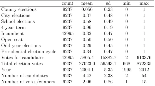
Below I present a few summary statistics in table 1.1. Half of all elections are open seat elections, i.e., without an incumbent running for oce, and roughly every third candidate is an incumbent, while elections have on average 27,023 votes (median 10,082 votes). Table 1.2 displays the number of elections in my data set for the types of elections I use most frequently.

count

mean

sd

min

max

County elections

9237

0.056

0.23

0

1

City elections

9237

0.37

0.48

0

1

School elections

9237

0.58

0.49

0

1

4 year term

9237

0.96

0.19

0

1

Incumbent

42995

0.32

0.47

0

1

Open seat

9237

0.50

0.50

0

1

Odd year elections

9237

0.29

0.45

0

1

Presidential election cycle

9237

0.34

0.47

0

1

Votes for candidates

42995

5805.4

15882.7

2

613376

Total election votes

9237

27023.0 56593.1

668

872335

Year

9237

2004.1

5.35

1995

2012

Number of candidates

9237

4.42

2.38

2

54

Number of votes/winners

9237

2.06

0.86

1

15

Table 1.1: Summary statistics # of votes per voter/winners # of candidates # of elections

1 2 1,988

1 3 546

1 4 143

2 3 1,179

3 4 804

Table 1.2: Number of elections by election type (after excluding small elections)

1.2.2 Total ballot order eects

I now dene Ballot Order Eects (BOE) formally. Suppose my data contains |D|elections where each ballot position kis associated with a vote share τkj in election j. Letτ¯k be the

average vote share of ballot position kacross all |D|elections in the data ¯ τk = 1 |D| |D| X j=1 τkj.

Without any ballot order eects and randomly determined ballot order, all ballot positions should on average have the same vote share when the number of elections|D|grows large. This follows directly from the law of large numbers and the independence of ballot order from any candidate characteristic. Thus, dene (unconditional or total) order eects as the dierence between the rst position's average vote share and that of the other ballot positions b= ¯τ1− 1 m−1 m X k=2 ¯ τk.

We could dene order eects for any other ballot position as well, but the data suggest that only the rst-listed candidate has consistently an advantage.

Table 1.3 provides a rst look at some statistics of the data. I regress whether a candidate won the election on an indicator of whether a candidate is listed rst (and dummies for election types(m, w)). The rst candidate on the list wins 7.43% more elections than other

ballot positions, which is a 12.3% increase in winning chances (1). I also run a similar regression using vote shares as outcome. On average, the rst-listed candidate has a 3.2% higher vote share than other ballot positions (2). These results are similar to previous estimates of unconditional order eects (Miller and Krosnick [1998]). In contrast, the second or third candidate on the ballot does not gain from the ballot ordering in elections with three or four candidates. In what follows, I will focus on ballot order eects regarding the rst-listed candidate only.

1.2.3 Conditional ballot order eects

Next, I want to explore how ballot order eects change with the popularity of the rst candidate and with how many seats a voter can vote for, xing the number of candidates in the election. I will do this by computing a ballot position's CDF over all elections in

(1)

(2)

(3)

(4)

VARIABLES

Winner Vote share Vote share Vote share

First

7.43***

3.25***

2.49***

2.93***

(0.699)

(0.222)

(0.666)

(0.559)

Second

-0.0757

0.773

(0.648)

(0.568)

Third

0.836

(0.540)

Election type dummies

Yes

Yes

Yes

Yes

# of candidates

any

any

3

4

Observations

40,843

40,843

5,175

7,572

R-squared

0.097

0.506

0.492

0.523

Robust standard errors in parentheses

*** p

<

0.01, ** p

<

0.05, * p

<

0.1

the data.8 _{This measure will not only relate to popularity but also allow me to compare}

popularity across dierent election types, which is not possible when directly using vote shares.9

For instance, the solid line in gure 1.1 is the CDF Q1 of the rst ballot position.

Similarly, we can also construct the average of the CDFs of all other positions, Qk, k > 1

, which is the dashed line in that gure. Without any ballot order eects, the two CDFs should be identical. However, I nd they are not the same. In order to measure this variation not captured by unconditional ballot order eects, dene a new measure called conditional ballot order eect. This is dened as the horizontal dierence between the CDF of the rst candidate and the average CDF of all the other candidates.

Formally, dene for any vote share percentile q the vote share of ballot position k at

8_{Meredith and Salant [2013] also consider how order eects with vote share percentiles, meanwhile for}

dierent reasons.

9_{The relationship between vote shares and popularity might dier across elections - a vote share of 50%}

Figure 1.1: Data, Order Eects by vote share percentile, 3-candidate election, one vote per voter, one winner

percentileq to beτk(q)so that

q =Qk(τk(q)).

Then, the denition of ballot order eects b(q) conditional on percentile q is

b(q) =τ1(q)− 1 m−1 m X k=2 τk(q).

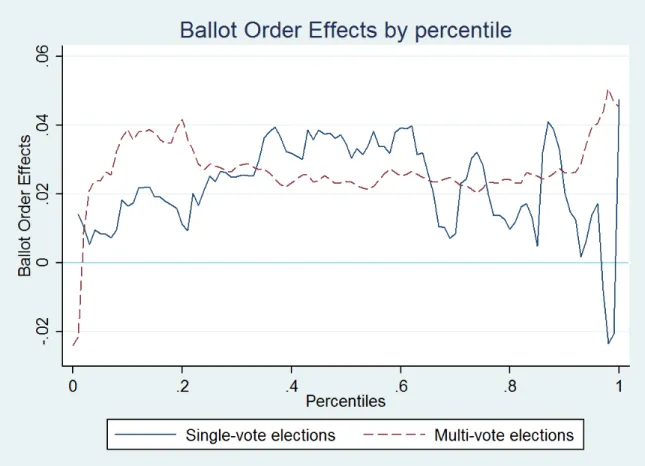
Conditional order eects b(q) are mapped in gure 1.2 for three-candidate elections with

percentiles on the x-axis for single-vote elections (solid line) and multi-vote elections (dashed line). Figure 1.3 provides the same graph for four-candidate elections. Without ballot order eects it must hold that|D| → ∞ ⇒τ¯k(q) = ¯τk0(q) for allk, k0.

Figure 1.4: Data, Dierence of order eects between single-vote elections and multi-vote elections by percentile with 95% condence bounds, 3-candidate elections.

1.2.4 Empirical patterns

I rst look at the empirical shape ofb(q)separately for three-candidate single-vote elections

and multi-vote elections as in gure 1.2. Ballot order eects in single-vote elections seem to have a large bump that starts around the 50th percentile and that extends to high percentile levels, while ballot order eects for the remaining percentile values seem more constant. In contrast, ballot order eects in multi-vote elections seem more level at around 2% for all percentiles. The endpoints of both graphs are more volatile as vote shares in extreme percentiles are more spread out so dierences between vote shares at these percentiles are more volatile with nite data.

Using a non-parametric estimation, I nd that conditional order eects in three-candidate single-vote elections are signicantly higher than in three-candidate multi-vote elections for percentiles 64% to 81%, as can be seen in gure 1.4.10

The pattern also seems to exhibit an inverted U-shape for high vote share percentiles, starting to increase around the 50% percentile and decreasing in the 70% percentiles.

To investigate this inverted U-shape formally, I regress vote share τkj on an interaction

of

• an indicator of whether a candidate kis listed rst Fkj in election j,

• a candidate's percentile qkj or squared percentileq_kj2 , and

• a group indicatorgj (single-vote vs. multi-vote elections),

which then comes out to the following regression equation, where I omit the coecients on the lower-order interaction terms and controls Ckj,

τkj = Ckj +Fkj +qkj+qkj2 +gj

10_{These regressions use vote shares as observed in the data. In an alternative regression, I rerun this}

analysis but partialling out the eects of incumbency from vote shares. The ndings are similar. When including more controls such as time and county dummies, the results become less powerful. I provide tables in the appendix.

+ Fkj·qkj+Fkj·q2kj+Fkj·gj+gj·qkj+gjqkj2

+ β1Fkj·qkj·gj +β2Fkj·qkj2 ·gj+εkj.

Control variablesCkj include dummies for election types, incumbency interacted with

elec-tion type, whether the elecelec-tion is an open seat elecelec-tion (i.e., no incumbent) and year, month, and county dummies.11 _{I estimate condence intervals using the t-percentile bootstrap}

method with 2,000 repetitions.

Table 1.4 presents the results. Specication (1) through (3) run the above regression for elections with three candidates, (4) and (5) for four-candidate elections. The point estimates of β1 and β2 suggest a hill shape in all specications.12 As can be seen from gure 1.2, the

dierence in three-candidate elections is signicantly hill-shaped for higher percentiles - the estimates of β1 and β2 imply a downturn at around the 75-th percentile (3).13 I conduct

additional robustness tests related to the composition of elections across election types, they generally conrm the ndings here.

(1) (2) (3) (4) (5)

VARIABLES % Vote Share Vote Share Vote Share Vote Share Vote Share

β1 Linear term 11.37* 10.88** 16.19*** 15.33** 17.85**

β2 Quadratic term -8.29 -7.50 -18.78*** -15.39** -17.78**

β1 >0&β2 <0 Yes Yes Yes*** Yes Yes*

# of candidates 3 3 3 4 4

Excluded percentiles 1% <50% 1%

Observations 5,139 5,037 2,571 3,804 3,724

R-squared 0.984 0.990 0.992 0.979 0.987

Bootstrapped t-percentile 2,000 repetitions, clustered by election *** p<0.01, ** p<0.05, * p<0.1

Table 1.4: Empirical patterns of ballot order eects.

11_{For this regression, I drop elections that are held in May as there are only very few of these in my data}

set.

12_{To test whether the estimated eects are due to the construction of percentiles, I manually assign a}

random ballot ordering (dierent from the one in the data) and rerun the regressions. However, these estimates yield insignicant results, supporting the validity of the results presented here.

13_{This regression uses only for upper half of percentiles. The quadratic function usingβ}

1 andβ2 has a

1.3 Alternative pure boundedly-rational models

So far I presented various empirical regularities of ballot order eects. Now I investigate whether other, purely behavioral voting models are consistent with these empirical regu-larities as well. While one can cook up non-rational models compatible with the data, in this section I consider some plausible behavioral models and derive testable implications with uncontrived distributional assumptions. As it turns out, these basic behavioral models are dicult to reconcile with the data which supports the importance of strategic voting in creating ballot order eects.

I consider three dierent types of models which dier in the underlying cause of ballot order eects: Tie-breaking, Satiscing, and a Utility-bump model. In all these models I assume that the share of strategic voters is zero, 1−λ = 0. All voters are thus either

behavioral or sincere voters (who always vote according to their preferences). Alternatively, one could dene these models with a positive share of strategic voters who are not aware of the rst candidate's advantage. I provide a formal analysis of these models in the online appendix.

1.3.1 Tie-breaking model

There are two senses in which a vote might be a tie-breaker: in the exact sense of breaking indierences in preferences, and in an approximate sense where the agent breaks ties between alternatives whose utilities dierences are below a certain threshold. I use the term tie-breaking as referring to the former version, while the latter one is a special case of the Utility-bump model I consider below. A model where voters are subject to primacy eects Miller and Krosnick [1998] is similar to the Utility-bump model.

In a Tie-breaking model, voters have preferences that are order-independent and they vote strictly according to these preferences (sincere voters), but they use the ballot order to break indierences in their preferences. Therefore, in this model I assume that two-way ties happen with positive probability to create order eects.14

Formally, a tie-breaking behavioral voter with order-independent utilityui= (ui1, ..., uim)

then chooses an action ai ∈ {0,1}m =A to maximizeU(ai)

U(ai) =

X

aik=1

uy_ik,

where for any candidate in ballot position j,ui1 =uik implies thatuyi1 > u y ik.

Let me provide some intuition for how ballot order eects in this model look like. First note that candidates only benet from being listed rst if they get a vote when rst on the ballot and no vote otherwise. In single-vote elections, this means candidates benet only if they tie for being the most-preferred candidate of a voter because in that case they get a vote after the tie is broken in their favor and otherwise only with a 50% chance. Similarly, in two-vote elections, candidates listed rst need to tie for being the second-most-preferred candidate of a voter to benet from their ballot position. But candidates who tie more often for being the second-most preferred candidate have, on average, a lower mean utility than those candidates that tie for most-preferred candidate. This means that ballot order eects in single-vote elections are largest for candidates that perform well and in multi-vote elections for candidates that perform badly. I show a numerical example of this pattern in gure 1.5.

To test the Tie-breaking model, I regress vote sharesτkj on interactions of

• an indicator of whether a candidate kis listed rst Fkj in election j,

• a group indicatorgj (single-vote vs. multi-vote elections),

• whether candidate'sk percentile is in the region with large ballot order eects Hkj =

       qkj >0.5 if gj = 1 qkj <0.5 if gj = 0

which then leads to the following regression

τkj =α+β

m−w

The Tie-breaking model predicts β≤0.

Note that we need to adjust the share of behavioral voters by m−w

m−1: in this model,

behavioral voters vote for the rst candidate, but also give w−1

m−1 votes to other candidates.

This translates to a bonus for the rst candidate of, on average, 1− _mw−₋1₁ = m_m−₋w₁ from

behavioral voters.

Below in table 1.5, I present the results for three-candidate elections. I nd that the estimate of β is positive and signicant, even when excluding the 1% extreme percentiles.

This suggests that a tie-breaking model is dicult to reconcile with the data as ballot order eects are not large enough for low-performing candidates in multi-vote elections.

(1)

(2)

VARIABLES %

Vote Share Vote Share

Large BOE

-22.05***

-21.18***

(0.429)

(0.388)

Share of behavioral voters

4.18***

4.27***

(0.786)

(0.713)

Single-vote election

-55.41***

-55.09***

(0.446)

(0.431)

Share of behavioral voters

×

large BOE

-0.203

-0.370

(1.088)

(1.046)

Share of behavioral voters

×

single-vote election

-2.269**

-2.329***

(0.941)

(0.874)

Single-vote election

×

large BOE

46.93***

45.42***

(0.707)

(0.654)

β

Single-vote election

×

First

×

large BOE

2.750**

2.986**

(1.378)

(1.337)

Percentiles

∈

[1%

,

99%]

Observations

5,175

5,073

R-squared

0.838

0.855

Clustered (by election) standard errors in parentheses

*** p

<

0.01, ** p

<

0.05, * p

<

0.1

1.3.2 Satiscing

A common theory used to explain ballot order eects is called Satiscing (Simon [1955], Meredith and Salant [2013], Miller and Krosnick [1998]). Here, voters do not gain extra utility when voting for the candidate listed rst. Instead, voters have some xed aspiration level when reading the ballot and they start reading it from the top. They vote for the rst candidates to satisfy this aspiration level and, if no candidate satises their aspiration level, they vote for their most-preferred candidates. This mechanism then produces an advantage for candidates listed early as they are more likely to be considered for a vote.

Due to the way we construct vote share percentiles, it is not directly possible to test the Satiscing model using the empirical regularities presented before.However, the Satiscing model implies that not only candidates listed rst enjoy an advantage, but also candidates listed second. A simulation of how ballot order eets look like in the Satiscing model can be seen in gure 1.6. In these three-candidate elections, the solid blue line represents the advantage of candidates listed rst over those listed second, and the black dashed line represents the dierence between candidates listed second and those listed third. In contrast, gure 1.7 shows the same statistics in the data. The dierence between being listed second and third is smaller in the data than the respective dierence in the simulated Satiscing model.This suggests that a Satiscing model cannot explain the empirical patterns we nd in the data.15

1.3.3 Utility-bump model

Lastly, I consider a Utility-bump model. Here, behavioral voters vote according to their order-independent preferences and, importantly, enjoy some utility bump favoring the rst-listed candidate. This model is similar to the Tie-breaking model introduced above, where rst-listed candidates receive an innitesimal utility bump sucient to break ties. Thus, ballot order eects are of similar shape.

15_{In fact, the empirical test for the Satiscing model is similar to Meredith and Salant [2013], who also}

Figure 1.6: Satiscing model prediction, advantage of candidates listed rst over candidates listed second, and advantage of candidates listed second over candidates listed third.

Figure 1.7: Data, advantage of candidates listed rst over candidates listed second, and advantage of candidates listed second over candidates listed third.

Let η > 0 be the utility bump for the rst-listed candidate. Voters choose an action ai∈ {0,1}m=Ato maximize U(ai)

U(ai) =

X

aik=1

uy_ik,

whereuy_i(c) =ui(c) +η if y(c) = 1and uyi(c) =ui(c)otherwise. I allow η >0 to be of any

size.

With a general utility bump that depends on a candidate's or an election's characteristics one could reproduce almost any shape of ballot order eects in the data. Thus, I need to put further restrictions on the model: rst, let the utility bump η be constant. Next,

I choose a particular distribution for the distribution of mean utilities G(U), namely an

exponential distribution Exp(ν). The exponential distribution allows me to analytically

derive the model's testable implications due to its convenient properties regarding order statistics (for example, the minimum of two exponentials is exponential as well).

This testable implication is similar to the one in the tie-breaking model. Therefore, as seen in table 1.5, the data reject this testable implication. This suggests that a utility bump model under these assumptions cannot explain the data because it fails to explain the relative atness of order eects in multi-vote elections.

1.4 Conclusion

In this chapter, I establish new empirical regularities of ballot order eects using local election data from California. I nd that ballot order eects change with the number of votes a voter may give out and the number of candidates in the election. I further discuss the consistency of other behavioral models of ballot order eects with the observed empirical patterns. While these do not directly make predictions based on a candidate's vote share percentile, ballot order eects may be correlated with a candidate's popularity, which itself can be related to a candidate's vote share percentile. As it turns out, various basic behavioral models where ballot order is used to complete a voter's preferences are dicult to reconcile with the data.

1.5 Appendix

1.5.1 Proofs: Purely behavioral models 1.5.1.1 Tie-breaking model:

Recall the following assumptions:

Three-way or higher-order ties in preferences have zero probability (but two-way ties have positive probability).

Assumption 2 F and G are symmetric around their medians and independent of election type. Median of F is 0 by denition ofF as it is symmetric and mean zero.

Proposition If two-way ties happen with positive probability and under as-sumptions 2 and 3, the dierence in ballot order eects for candidates with high and low percentiles in single-vote elections is the same as the reverse in multi-vote elections in the tie-breaking model, i.e.:

B(0,1 2;q, m,1)−B( 1 2,1;q, m,1) =B( 1 2,1;q, m, m−1)−B(0, 1 2;q, m, m−1).

To prove this, I show that ballot order eects in single-vote elections are simply the mir-rored ballot order eects of multi-vote elections. I.e., a candidate with some mean utility

U in single-vote elections gets ballot order eects x and a candidate with mean utility U0 =U + 2·(d−U) in multi-vote elections, where d is the median of the mean utility

distribution, also gets ballot order eects of size x. This then directly implies the result.

Proof. Since candidate entry into the election is independent (assumption A), we can treat an election withmcandidates as an election withm−1candidates with anm-th candidate

entering. I now introduce some notation relating to order statistics: deneFk,m−1to be the

distribution of the k-th order statistic of m−1 independent random variables distributed

according to F. I.e., the distribution of the k-th lowest value of a m−1×1 vector, where

each entry is drawn independently according toF. Similarly, iff is the pdf ofF, letfk,m−1

be the pdf of the k-th order statistic of m−1 independent random variables.

Then, let Hk,m−1 be the CDF of the k−th lowest utility ui of a voter. By denition,

this is a combination of the mean utility distribution Gand the idiosyncratic utility shock

distributionF. Now consider a xed mean utilityU of a candidate. Due to the assumption

of independent errors (assumptions B and C), ballot order eectsb(U) for a candidate with

mean utilityU in an election with mcandidates andw votes per voter andk=m−w can

be written as the probability that voter'siutility for them-th candidate is the same as that

of the candidate with the k-th lowest utility for voteri:

b(U, k) = λ

Z b

a

where the rst part denotes the probability that thek−last candidate gets a utility of ui

for voter i and the second term that the candidate with mean utility U gets a utility of ui for voter i, i.e., that they tie. Remember that three-way or higher-order ties have zero

probability.

Letdbe the median ofH. The properties of order statistics imply with the assumption

of symmetry of both F andG thathk,m−1(x) =hm−k,m−1(x+ 2·(d−x)), as it holds that hk,m−1(x)

hm−k,m−1(x)

= 1−H(x) H(x)

and hk,m−1 and hm−k,m−1 have the same support [a,b]. Therefore, for any U, dene

U0=U+ 2·(d−U).

Note that dis also the median of Gas the distribution of F has zero mean and, due to its

symmetry, also a median of zero. We then have that

b(U0, m−k) = λ Z b a hm−k,m−1(ui)·f(ui−U0)dui = λ Z b a hk,m−1(ui+ 2·(d−ui))·f(−ui+U0)dui = λ Z b a hk,m−1(ui+ 2·(d−ui))·f(−ui+ 2·d−U)dui = λ Z b a hk,m−1(−ui+ 2·d)·f(−u+ 2·d−U)dui = λ Z −a+2d −b+2d hk,m−1(vi)·f(vi−U)dvi

where vi = −ui+ 2d. Since we assume that G and f are symmetric and independent, it

follows that H is symmetric. Thus, a+b= 2d, so that then

b(U0, m−k) = λ

Z −a+2d −b+2d

= λ

Z b

a

hk,m−1(vi)·f(vi−U)dvi

= b(U, k).

Note that percentiles and mean utilites are one-to-one related in this behavioral model because, rstly, behavioral voters are sincere and, secondly, ballot order eects are due to indierences in preferences - a candidate with higher mean utility would simply have a higher utility and thus not need to rely on ballot ordering. Now dene the sum of ballot order eects over percentilesx to x¯ in an election withw votes as, givenm,

B(x,x¯;w= 1) = m−1 m−w

Z x¯

x

b(Uj)dG(Uj(q)).

The result follows from integrating over the support of G.

1.5.1.2 Utility-bump model

Assumption 4: The utility bump η is constant across elections and identical

across all voters.

Proposition Under assumptions 1, 3, 4, and if the distribution of mean utility

G is exponential with parameter ν > 0, it then holds for any η, ν > 0 in the

utility-bump model that in three-candidate elections for suciently lowσF:

1 2B(0.5,1;w= 1)− 1 2B(0,1;w= 1)−[ 2 3B(0, 1 2;w= 2)− 1 3B( 1 2,1;w= 2)]<0.

The proof is similar to the one for a tie-breaking model. However, due to the more compli-cated nature of an unrestricted utility bump, I need to rely on parametric assumptions for mean utility distributions.

Proof. With the assumption about behavioral voters' utilities that σF → 0, the composite

entry into the election is independent, consider an election withm−1candidates into which

them-th candidate enters.

Consider a utility bump model where candidates listed rst enjoy a utility bump η. A

candidate gains from behavioral voting if the behavioral voter values the candidate below thew-th candidate without the utility bump, and above thew-th candidate with the utility

bump, where wis the number of votes per voter. To capture the ranking of utilities, dene Fk,m−1 to be the distribution of the k-th order statistic of m −1 independent random

variables distributed according to F - i.e., the distribution of the k-th lowest value of a m−1×1vector, where each entry is drawn independently according toF. Similarly, iff is

the pdf ofF, letfk,m−1 be the pdf of the k-th order statistic ofm−1 independent random

variables.

Now consider a xed η and Uj of a candidate. Ballot order eects b(Uj) in an election

withmcandidates andwvotes per voter of this candidate are then, with a share of behavioral

voters of λand assumption B of independent idiosyncratic error terms:

b(Uj) = λ[ Z ∞ 0 gm−w,m−1(uj_i)·[1−F(uj_i −Uj−η)]duj_i − Z ∞ 0 gm−w,m−1(uji)·[1−F(u j i −U j_)]duj i] = λ Z ∞ 0 gm−w,m−1(u_ij)·[F(uj_i −Uj)−F(uj_i −Uj−η)]duj_i = λ Z ∞ 0 gm−w,m−1(uj_i)·( Z 0 −η f(uj_i −Uj+x))dxduj_i.

The support ofG(Uj)can be separated into percentiles, therefore letq be the percentiles

in the range of [x,x¯] (for example, if q = 1₂, it would be the median - in our formulation

below, [0,1₂]would mean that we integrate all values of G(Uj)up until the median). Then,

again for xed η, we nd that ballot order eects for this range are

B(x,x, w¯ ) = Z ¯x x b(Uj(q))dG(Uj(q)) = λ( Z ¯x x ( Z ∞ 0 gm−w,m−1(uj_i)·[ Z 0 −η f(uj_i −Uj(q) +x)]dx)duj_idG(Uj(q)))

As all behavioral voters have the same utility for a candidate as the candidate's mean utility, candidates get ballot order eects of sizeλif their mean utility isη or less below the

mean utility of the candidate with the lower mean utility in the election, i.e., this requires

Uj ≤uj_i ≤Uj+η. This allows us to rewrite

Z ∞ 0 gm−w,m−1(uji)· Z 0 −η f(uj_i −Uj+x)dxduj_i = Z ∞ 0 gm−w,m−1(uji)1{Uj ≤u j i ≤Uj+η}du j i = Z Uj+η Uj gm−w,m−1(uj_i)duj_i. (Note that uj_i =Uj).

We can then use the convenient result for exponential distributions (CDF=1−e−νx) that

the minimum of two independent exponential distributions with parametersν is exponential

with parameter 2ν. This implies that if g(x, ν) is the pdf of an exponential distribution,

theng1,2(x, ν) = 2·g(x,2ν). One can also show thatg2,2(x, ν) =g1,2(x, ν)−2·g(x, ν). 16

We then get for elections with one vote

B(x,x¯;w = 1) = Z ¯x x b(Uj)dG(Uj(q)) =λ( Z x¯ x Z Uj+η Uj g2,2(uji, ν)g(Uj(q), ν)du j idUj(q)),

and similarly for elections with two votes

B(x,x¯;w = 2) = Z x¯ x b(Uj)dG(Uj(q)) =λd( Z x¯ x Z Uj+η Uj g1,2(uji, ν)g(U j_{(q), ν)du}j idU j_(q)).

Then, we can compute the following statistic

1 2B(q τ _{>0.5;w= 1)−}1 2B(q τ _{<0.5;w= 1)−[B(q}τ _< 1 2;w= 2)−B(q τ _> 1 2;w= 2)], 16 ∂ ∂x(1−e −νx

which, given exponential distributions, evaluates to

1

24(−5−12e

−2νη_{(−1 +e}νη₎₎

Strategic Voting and Ballot Order Eects

2.1 Introduction

In chapter 1, I presented two empirical patterns of ballot order eects using election data from California. Consider the empirical CDFs of vote shares for candidates listed rst and those for candidates not listed rst respectively. Single-vote elections are elections where voters can give out only one vote, whereas in multi-vote elections they may give out as many votes as there candidates but one. For three-candidate and four-candidate elections, I found the following two patterns:

• Pattern 1: in single-vote elections, the horizontal dierence between the two CDFs, i.e., the dierence in vote shares for a given vote share percentile, is lowest for low and very high vote share percentiles, and largest for intermediate candidates.

• Pattern 2: in multi-vote elections, the dierence in CDFs is relatively constant, i.e., similar for all percentiles.

In order to explain these ndings, I construct a model of ballot order eects consisting of both behavioral and rational voters. Here, rational voters take into account the advantage of the rst-listed candidate due to behavioral voting, and, as they prefer voting for likely win-ners to prevent wasting their vote, may create ballot order eects themselves. For instance, consider an election where two candidates A and B are equally desirable, but candidate A is listed rst. As candidate A gains additional votes from behavioral voters, strategic voters

may opt to vote for candidate A to lower the possibility of wasting their votes.1

My theoretical model extends the widely-used voting model of Myerson and Weber [1993] to allow for behavioral voters and multi-vote elections. I focus my analysis particularly on the interaction between behavioral voters and strategic voters. I derive theoretical results regarding their interplay and use them to explain the data.

Here is a rough intuition for how my model explains the empirical patterns 1 and 2: When voters only have one vote, w= 1, the vote share bump from behavioral voters can change

whether strategic voters perceive a rst-listed candidate as a potential contender, but only do so if that candidate was neither a sure loser nor a sure winner to begin with, thus creating pattern 1. In contrast, in elections with multiple votes per voter, the additional votes provide more freedom to vote not only for potential contenders but also for candidates with little chances to win. As such, beliefs about who may win the election become less important, which then implies that strategic voters are less inuenced by the eect of behavioral voters on the election outcome. This leads to lower variability of ballot order eects in multi-vote elections as observed in pattern 2. In sum, my model suggests that pattern 1 is driven by rational voters, whereas pattern 2 comes solely from behavioral voters.

Next, I estimate the extent of rational ballot order eects in my model with basic be-havioral voting. To do so, I make use of the fact that any curvature leading to pattern 1 must come from rational order eects in my model. With this, I nd that half of all ballot order eects are indeed rational. This implies that strategic voters amplify the initially be-havioral vote share advantage to roughly twice the size in single-vote elections with three or four candidates. A structural estimation approach using my theoretical model yields similar results.

An alternative measure of ballot order eects is how often candidates in dierent ballot positions win an election. In the data, candidates listed rst win substantially more often than other ballot positions. Simulations of my model suggest that strategic voters have a substantially larger impact on a candidate's chances to win (ve times as large) than

1_{In my model, behavioral voters always vote for the rst candidate on the ballot. My model is robust to}

behavioral voters as strategic voters only vote for likely winners and thus allow matching the data better.

These ndings point to the potential empirical importance of strategic voting when considering ballot order eects and show how strategic complementarity in elections can naturally lead to a rational amplication of behavioral tendencies. It also supplies indirect evidence of strategic voting. In fact, the take on strategic voting here is dierent from the literature as I investigate the interaction between strategic (rational) voting and behavioral voting.

Furthermore, I also estimate the share of behavioral voters in two-candidate elections, in which there is no room for strategic considerations, so any ballot order eects must be due to behavioral voters. This provides an estimate of 2% of behavioral voters in two-candidate elections, which is comparable to the share of behavioral voters I estimate in elections with three or four candidates. Moreover, this nding suggests the necessity of behavioral voters to explain ballot order eects.

Turning to policy, ballot order eects are an external force that arguably distort elec-tion outcomes. In my data set, 11.4% of the elecelec-tions that the rst candidate wins should have been won by some other candidate (without ballot order eects). This nding sug-gests, similarly to other studies, the use of ballots ordered randomly and dierently for each voter. But when ballot order eects are also caused by strategic voters, one can implement randomization schemes that require fewer ballot orderings while still signicantly reducing order eects. For example, numerical simulations show that by just using two dierent ballot orderings, order eects in elections with few candidates are substantially reduced as rational order eects decrease due to the spreading of behavioral advantages across candidates. Such cheaper randomization methods are particularly useful in elections where electronic voting is not available or feasible, for example for vote-by-mail or absentee voting. Adding to the literature, my results also suggest that some election systems are more prone to ballot order eects than others: plurality elections may provide more incentives to vote strategically and therefore increase ballot order eects relative to runo elections. I provide some suggestive

empirical evidence supporting this hypothesis. Moreover, my models provides a rationale for observing signicant ballot order eects even in salient elections where one would expect behavioral ballot order eects to be fairly small as what matters for strategic voters is their perception of the rst candidate's advantage.

2.2 Literature review

There is one study that connects strategic voting to ballot order eects, namely the exper-imental study Forsythe et al. [1993]. Their study tests how strategic voters coordinate in elections and it allows for the possibility that strategic voter use ballot order as a coordina-tion device. However, it concludes that the relacoordina-tionship is not strong enough to be identied in their experimental setting.

My study diers from other studies in the empirical literature in that I am concerned with the interaction of strategic voting and behavioral voting, whereas most studies are interested in either one of the two aspects separately. However, there are various empirical studies that identify strategic voting by looking at elections that provide dierent incentives to vote strategically, which is similar to the identication method used here. For example, Fujiwara et al. [2011] uses a regression discontinuity in the vote system assignment in Brazil to show that third place candidates are more often deserted in plurality elections than in runo-elections, as hypothesized by strategic voting models. Similarly, Cox [1994] considers Japanese elections, in which voters have one vote, but candidates run for more than one seat simultaneously. It derives testable implications of the equilibrium results for these multi-winner elections, namely that trailing and leading candidates will be deserted, and nds that the data indeed support this strategic voting prediction. Kawai and Watanabe [2013] directly estimates the share of strategic voters in Japanese general elections using a structural estimation. It uses variation of preferences along observable characteristics and election outcomes both within and across counties to identify strategic voting in their study and nds a large share of voters, roughly three out of four voters, to be strategic. Likewise, Degan and

Merlo [2009] considers the possibility of identifying non-sincere voting2 _{in individual-level}

data and shows that such identication of strategic voting requires multiple observations of voter behavior. With regard to my model, I observe a given voter only once in my data (or at least I cannot assign them to more than one election). However, I can still identify non-sincere voting as voting exhibits a correlation between vote share and ballot order which cannot be explained by sincere voting alone.

On the theory side, I derive my theoretical model from Myerson and Weber [1993], which derives voting equilibria as the set of solutions in which voters believe that only the top two contenders have a reasonable chance of winning. Like my model, that model does not use rational expectations. I extend this model by allowing for behavioral voters and elections with multiple votes per voter. This enables me to look at the interaction between these two types of voters and investigate what theoretical implications this interplay has. Contrarily, Myerson [1998, 2000] denes a completely rational model of voting games, in which the uncertainty about the election outcome stems from uncertainty about the number of voters who participate in the election. This turns out to have comparable properties to my preferred model.

Lastly, my study is also related to various studies on behavioral biases in political envi-ronments. Bisin et al. [2015] investigates how rational actors (politicians) respond to voters suering from self-control problems, leading to an amplication of the behavioral bias of voters. This amplication mechanism is similar to the one I study as it comes from rational agents (in my case, rational voters) responding to the behavioral tendencies of voters. Levy and Razin [2015] considers voters who are oblivious of a possible correlation between their in-formation sources (correlation neglect) and thus put too much weight on inin-formation gained from others rather than their own political convictions, which can, under certain conditions, lead to better information aggregation. In an empirical context, Ortoleva and Snowberg [2015] investigates the connection between overcondence in one's opinion and various po-litical variables of interest and nds that overcondence has indeed strong predictive power

with regard to these variables.

2.3 Model

I now construct a model of both behavioral and rational (strategic) voters. I rst dene the underlying model notation and the concept of a voting equilibrium. I then provide intuition for the consistency of my model with the empirical regularities presented in the previous section, while a formal analysis can be found in an online appendix. I then estimate the relative importance of behavioral ballot order eects and strategic ballot order eects in this model in the next section.

2.3.1 Environment

An election consists of m candidates and w possible winners, where m > w ≥ 1.3 These m candidates are listed according to a randomly determined ballot ordering y which is

identical for all voters in an election. Voters may cast up to w ≥ 0 votes4 (including 0,

i.e. abstaining) but no more than one vote for any candidate. Every vote counts equally and the w candidates with the most votes win the election, while ties are broken with

equal probability. There areN voters who participate in the election, where I assume, as is

common in the literature, that N is suciently large so we can make use of the law of large

numbers. All voters vote simultaneously without prior communication. Voting is costless which implies that turnout is exogenous5 _{and the set of voters that turn out are randomly}

drawn from the pool of potential types.

A voter's type consists of two elements: a voter's utility u for candidates and a voter's

type θ, either behavioral or strategic.6 I assume thatu and θare independent of each other

3_{Note thatw >1is possible, for example in school board elections, when two seats on the board are up}

for the taking.

4_{Throughout I assume that voters can give out as many votes as there are possible winners. This is}

simply because my data set mostly consists of such elections.

5_{I justify this by that there are multiple elections on each ballot, which arguably reduces the importance}

of any given election on the turnout decision.

6_{I do not model sincere voters, i.e., voters who always vote according to order-independent preferences.}

These voters never create any ballot order eects and are thus not directly important for the qualitative analysis here. However, I consider sincere voters later on when I estimate the model.

and denote by λ the probability of a voter being behavioral. I assume that λ is xed

throughout all elections.7 _{A voter's type (u, θ) is private information, but the distributions}

of types are publicly known.

Denote the m candidates in the election by C ={c1, ..., cm}. Let ui : C → Rm be

the vector of utilities that voter i gains from having some candidate win the election. I

assume that voters are not indierent between candidates. Let there be a mean utility Uj

(or candidate quality) for every candidate j across all voters i (with some type (u, θ)). A

candidate's mean utility is a draw from the distribution of mean utilities G(U). We can

write the utilityuij of a given voterifor candidatej to be

uij =Uj+εij

with εij as some individual utility shock and F(ε;c) as the mean-zero distribution of ε=

(ε1, ..., εm) with standard deviation σF(c).

To begin with, I provide a few assumptions about utilities that will simplify the following analysis. First, I assume that candidates enter independently of each other, which abstracts away from potential median voter considerations and candidate positioning. As my study is concerned with the behavior of voters rather than that of candidates, my results are thus not intended to account for strategic considerations of candidates. Moreover, I assume that a voter's idiosyncratic error terms are iid draws for all candidates. Further, I assume that the distributionsF(ε) andG(U)are continuous and bounded.

Next, the two types of voters dier both in the nature of their preferences and how they translate these into votes:

A behavioral voter simply votes for the rst-listed candidate. Let uy_i :C ×Y → _Rm _be

the order-dependent utility of a voter for candidates. A behavioral voter then chooses an action ai ∈ {0,1}m=A to maximize U(ai)

7_{Simulations show that a purely behavioral model where the share of behavioral voters diers by election}