Sign Tests for Dependent Observations and Bounds for Path-Dependent Options

SIGN TESTS FOR DEPENDENT OBSERVATIONS

AND BOUNDS FOR PATH-DEPENDENT OPTIONS

By

Rustam Ibragimov and Donald J. Brown

June 2005

COWLES FOUNDATION DISCUSSION PAPER NO. 1518

COWLES FOUNDATION FOR RESEARCH IN ECONOMICS

YALE UNIVERSITY

Box 208281

SIGN TESTS FOR DEPENDENT OBSERVATIONS AND

BOUNDS FOR PATH-DEPENDENT OPTIONS1

Rustam Ibragimov

Department of Economics, Yale University

Donald J. Brown

Department of Economics, Yale University

ABSTRACT

The present paper introduces new sign tests for testing for conditionally symmetric martingale-difference assumptions as well as for testing that conditional distributions of two (arbitrary) martingale-difference sequences are the same. Our analysis is based on the results that demon-strate that randomization over zero values of three-valued random variables in a conditionally symmetric martingale-difference sequence produces a stream of i.i.d. symmetric Bernoulli random variables and thus reduces the problem of estimating the critical values of the tests to computing the quantiles or moments of Binomial or normal distributions. The same is the case for random-ization over ties in sign tests for equality of conditional distributions of two martingale-difference sequences.

The paper also provides sharp bounds on the expected payoffs and fair prices of European call options and a wide range of path-dependent contingent claims in the trinomial financial mar-ket model in which, as is well-known, calculation of derivative prices on the base of no-arbitrage arguments is impossible. These applications show, in particular, that the expected payoff of a European call option in the trinomial model with log-returns forming a martingale-difference se-quence is bounded from above by the expected payoff of a call option written on a stock with i.i.d. symmetric two-valued log-returns and, thus, reduce the problem of derivative pricing in the trino-mial model with dependence to the i.i.d. binotrino-mial case. Furthermore, we show that the expected payoff of a European call option in the multiperiod trinomial option pricing model is dominated by the expected payoff of a call option in the two-period model with a log-normal asset price. These 1_{This research was supported in part by the Whitebox Advisors Grant to The International Center for Finance} (ICF) at The School of Management (SOM) at Yale University. We thank Boaz Nadler and John Hartigan for helpful comments on an earlier draft of this paper. Rustam Ibragimov gratefully acknowledges the financial support from the Yale University Graduate Fellowship. Correspondence to: [email protected]

results thus allow one to reduce the problem of pricing options in the trinomial model to the case of two periods and the standard assumption of normal log-returns. We also obtain bounds on the possible fair prices of call options in the (incomplete) trinomial model in terms of the parameters of the asset’s distribution.

Sharp bounds completely similar to those for European call options also hold for many other contingent claims in the trinomial option pricing model, including those with an arbitrary convex increasing function as well as path-dependent ones, in particular, Asian options written on averages of the underlying asset’s prices.

Key words and phrases: Sign tests, dependence, martingale-difference, Bernoulli random vari-ables, conservative tests, exact tests, option bounds, trinomial model, binomial model, semipara-metric estimates, fair prices, expected payoffs, path-dependent contingent claims, efficient market hypothesis

JEL Classification: C12, C14, G12, G14 June, 2005

1

Introduction and discussion

1.1

Objectives and key results

The present paper introduces new sign tests for testing for conditionally symmetric martingale-difference assumptions as well as for testing that conditional distributions of two (arbitrary) martingale-difference sequences are the same. Our results are based on general estimates for the tail probabilities of sums of signs of random variables (r.v.’s) forming a conditionally symmetric martingale-difference sequence or signs of differences of the components of two martingale-difference sequences of interest. The bounds give sharp (i.e., attainable either in finite samples or in the limit) estimates for these tail probabilities in terms of (generalized) moments of sums of i.i.d. Bernoulli r.v.’s (or corresponding moments of Binomial distributions) and standard normal r.v.’s (see Corol-laries 3.2, 3.3, 3.6 and 3.7). Similar estimates hold as well for expectations of arbitrary functions of the signs that are convex in each of their arguments (Theorem 3.2 and Corollary 3.5). Our bounds are based on the results that demonstrate that randomization over zero values of three-valued r.v.’s in a conditionally symmetric martingale-difference sequence produces a stream of i.i.d. symmetric Bernoulli r.v.’s and thus reduces the problem of estimating the critical values of the tests to com-puting the quantiles or moments of Binomial or normal distributions (Theorem 3.1 and Corollary 3.1). The same is the case for randomization over ties in sign tests for equality of conditional distributions of two martingale-difference sequences (see Theorem 3.4 and Corollary 3.4).2

The paper also provides sharp bounds on the expected payoffs and fair prices of European call options and a wide range of path-dependent contingent claims in the trinomial financial mar-ket pricing model in which, as is well-known, calculation of derivative prices on the base of no-arbitrage arguments is impossible (Theorems 5.1-6.2). These applications show, in particular, that the expected payoff of a European call option in the trinomial model with log-returns forming a martingale-difference sequence is bounded from above by the expected payoff of a call option writ-ten on a stock with i.i.d. symmetric two-valued log-returns (see Theorem 5.2) and, thus, reduce the problem of derivative pricing in the trinomial model to the binomial case. The same theorem also shows that the expected payoff of a European call option in the multiperiod trinomial option 2_{One should emphasize here that the results obtained in the present paper can be also directly applied to testing} the hypothesis that the conditional median of a sequence of r.v.’s Xt adapted to a filtration (=t) equals some constantµ6= 0.More precisely, the results can be used to test the null hypothesis that the conditional distributions

pricing model is dominated by the expected payoff of a call option in the two-period model with a log-normal asset price. These results thus allow one to reduce the problem of pricing options in the trinomial model to the case of two periods and the standard assumption of normal log-returns. Using the fact that risk-averse investors require a higher rate of return on the call option than on its underlying asset (see, e.g., Rodriguez, 2003), we also obtain bounds on the possible fair prices of call options in the (incomplete) trinomial model in terms of the parameters of the asset’s distribution (see Theorem 5.4).

From our results it follows that sharp bounds completely similar to those for European call options also hold for many other contingent claims in the trinomial option pricing model, including those with an arbitrary convex increasing function (see Theorem 5.1) as well as path-dependent ones, in particular, Asian options written on averages of the underlying asset’s prices (see Theorems 6.1 and 6.2).

The analysis in this paper is based, on a large part, on general characterization results for two-valued martingale difference sequences and multiplicative forms obtained recently in Sharakhme-tov and Ibragimov (2002) (see also de la Pe˜na and Ibragimov, 2003; de la Pe˜na, Ibragimov and Sharakhmetov, 2003). These characterization results that we review in Section 2 demonstrate, in particular, that martingale-difference sequences consisting of r.v.’s each of which takes two values are, in fact, sequences of independent r.v.’s. The results allow one to reduce the study of many problems for three-valued martingales to the case of i.i.d. symmetric Bernoulli r.v.’s and provide the key to the development of sign tests for dependent observations and sharp bounds for the expected payoffs and prices of path-dependent contingent claims in the present work.

1.2

Ties in sign tests

There are many studies focusing on procedures for dealing with ties in independent observations (see Coakley and Heise, 1996, for a review and comparisons of sign tests in the presence of ties). Basing the conclusions on a size and power study, Coakley and Heise (1996) recommended using the asymptotic uniformly most powerful nonrandomized (ANU) test due to Putter (1955) if ties occur in the sign test. The results obtained by Putter (1955) show that randomization over ties reduces the exact power the sign test and the asymptotic efficiency of the sign test. It is known, however, that the exact version of the ANU test is conservative for small samples compared to both its randomized conditional version as well as to ANU (see Coakley and Heise, 1996; Wittkowski, 1998). The estimates obtained in the present paper shed new light on sign tests comparisons and

suggest that randomization over ties leads, in general, to more conservative unconditional sign tests since it provides bounds for the tail probabilities of signs in terms of generalized moments of i.i.d. Bernoulli r.v.’s. According to the results in this paper, the advantage of randomization over ties or zero observations is that it allows one to use the sign tests in the presence of dependence while nonrandomized sign tests can only be used in the case of independence in data. In this regard, our results demonstrate, essentially, that, in addition to their other appealing properties discussed in the next subsection, sign tests also have the important property of robustness to dependence.

1.3

Sign tests and their advantages

Sign tests have a number of appealing properties:

First, a simple linear transformation of a test statistic based on signs leads to a Binomial distribution, and, thus, its distribution can be computed exactly. This is in contrast to other commonly used test statistics for which the exact distributions are frequently unknown. Even if known, the exact distributions of such test statistics are usually difficult to compute and have to be obtained by relying on computationally intensive algorithms or Monte-Carlo techniques.

The second important property of sign tests is that they can be applied in the case of a small number of observations. This is very important since large sample approximations, e.g., those based on the central limit theorems, require special regularity assumptions on the distribution of the observations such as existence of the second or higher moments or identical distribution.

The third property of sign tests is their robustness to distributional assumptions. Sign tests can be used for statistical inference in models driven by innovations with heavy-tailedness since the distributions of their test statistics are known under very mild assumptions such as symmetry. Robustness of sign tests is appealing since it has been shown in numerous studies that many time series encountered in economics and finance are heavy-tailed and involve r.v.’s X with the power tail decline

P(|X|> x)∼x−α (1.1) (see the discussion in Loretan and Phillips, 1994; Meerschaert and Scheffler, 2000; Gabaix, Gopikr-ishnan, Plerou and Stanley, 2003; Ibragimov, 2004, and references therein). Mandelbrot (1963) presented evidence that historical daily changes of cotton prices have the tail index α ≈ 1.7, and thus have infinite variances. As discussed in, e.g., Ibragimov (2004), subsequent research reported the following estimates of the tail parameters α for returns on various stocks and stock indices:

3 < α < 5 (Jansen and de Vries, 1991), 2 < α < 4 (Loretan and Phillips, 1994), 1.5 < α < 2 (McCulloch, 1996, 1997), 0.9< α <2 (Rachev and Mittnik, 2000). The heavy-tailedness property is especially pronounced for the distributions of stock market indices and portfolios because of the contribution to the density tail index (exponential characteristic) from the most fat-tailed assets. If a portfolio or a market index is composed of n assets with independent returns Xi and the tail

indices αi, i = 1, ...., n, then, obviously, the total return on a portfolio (stock market index) with

weightswi, i= 1, ..., n,

P_n

i=1wi = 1, has the tail index mini=1,...,nwi.

Recent studies (see Gabaix et al., 2003, and references therein) have found that the returns on many stocks and stock indices have the tail exponent α ≈ 3, while the distributions of trading volume and the number of trades on financial markets obey the power laws (1.1) with α ≈ 1.5 and α ≈3.4, respectively. As discussed in Gabaix et al. (2003), these estimates of the tail indices

α are robust to different types and sizes of financial markets, market trends and are similar for different countries. Motivated by these empirical findings, Gabaix et al. (2003) proposed a model that demonstrated that the above power laws for stock returns, trading volume and the number of trades are explained by trading of large market participants, namely, the largest mutual funds whose sizes have the tail exponent α≈ 1. Power laws (1.1) with α ≈1 (Zipf laws) have also been found to hold for firm sizes (Axtell, 2001) and city sizes (see Gabaix, 1999a,b, for the discussion and explanations of the Zipf law for cities). One should also note that some studies also report the tail exponent to be close to one or even slightly less than one for such financial time series as Bulgarian lev/US dollar exchange spot rates and increments of the market time process for Deutsche Bank price record (see Rachev and Mittnik, 2000).

We emphasize here that the limiting distributions for test statistics in setups based on heavy-tailedness assumptions are non-standard and usually involve functionals of stable processes; there-fore, one has to rely on computationally intensive Monte-Carlo simulations to compute the critical values of the tests. Furthermore, the convergence of the test statistics in such models is very slow, hence providing inadequate approximations for finite samples (see, e.g., Adler and Gallagher, 1998; Tse and Zhang, 2002).

1.4

Applications in the analysis of market efficiency

Among other results, the analysis in this paper provides sign tests for a weak efficient market hypothesis, that is, for the hypothesis that asset returns follow a process

with ρ= 1 and r.v.’s ut forming a martingale-difference sequence.

The problem of testing for random walk and more generally, testing the efficient market hy-pothesis in the stock market has been of interest to economists for a number of years. Fama (1965) and Fama and Blume (1966) found empirical support for the random walk hypothesis in daily and weekly stock data. It was documented in subsequent papers, however, that the nonparametric tests used in the above papers lack power against alternatives to random walk. Using variance-ratio test, Lo and MacKinlay (1988) showed that the random walk hypothesis is strongly rejected for weekly stock returns. Scheinkman and LeBaron (1989), Hsieh (1991) and Pagan (1996) found the evidence that the hypothesis is rejected by the nonparametric BDS test (see Brock, Dechert, Scheinkman and LeBaron, 1996). Recently, Dahl and Nielsen (2001) reported that the random walk hypothesis in stock market prices is rejected by nonparametric tests based on distribution and density func-tions. A number of studies have recently also focused on discrete Markov chain procedures to test for random walk behavior in stock prices (see Tan and Yilmaz, 2000, and references therein).

Following Lo and MacKinlay (1988), the most commonly used test statistics in the setup con-sidered was variance-ratio test. However, as reported in, e.g., the above-mentioned papers by Adler and Gallagher (1998) and Tse and Zhang (2002), the convergence of the variance ratio statistics to its asymptotic limit in the models with errors having heavy tails is very slow and, therefore, in such cases the asymptotic results often are not able to provide adequate approximations in finite samples. It might be the case that, because of the slow convergence to the limiting distribution, the testing procedures are too liberal (that is reject too often) in small samples (see the discussion in Dufour and Hallin, 1993, on similar problems in the case of t−tests for symmetry) .

Motivated by the necessity in testing procedures robust to the heavy-tailed distributions in finite samples, several authors have recently focused on nonparametric analogues of tests for random walks based on ranks and signs (see, e.g., Campbell and Dufour, 1995; Breitung and Gouri´eroux, 1997; Hasan, 2001; So and Shin, 2001; Breitung, 2002). The testing procedures considered in the above papers lead to exact or conservative tests for random walks and statistical inference can be made on the basis of well-known and easy to calculate distributions so that one does not have to rely on large sample approximations. Furthermore, the exact tests can be applied in models under minimal assumptions such as the assumption of symmetry in nonparametric t−tests, sign tests or signed rank tests in the context of statistical inference in models driven by innovations with heavy-tailed distributions.

While most of the studies have focused on testing the random walk hypothesis corresponding to the case of models (1.2) with independent innovations ut,So and Shin (2001) recently proposed

sign tests for the null hypothesisH0 :ρ= 1 under the assumptions that{sign(ut)}is a

martingale-difference sequence with respect to an increasing sequence ofσ−fields{=t}andP(ut= 0|=t−1) = 0.

As discussed in de la Pe˜na and Ibragimov (2003), from the results in Sharakhmetov and Ibragimov (2002) (see also de la Pe˜na et al., 2003, and Theorem 2.1 below) it follows that these assumptions are equivalent to the conditions that sign(ut) is a sequence of i.i.d. Bernoulli r.v.’s.

The sign tests for martingale-difference assumptions proposed in the present paper, on the other hand, can be used for testing the null hypothesisH0 :ρ= 1 in general models (1.2) with innovations

(ut) that form an arbitrary conditionally symmetric martingale-difference and are allowed to take

zero values with positive probabilities. The fact that the r.v.’sutcan be zero in stock price dynamics

models is very important in the analysis of the efficiency hypothesis on real markets since for many assets the price is commonly observed being the same for periods of time which are large relative to the time distance between subsequent data points.

1.5

Contingent claim analysis

The analysis of robust estimators in statistics and econometrics parallels the study of contingent claim pricing models in economics and finance which are robust to the distributional assumptions on the underlying asset price.

Many approaches to contingent claim pricing have been devised, but ultimately most belong to one of three main methodologies: exact solutions, numerical methods and semiparametric bounds. Numerical approaches, in turn, can be classified into one of four categories: formulas and ap-proximations, including, for instance, application of transform methods and asymptotic expansion techniques; lattice and finite difference methods; Monte-Carlo simulation and other specialized methods (see the review in Broadie and Detemple, 2004, and references therein)

Lattice approaches to contingent claim pricing, first proposed in Parkinson (1977) and Cox, Ross and Rubinstein (1979), use discrete-time and discrete-space approximations to the underlying asset’s price process to compute derivative prices. In the binomial derivative pricing model devel-oped in Cox et al. (1979), the discrete distributions are chosen in such a way that their first and second moments match those of the underlying asset either exactly or in the limit as the discrete time step goes to zero. Discrete approximations based on distributions concentrated on more than two points allow one to match higher moments of the asset’s price distribution or include addi-tional parameters providing greater flexibility compared to the binomial model, such as the stretch parametersλ in Boyle (1988)’s and Kamrad and Ritchken (1991)’ trinomial approach to derivative

pricing.

As discussed in, e.g., Kamrad and Ritchken (1991), the trinomial approximations are computa-tionally more efficient than the binomial ones in the case of European call options. However, the additional accuracy of the trinomial method for valuing American option prices is almost exactly balanced by the additional computation cost (see Broadie and Detemple, 1996, 2004) and one would expect the same to be the case for path-dependent options, such as Asian options. This empha-sizes the importance of the study of bounds on the expected payoffs and fair prices of (possibly path-dependent) contingent claim in the trinomial model whose values can be calculated efficiently. As we indicated in Subsection 1.1, the present paper provides such bounds for a wide range of general path-dependent contingent claims written on an asset with the three-valued price pro-cess. As discussed before, our results allow one to reduce the problem of calculating the prices of contingent claims in the trinomial model with dependent returns to the case of binomial one with i.i.d. assumptions. Furthermore, some of our results provide sharp bounds for the expected payoffs and prices of options in the multiperiod trinomial model in terms of those for contingent claims written on an asset with log-normally distributed price in the two-period model. These results essentially reduce the problem of option pricing in the trinomial model to the case of two periods and the standard assumption of normality of the underlying asset’s log-returns. In this regard, these results provide sharp generalizations of corresponding bounds for the binomial option pricing model considered recently in de la Pe˜na et al. (2004).

In addition to its importance in the trinomial model, the bounds approaches to contingent claim pricing have a number of advantages over close analytical solutions and Monte-Carlo techniques that make very strong assumptions concerning the underlying asset’s price distribution (see the discussion in de la Pe˜na et al., 2004). In contrast, semiparametric approaches to derivative pricing are more robust since they only assume that a specific number of the asset’s distributional char-acteristics, such as moments, are known. These approaches are thus and well suited for making inferences on contingent claims prices in the heavy-tailed setting.

The restrictive assumptions needed for deriving exact analytical solutions or applying Monte-Carlo techniques introduce modelling error into the closed-form solution. Unfortunately, these approaches usually do not lend themselves easily to the study of the modelling error nor do they lend to the study of the error propagation. Without such error bounds it is difficult to ascertain the validity of a model and its assumptions. The bounds approach give upper and lower bounds to such errors and thus provide an indirect test of model misspecification for the exact or numerical

methodologies.3

Motivated by the appealing properties of the semiparametric approach to derivative pricing, a number of studies in the finance literature have focused on the problems of deriving bounds on the expected payoffs and prices of contingent claims in the last quarter of the century. For instance, Merton (1973) establishes option pricing bounds that requires no knowledge of the underlying asset’s price distribution, and only imposes nonsanitaion as behavioral assumption. Perrakis and Ryan (1984) and Perrakis (1986) develop option bounds in discrete time. Although the results in Perrakis and Ryan (1984) and Perrakis (1986) are quite general, they assume that the whole distribution of returns is known. Lo (1987) and Grundy (1991) extend the option bound results to semi-parametric formulae and thus considerably weaken the necessary assumptions to apply their bounds. Grundy uses these results to obtain lower bounds on the noncentral moments of the underlying asset’s return distribution when option prices are observed. Boyle and Lin (1997) extend Lo’s results to contingent claims based on multiple assets. Constantinides and Zariphopoulou (2001) study intertemporal bounds under transaction costs. Frey and Sin (1999) study bounds under a stochastic volatility model. Simon, Goovaerts and Dhaene (2000) show that an Asian option can be bounded from above by the price of a portfolio of European options. Rodriguez (2003) shows that many option pricing bounds in the literature can be derived using a single analytical framework and shows, in particular, how the estimates for the expected payoffs of the contingent claims produce corresponding bounds on their fair prices under the assumption of risk-averse investors. de la Pe˜na et al. (2004) obtain sharp estimates for the expected payoffs and prices of European call options on an asset with an absolutely continuous price in terms of the price density characteristics and also derive bounds on the multiperiod binomial option-pricing model with time-varying moments. The bounds de la Pe˜na et al. (2004) reduce the multiperiod binomial setup to a two-period setting with a Poisson distribution of the log-returns, which is advantageous from a computational perspective. The financial applications presented in this paper complement the above literature and provide, essentially, a new approach to pricing path-dependent contingent claims in the discrete state space setting.

3_{In fact, Grundy (1991) notes that the problem can be inverted and estimates for bounds on the parameters of} the assumed distribution can be inferred from the bounds using observed prices.

1.6

Organization of the paper

The paper is organized as follows. Section 2 reviews the characterization results for two-valued martingale difference sequences and multiplicative forms in Sharakhmetov and Ibragimov (2002) that provide the basis for the analysis in this paper. In Section 3, we obtain the main results of the paper on the distributional properties of sign tests for martingale-difference sequences that provide the key to the development of statistical procedures based on signs of dependent observations and to obtaining sharp bounds in the trinomial contingent claim pricing model in subsequent sections. Section 4 describes the new sign tests based on the results obtained in Section 3. The sign tests provide the statistical procedures for testing for conditionally symmetric martingale-difference assumptions as well as for testing that conditional distributions of two (arbitrary) martingale-difference sequences are the same. Section 5 presents new sharp bounds for the expected payoffs and fair prices of contingent claims in the multiperiod trinomial model with dependent log-returns that allow one to reduce its analysis to the i.i.d. multiperiod case of the binomial model or the two-period case of the derivative pricing model with log-normal returns. In Section 6, we show how the approach developed in Section 5 can also be used for obtaining sharp bounds for path-dependent derivatives and, as an illustration, provide estimates for Asian options in the trinomial option pricing model.

2

Probabilistic foundations for the analysis

Let (Ω,=, P) be a probability space equipped with a filtration =0 = (Ω,∅)⊆ =1 ⊆...=t⊆...⊆ =.

Further, let (at)∞t=1 and (bt)∞t=1 be arbitrary sequences of real numbers such that at 6=bt for all t.

The key to the analysis in this paper is provided by the following theorems. These theorems are consequences of more general results obtained in Sharakhmetov and Ibragimov (2002) that show that r.v.’s takingk+ 1 values form a multiplicative system of orderk if and only if they are jointly independent (see also de la Pe˜na and Ibragimov, 2003; de la Pe˜na, Ibragimov and Sharakhmetov, 2003). These results imply, in particular, that r.v.’s each taking two values form a martingale-difference sequence if and only if they are jointly independent.

To illustrate the main ideas of the proof, we first consider the case of r.v.’s taking values ±1.

Theorem 2.1 If r.v.’s Ut, t = 1,2, ..., form a martingale-difference sequence with respect to a

independent.

For completeness, the proof of the theorem is provided below.

Proof. It is easy to see that, under the assumptions of the theorem, one has that, for all 1≤l1 < l2 < ... < lk, k = 2,3, ..., EUl1...Ulk−1Ulk =E ³ Ul1...Ulk−1E(Ulk|=lk−1) ´ =E ³ Ul1...Ulk−1 ×0) = 0. (2.3) It is easy to see that, for xt ∈ {−1,1}, I(Xt =xt) = (1 +xtUt)/2. Consequently, for all 1 ≤ j1 <

j2 < ... < jm, m= 2,3, ..., and any xjk ∈ {−1,1}, k= 1,2, ..., m, we have

P(Uj1 =xj1, Uj2 =xj2, ..., Ujm =xjm) = EI(Uj1 =xj1)I(Uj2 =xj2)...I(Ujm =xjm) = 1 2mE(1 +xj1Uj1)(1 +xj2Uj2)...(1 +xjmUjm) = 1 2m ³ 1 + m X c=2 X i1<...<ic∈{j1,j2,...,jm} EUi1...Uic ´ = 1 2m =P(Uj1 =xj1)P(Uj2 =xj2)...P(Ujm =xjm) by (2.3). ¥

The proof of the analogue of the result in the case of r.v.’s each of which takes arbitrary two values is completely similar and the following more general result holds.

Theorem 2.2 If r.v.’s Xt, t = 1,2, ..., form a martingale-difference sequence with respect to a

filtration (=t)t and each of them takes two (not necessarily the same for all t) values {at, bt}, then

they are jointly independent.

Proof. Let the random variableXt take the values at and bt, at6=bt,with probabilities P(Xt =

at) = pt and P(Xt=bt) =qt, respectively. It not difficult to check that, for xt ∈ {at, bt},

I(Xt=xt) = P(Xt=xt) ³ 1 + (Xt−atpt−btqt)(xt−atpt−btqt) (at−bt)2ptqt ´ = P(Xt=xt) ³ 1 + (Xt−EXt)(xt−EXt) (at−bt)2ptqt ´ =

P(Xt=xt) ³ 1 + Xtxt (at−bt)2ptqt ´ =P(Xt=xt) ³ 1 + Xtxt V ar(Xt) ´ ,

where EXt = atpt+btqt = 0 and V ar(Xt) = (bt−at)2ptqt are the mean and the variance of Xt.

Since the r.v.’sXt satisfy property (2.3) with Ulj replaced by Xlj, j = 1, ..., k, similar to the proof

of Theorem 2.1 we have that, for all 1 ≤j1 < j2 < ... < jm, m = 2,3, ..., and any xjk ∈ {ajk, bjk},

k= 1,2, ..., m, P(Xj1 =xj1, Xj2 =xj2, ..., Xjm =xjm) = EI(Xj1 =xj1)I(Xj2 =xj2)...I(Xjm =xjm) = m Y s=1 P(Xjs =xjs)E ³ 1 + Xj1xj1 V ar(Xj1) ´ ... ³ 1 + Xjmxjm V ar(Xjm) ´ = m Y s=1 P(Xjs =xjs) ³ 1 + m X c=2 X i1<...<ic∈{j1,j2,...,jm} EXi1...Xicxi1...xic/(V ar(Xi1)...V ar(Xic)) ´ = P(Xj1 =xj1)P(Xj2 =xj2)...P(Xjm =xjm). ¥

LetXt, t= 1,2, ...,be an (=t)−martingale-difference sequence consisting of r.v.’s each of which

takes three values {−at,0, at}. Denote by ²t, t = 1,2, ..., a sequence of i.i.d. symmetric Bernoulli

r.v.’s independent of (Xt)∞t=1. The following theorem provides an upper bound for the expectation

of arbitrary convex function ofXt in terms of the expectation of the same function of the r.v.’s²t.

Theorem 2.3 If f : Rn _{→ R is a function convex in each of its arguments, then the following}

inequality holds:

Ef(X1, ..., Xn)≤Ef(a1²1, ..., an²n). (2.4)

Proof. Let ˜=0 = =n. For t = 1,2, ..., n, denote by ˜=t the σ−algebra spanned by the r.v.’s

X1, X2, ..., Xn, ²1, ..., ²t. Further, let, for t = 0,1, ..., n, Et stand for the conditional expectation

operatorE(·|=˜t) and let ηt, t= 1, ..., n, denote the r.v.’s ηt=Xt+²tI(Xt = 0).

Using conditional Jensen’s inequality, we have

Ef(X1, X2, ..., Xn) = Ef(X1+E0[²1I(X1 = 0)], X2, ..., Xn)≤

Similarly, for t= 2, ..., n,

Ef(η1, η2, ..., ηt−1, Xt, Xt+1, ..., Xn) =

Ef(η1, η2, ..., ηt−1, Xt+Et−1[²tI(Xt= 0)], Xt+1, ..., Xn)≤

E[Et−1f(η1, η2, ..., ηt−1, Xt+²tI(Xt = 0), Xt+1, ..., Xn)] =

Ef(η1, η2, ..., ηt−1, ηt, Xt+1, ..., Xn). (2.6)

From equations (2.5) and (2.6) by induction it follows that

Ef(X1, X2, ..., Xn)≤Ef(η1, η2, ..., ηn). (2.7)

It is easy to see that the r.v.’s ηt, t = 1,2, ..., n, form a martingale-difference sequence with

respect to the sequence of σ−algebras ˜=0 ⊆ =˜1 ⊆ ... ⊆ =˜t ⊆ ..., and each of them takes

two values {−at, at}. Therefore, from Theorems 2.1 and 2.2 we get that ηt, t = 1,2, ..., n, are

jointly independent and, therefore, the random vector (η1, η2, ..., ηn) has the same distribution as

(a1²1, a2²2, ..., an²n). This and (2.7) implies estimate (2.4). ¥

3

Distributions of sign test statistics for dependent

obser-vations

The present section of the paper establishes the results on the distributional properties of the sign tests for martingale-difference sequences that provide the basis for the development of statistical procedures based on signs of dependent observations in the Section 4 and to obtaining sharp bounds in the trinomial contingent claim pricing model in Sections 5 and 6.

Let Xn, n = 1,2, ..., be an (=n)−conditionally symmetric martingale-difference sequence (so

that P(Xn > x|=n−1) = P(Xn < −x|=n−1), n = 1,2, ..., for all x > 0) consisting of r.v.’s each of

which takes three values{−an,0, an}. Further, let, for z ∈R, sign(z) denote the sign of z defined

bysign(z) = 1, if z >0, sign(z) = −1,if z <0, and sign(0) = 0.

As before, throughout Sections 3 and 4,²n, n= 1,2, ..., stand for a sequence of i.i.d. symmetric

Bernoulli r.v.’s independent of Xn, n = 1,2, ...; in addition to that, in what follows, we denote by

Z the standard normal r.v. if not stated otherwise.4 4_{In Section 5,Z stands for a r.v. whoseconditional on=}

Theorem 3.1 The r.v.’s ηt =sign(Xt) +²tI(Xt = 0) are i.i.d. symmetric Bernoulli r.v.’s.

Proof. The theorem follows from Theorem 2.1 since, as it is easy to see, the r.v.’s (ηt) form an

(=t)−martingale-difference sequence and each of them takes two values −1 and 1. ¥

Corollary 3.1 The statistic Sn = (

P_n

t=1sign(Xt) +²tI(Xt = 0) +n)/2 has Binomial distribution

Bin(n,1/2) with parameters n and p= 1/2.

Proof. The corollary is an immediate consequence of Theorem 3.1. ¥

Theorem 3.2 For any function f :Rn_{→R convex in each of its arguments,}

Ef(sign(X1), sign(X2), ..., sign(Xn))≤Ef(²1, ²2, ..., ²n).

Proof. The theorem follows from Theorem 2.3 applied to the martingale-difference sequence

Yn=sign(Xn), n = 1,2, ..., consisting of r.v.’s each of which takes three values {−1,0,1}. ¥

Corollary 3.2 For any x >0,

P ³_Xn t=1 sign(Xt)> x ´ ≤ inf 0<c<x Emax³ Pn_t=1²t−c,0 ´ (x−c) . (3.8)

Proof. The corollary is an immediate consequence of Markov’s inequality and Theorem 3.2 applied to the functions fc(x1, x2, ..., xn) = max

³ P_n

t=1xt−c,0 ´

, 0< c < x.¥

Remark 3.1 For a fixed x > 0, consider the class of functions φ satisfying φ(y) = R₀ymax(y−

u,0)dF(u), y ≥ 0, φ(y) = 0, y < 0, and φ(x) = R₀xmax(x−u,0)dF(u) = 1, for a nonnegative bounded nondecreasing function F(x) on [0,+∞) with F(0) = 0. Similar to the proof of Corollary 3.2 we obtain P ³_Xn t=1 sign(Xt)> x ´ ≤Eφ¡ n X t=1 ²t ¢ (3.9)

5 and 6, the assumption that (²t)∞

t=1are independent of (Xt)∞t=1 is replaced by the condition that, conditionally on

for allφ.It is not difficult to show, similar to Proposition 4 in Eaton (1974) (see also the discussion following Theorem 5 in de la Pe˜na, Ibragimov and Jordan, 2004, for related optimality results for bounds on the expected payoffs of contingent claims in the binomial model) that bound (3.8) is the best among all estimates (3.9), that is,

inf φ Eφ ¡Xn t=1 ²t ¢ = inf 0<c<x Emax³ Pn_t=1²t−c,0 ´ (x−c) .

The following result gives sharp bounds for the tail probabilities of the normalized sum of signs of the r.v.’s Xt in terms of (generalized) moments of the standard normal r.v.

Corollary 3.3 For any x >0,

P ³Pn t=1sign_√ (Xt) n > x ´ ≤ inf 0<c<x Emax ³Pn t=1²t √ n −c,0 ´ (x−c) ≤0<c<xinf (E[max(Z−c,0)]3₎1/3 x−c . (3.10)

Proof. Using Markov’s inequality and Theorem 3.2 applied to the functions

fc(x1, x2, ..., xn) = max ³Pn t=1xt √ n −c,0 ´ ,

0< c < x,we get the first estimate in (3.10). From Jensen’s inequality we obtain

Emax ³Pn t=1²t √ n −c,0 ´ ≤ n E h max ³Pn t=1²t √ n −c,0 ´i₃o_1/3 , (3.11)

0< c < x.The second bound in (3.10) is a consequence of estimate (3.11) and the inequality

E h max ³Pn t=1²t √ n −c,0 ´i₃ ≤E[max(Z−c,0)]3 _(3.12)

for all c >0 implied by the results in Eaton (1974). ¥

Let (Xn), n= 1,2, ..., and (Yn), n= 1,2, ..., be two (=n)−martingale-difference sequences.

The following results provide analogues of Theorem 3.1 and Corollaries 3.1-3.3 that concern the distributional properties of sign tests for equality of conditional distributions of (Xn) and (Yn).

They follow from Theorem 3.1 and Corollaries 3.1-3.3 applied to the r.v.’sZn=Xn−Ynthat form a

conditionally symmetric martingale-difference sequence under the assumption that the conditional distributions of (Xn) and (Yn) are the same.

Theorem 3.3 If the conditional (on =n−1) distributions of (Xn) and (Yn) are the same:

L(Xn|=n−1) =L(Yn|=n−1), then the r.v.’sη˜n=sign(Xn−Yn) +²nI(Xn =Yn)are i.i.d. symmetric

Bernoulli r.v.’s

Corollary 3.4 If the conditional (on =n−1) distributions of (Xn) and (Yn) are the same:

L(Xn|=n−1) =L(Yn|=n−1), then the statistic S˜n= (

P_n

t=1sign(Xt−Yt) +²tI(Xt =Yt) +n)/2 has

Binomial distribution Bin(n,1/2) with parameters n and p= 1/2.

Corollary 3.5 If the conditional (on =n−1) distributions of (Xn) and (Yn) are the same:

L(Xn|=n−1) =L(Yn|=n−1), then, for any function f :Rn→R convex in each of its arguments,

Ef(sign(X1−Y1), sign(X2−Y2), ..., sign(Xn−Yn))≤Ef(²1, ²2, ..., ²n).

Corollary 3.6 If the conditional (on =n−1) distributions of (Xn) and (Yn) are the same:

L(Xn|=n−1) =L(Yn|=n−1), then, for any x >0,

P ³_Xn t=1 sign(Xt−Yt)> x ´ ≤ inf 0<c<x Emax³ Pn_t=1²t−c,0 ´ (x−c) .

Corollary 3.7 If the conditional (on =n−1) distributions of (Xn) and (Yn) are the same:

L(Xn|=n−1) =L(Yn|=n−1), then, for any x >0,

P ³Pn t=1sign_√(Xt−Yt) n > x ´ ≤ inf 0<c<x Emax ³P_n t=1²t √ n −c,0 ´ (x−c) ≤0<c<xinf (E[max(Z−c,0)]3₎1/3 x−c .

Remark 3.2 Bounds for the tail probabilities of sums of bounded r.v.’s forming a condition-ally symmetric martingale-difference sequence implied by the results in the present section pro-vide better estimates than many inequalities implied, in the trinomial setting, by well-known es-timates in martingale theory. In particular, from Markov’s inequality and Theorem 3.2 applied to the function f(x1, x2, ..., xn) = exp(h

P_n

i=1utxt), h > 0, it follows that the tail probability

P³ Pn_t=1Xt > x

´

, x > 0, of the sum of r.v.’s Xt that take three values {−ut,0, ut} is bounded

from above by exp(−hx)Eexp

³ hPn_t=1ut²t ´ , h >0 : P ³_Xn t=1 Xt> x ´ ≤ inf h>0exp(−hx)Eexp ³ h n X t=1 ut²t ´ . (3.13)

From estimate (3.13) it follows that Hoeffding-Azuma inequality for martingale-differences in the above setting P ³_Xn t=1 Xt > x ´ ≤exp ³ − x 2 2Pn_t=1u2 t ´ (3.14)

is implied by the corresponding bounds on the expectation of exponents of weighted i.i.d. Bernoulli r.v.’sEexp

³

hPn_t=1ut²t

´

(see Hoeffding, 1963; Azuma, 1967). More generally, Markov’s inequality and Theorem 3.2 imply the following bound for the tail probabilities of three-valued r.v.’s forming a conditionally symmetric martingale-difference sequence with the support on {−ut,0, ut}:

P ³_Xn t=1 Xt > x ´ ≤inf φ φ³ Pn_t=1ut²t ´ φ(x) , (3.15)

where the infimum is taken over convex increasing functions φ:R→R+.It is easy to see that esti-mate (3.15) is better than Hoeffding-Azuma inequality (3.14) since the latter follows from choosing a particular (close to optimal)h in estimates for the right-hand side of (3.13) which is a particular case of (3.15) (see Hoeffding, 1963, and also Remark 3.1 on the optimality of bound (3.2))

4

Sign tests under dependence

As follows from the results in the previous section, sign tests for testing the null hypothesis that (Xn) is an (=n)−conditionally symmetric martingale-difference sequence with P(Xn > x|=n−1) =

P(Xn < −x|=n−1), x > 0, or that the conditional distributions of two martingale-difference

se-quences (Xn) and (Yn) are the same (L(Xn|=n−1) = L(Yn|=n−1) for all n) can be based on the

procedures described below. As most of the testing procedures in statistics and econometrics, they can be classified as falling into one of the following classes: exact tests, conservative tests and test-ing procedures based on asymptotic approximations. The exact tests are based on the fact that, according to Corollaries 3.1 and 3.4, the distributions of the transformation of signs in the model is known precisely to be Binomial and thus the statistical inference can be based on critical values for the sum of i.i.d. Bernoulli r.v.’s (the case of exact randomized ER tests below). The asymptotic tests use approximations for the quantiles of the Binomial distribution in terms of the limiting normal distribution (the case of asymptotic randomized AR tests). The conservative testing pro-cedures in the present section are based on sharp estimates for the tail probabilities of sums of dependent signs in the model in terms of sums of i.i.d. Bernoulli or normal r.v.’s implied by Corol-laries 3.2, 3.3, 3.6 and 3.7 and corresponding estimates for the critical values of the sign tests for

dependent observations in terms of quantiles of the Binomial or Gaussian distributions (Binomial conservative non-randomized BCN and normal conservative non-randomized NCN testing proce-dures). The classification of the sign tests in the present section as non-randomized or randomized refers, respectively, to whether the inference is based on the original (three-valued) signs sign(Xt)

(resp.,sign(Xt−Yt)) in the model with dependent observations or the r.v.’ssign(Xt) +²tI(Xt= 0)

(resp., sign(Xt−Yt) +²tI(Xt =Yt)) that form, according to the results in the previous section, a

sequence of symmetric i.i.d. Bernoulli r.v.’s.

1. The exact randomized (ER) sign test with the test statisticSn(1) = (

P_n

t=1sign(Xt)+²tI(Xt =

0) +n)/2 rejects the null hypothesisP(Xn> x|=n−1) = P(Xn<−x|=n−1), x >0,for alln in favor

of P(Xn > x|=n−1) > P(Xn <−x|=n−1), x >0, for all n at the significance level α ∈ (0,1/2), if

Sn> Bα, whereBα is the (1−α)−quantile of the Binomial distribution Bin(n,1/2).

Using the central limit theorem for the statistic (Pn_t=1sign(Xt) +²tI(Xt= 0))/

√

n, in the case of large sample sizes n one can also use the following asymptotic version of the previous testing procedure.

2. The asymptotic randomized (AR) sign test with the test statistic Sn(2) = (

P_n

t=1sign(Xt) +

²tI(Xt = 0))/

√

n rejects the null hypothesis P(Xn > x|=n−1) = P(Xn < −x|=n−1), x > 0, for

all n in favor of P(Xn > x|=n−1) > P(Xn < −x|=n−1), x > 0, for all n at the significance level

α ∈ (0,1/2), if Sn > zα, where zα is the (1−α)−quantile of the standard normal distribution

N(0,1).

3. The binomial conservative non-randomized (BCN) sign test with the test statistic Sn(3) =

P_n

t=1sign(Xt) rejects the null hypothesisP(Xn > x|=n−1) = P(Xn<−x|=n−1), x >0,for alln in

favor ofP(Xn > x|=n−1)> P(Xn<−x|=n−1), x >0,for allnat the significance levelα∈(0,1/2),

if Sn> Bα, whereBα is such that

inf 0<c<Bα Emax³ Pn_t=1²t−c,0 ´ (Bα−c) < α.

4. The normal conservative non-randomized (NCN) sign test with the test statistic Sn(4) =

P_n

t=1sign(Xt) rejects the null hypothesisP(Xn > x|=n−1) = P(Xn<−x|=n−1), x >0,for alln in

favor ofP(Xn > x|=n−1)> P(Xn<−x|=n−1), x >0,for allnat the significance levelα∈(0,1/2),

if Sn> zα, wherezα is such that

inf

0<c<zα

(E[max(Z−c,0)]3₎1/3

zα−c

The analogues of the above tests in the case of the two-sided alternative P(Xn > x|=n−1) 6=

P(Xn<−x|=n−1) are completely similar.

The tests also have the following analogues for testing the null hypothesis that conditional distributions of components of two martingale-difference sequences are the same: L(Xn|=n−1) =

L(Yn|=n−1).5

1. The exact randomized (ER) sign test with the test statistic ˜Sn(1) = (

P_n

t=1sign(Xt −

Yt) + ²tI(Xt = Yt) + n)/2 rejects the null hypothesis L(Xn|=n−1) = L(Yn|=n−1) for all n in

fa-vor of the (two-sided) hypothesis L(Xn|=n−1) =6 L(Yn|=n−1) for all n at the significance level

α ∈(0,1/2), if ˜Sn(1) < B_α/(1)₂ or ˜Sn(1) > B_α/(2)₂ where B(1)_α/2 and B_α/(2)₂ are, respectively, the (α/2)− and

(1−α/2)−quantiles of the Binomial distribution Bin(n,1/2).

2. The asymptotic randomized (AR) sign test with the test statistic ˜Sn(2) = (

P_n

t=1sign(Xt−

Yt) +²tI(Xt = Yt))/

√

n rejects the null hypothesis the null hypothesis L(Xn|=n−1) = L(Yn|=n−1)

for all n in favor of L(Xn|=n−1) 6= L(Yn|=n−1) for all n at the significance level α ∈ (0,1/2), if

|S˜n(2)|> zα/2, wherezα/2 is the (1−α/2)−quantile of the standard normal distribution N(0,1).

3. The binomial conservative non-randomized (BCN) sign test with the test statistic ˜Sn(3) =

P_n

t=1sign(Xt − Yt) rejects the null hypothesis L(Xn|=n−1) = L(Yn|=n−1) for all n in favor of

L(Xn|=n−1) 6= L(Yn|=n−1) for all n at the significance level α ∈ (0,1/2), if |S˜n(3)| > Bα/2, where

Bα/2 is such that inf 0<c<Bα/2 Emax³ Pn_t=1²t−c,0 ´ (Bα/2−c) < α/2.

4. The normal conservative non-randomized (NCN) sign test with the test statistic ˜Sn(4) =

P_n

t=1sign(Xt − Yt) rejects the null hypothesis L(Xn|=n−1) = L(Yn|=n−1) for all n in favor of

L(Xn|=n−1)6=L(Yn|=n−1) for alln at the significance levelα∈(0,1/2),if|S˜n(4)|> zα/2, wherezα/2

is such that inf 0<c<zα/2 (E[max(Z −c,0)]3₎1/3 zα/2−c < α/2.

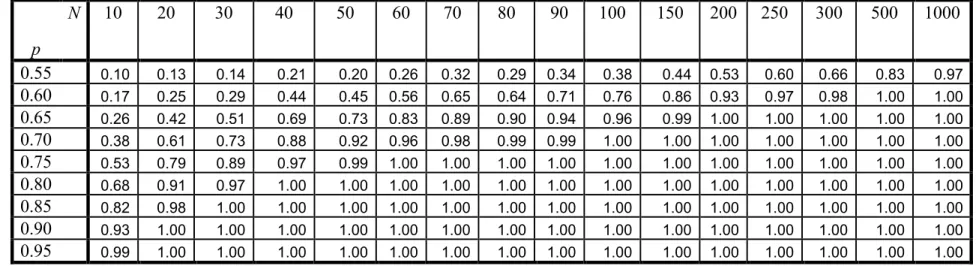
For illustration, in Table 1 in the Appendix, we provide the results on calculations of the power of the AR sign test for testing the null hypothesis H0 : P(Xn> x|=n−1) =P(Xn <−x|=n−1), x >0,

for all n against a particular case of the alternative hypothesis, namely, against the assumption that P(Xn > x|=n−1) = p > 1−p = P(Xn < −x|=n−1), x > 0, where p ∈ (1/2,1] (the power 5_{We describe the tests for the two-sided alternative since this is usually the case of interest in most of the} applications.

of other tests discussed in the present section against this particular alternative may be calculated in complete similarity). One should note that, as it is not difficult to see, the power calculations are the same for the AR test for testing H0 against the alternative P(Xn > x|=n−1) = p1 > q1 =

P(Xn < −x|=n−1), x > 0, P(Xn = 0|=n−1) = 1− p1 −q1, where p1, q1 ∈ [0,1] are such that

1/2 + (p1−q1)/2 =p. They are also the same for the AR sign test for testing the null hypothesis

of equality of conditional distributions of two (=t)−martingale differences Xt and Yt against the

alternative that P(Xt> Yt|=t−1) =p2 >1/2> q2 =P(Yt> Xt|=t−1),where p2, q2 ∈[0,1] are such

that 1/2 + (p2−q2)/6 =p. According to the table, the test has very good power properties, even

in the case of small samples.

5

Bounds in the trinomial option pricing model

In this section of the paper, we obtain sharp bounds for the expected payoffs and fair prices of contingent claims in the trinomial model with dependent log-returns.

Let{ut}∞t=1 be a sequence of nonnegative numbers and let, as before,=0 = (Ω,∅)⊆ =1 ⊆...=t⊆

...⊆ = be an increasing sequence ofσ−algebras on a probability space (Ω,=, P). Throughout the rest of the paper, we consider a market consisting of two assets. The first asset is a risky asset with the trinomial price process

S0 =s, St=St−1Xt, t≥1, (5.16)

where the (Xt)∞t=1 is an (=t)−adapted sequence of r.v.’s (additional assumptions concerning the

dependence structure of X0

ts will be made below). The second asset is a money-market account

with a risk-free rate of return r.

We assume first that random log-returns log(Xt) form an (=t)−martingale-difference sequence

and take three values ut, −ut and 0:

P(log(Xt) =ut) = P(log(Xt) = −ut) =pt, P(log(Xt) = 0) = 1−2pt, (5.17)

t ≥ 1 (so that, in period t, the price of the asset increases to St = exp(ut)St−1, decreases to

St=exp(−ut)St−1 or stays the same: St=St−1).

As before, in what follows, we denote by Et, t ≥0, the conditional expectation operator Et =

E(·|=t).6

For t ≥ 0, let ˜Sτ, τ ≥ t, be the price process with ˜Sτ = St and ˜Sτ = ˜Sτ−1exp(uτ²τ), τ > t,

where, conditionally on =t, (²τ)∞τ=t+1 is a sequence of i.i.d. symmetric Bernoulli r.v.’s.

The following theorem gives sharp estimates for the time-texpected payoff of contingent claims in the trinomial model with an arbitrary increasing convex payoff functions φ : R+ → R. These

estimates reduce the problem of derivative pricing in the multiperiod trinomial financial market model to the case of the multiperiod binomial model with i.i.d. returns.

Theorem 5.1 For any increasing convex function φ :R+→R, the following sharp bound holds:

Etφ(ST)≤Etφ( ˜ST)

for all 0≤t < T.

Proof. The theorem follows from Theorem 2.3 applied to the r.v.’s log(Xk) and the function

f(x1, ..., xT−t) = φ ³ Stexp ³_XT−t k=1 xk ´´ . ¥

The choice of the function φ(x) = max(x − K,0) in Theorem 5.1 immediately gives sharp estimates for the time-t expected payoffs of a European call option with strike price K ≥ 0 on the asset expiring at time T. Furthermore, using the results in Eaton (1974) similar to the proof of the second inequality in estimates (3.10) given by Corollary 3.3, we also obtain sharp bounds for the expected payoff of European call options in the trinomial model in terms of the expected payoff of power options with the payoff function φ(x) = [max(x−K,0)]3 _{written on a stock with}

log-normally distributed price. These bounds are similar in spirit to the estimates in the binomial model in terms of Poisson r.v.’s obtained in de la Pe˜na et al. (2004) and, essentially, reduce the problem of option pricing in the trinomial multiperiod model to the problem of contingent claim pricing in the case of two-periods and the standard assumption of normal returns.

Theorem 5.2 The following sharp bounds hold:

Etmax(ST −K,0)≤Etmax( ˜ST −K,0)≤ n Et h max ³ Stexp ¡ Z T X k=t+1 u2 k ¢ −K,0¢i3 o_1/3 , (5.18)

where, conditionally on =t, Z has the standard normal distribution.

Proof. As indicated before, the first inequality in (5.18) is an immediate consequence of Theorem 5.1 applied to the increasing convex function φ(x) = max(x−K,0). The second estimate in (5.18) follows from Jensen’s inequality and the fact that, similar to (3.12), the results in Eaton (1974) imply Et h max ³ Stexp ¡ XT k=t+1 ut²t ¢ −K,0 ´i₃ ≤Et h max ³ Stexp ¡ Z T X k=t+1 u2_k¢−K,0 ´i₃ . ¥

Bounds similar to those given by Theorems 5.1 and 5.2 hold as well for the expected stop-loss for a sum of three-value risks that form a martingale-difference sequence (the proof of the estimates for the expected stop-loss of a sum of risks is completely similar to the argument for Theorems 5.1 and 5.2).

Theorem 5.3 Suppose that the r.v.’s Xt form an (=t)−martingale-difference sequence and have

distributions

P(Xt=ut) = P(Xt=−ut) = pt, P(Xt= 0) = 1−2pt. (5.19)

Then the following sharp estimate holds for the expectation of any convex function φ : R →R of the sum of the risks Pn_t=1Xt :

Eφ¡ n X t=1 Xt ¢ ≤Eφ¡ n X t=1 ut²t ¢ .

In particular, the following sharp bound holds for the expected stop-loss Emax(Pn_t=1Xt−K,0),

K ≥0 : Emax ³_Xn t=1 Xt−K,0 ´ ≤Emax ³_Xn t=1 ut²t−K,0 ´ .

Let us now turn to the problem of making inferences on the European call option price in the trinomial model. As is well-known, the trinomial option pricing model is incomplete and allows for an infinite number of equivalent probability measures under which the discounted asset price process is a martingale. The different risk-neutral measures lead to different prices for contingent claims in the model all of which can be consistent with market prices of the primary assets. Therefore, the standard no-arbitrage pricing approach break down and, although it may be possible to calibrate the

model by getting it to match market prices and obtain reasonable prices for nontraded instruments, it cannot be used to fully hedge the exposure associated with derivative positions (see Shreve, 2004, pages 248-249).

The inequalities for the expected payoffs of contingent claims in Theorems 5.1 and 5.2 (under the true probability measure), together with estimates for the call return over its lifetime, on the other hand, provide bounds for possible fair prices of the option.

Let RS and RC denote, respectively, the required gross returns (over the periods t+ 1, ..., T)

on the underlying asset with the trinomial price process (5.16), (5.17) and on the European call option with the strike price K on the asset expiring at time T > t. The price of the call option at time t is given by Ct =RCEtmax(ST −K,0) (where the expectation is taken with respect to the

true probability measure) and, similarly, the price of the asset satisfiesSt=RSEtST.

As follows from Rodriguez (2003) (see also Theorem 8 in Merton, 1973), risk-averse investors require a higher rate of return on the call option than on its underlying asset and, therefore,

RC < RS.7Combining this with the bounds given by Theorem 5.2, we immediately obtain estimates

for the fair prices of European call options in the trinomial model. Similar bounds also hold for other contingent claims with convex payoff function; they can be obtained using Theorem 5.1 and estimates for the gross return on the contingent claims over their lifetimes.

For instance, in the case of independent returns Xt,

RS =St/EtST = ³ _YT k=t+1 EtXk ´₋₁ = n _YT k=t+1 [1 + 2(cosh(ut)−1)pt] o₋₁ ,

where cosh(x) = (exp(x) +exp(−x))/2, x ∈ R, and we thus have the following estimates for the call option prices.

Theorem 5.4 In the case of the trinomial option pricing model with risk-averse investors and independent returns Xt with distribution (5.17), the fair time-t prices of the European call option

7_{As discussed in Jagannathan (1984) and Rodriguez (2003), this result depends critically on the Rothschild and} Stiglitz (1970) definition of risk. Grundy (1991) provides an example in which the expected return on the option is less than the risk-free rate; however the conditiondC(S)/dS <0 in the example conflicts with theoretical models and empirical findings, see Rodriguez (2003).

on the asset satisfy the following bounds: Ct≤ n _YT k=t+1 [1 + 2(cosh(ut)−1)pt] o₋₁ Etmax( ˜ST −K,0)≤ n _YT k=t+1 [1 + 2(cosh(ut)−1)pt] o₋₁n Et h max ³ Stexp ¡ Z T X k=t+1 u2 k ¢ −K,0¢i3 o_1/3 , (5.20)

where, conditionally on =t, Z has the standard normal distribution.

6

Bounds for Asian options

The approach presented in the previous section also allows one to obtain sharp bounds for the expected payoffs and fair prices of path-dependent contingent claims in the trinomial model. As an illustration, in the present section, we derive sharp estimates for the expected payoffs of Asian options written on an asset with the trinomial price process. Bounds in the case of other path-dependent contingent claims may be derived in complete similarity to the results in this section of the paper.

Let t ≤ T −n, T > n. Consider an Asian call option with strike price K expiring at time

T written on the average of the past n prices of the asset with price process (5.16). The time-t

expected payoff of the option is

Etmax "à T X i=T−n+1 Si ! /n−K,0 # =Etmax " St à T X i=T−n+1 Xt+1...XT−nXT−n+1...Xi ! /n−K,0 # .

Using the convexity of the payoff function of the Asian option, the results given in Theorem 2.3 imply, similar to the proof of Theorems 5.1-5.3, the following bounds for the trinomial Asian option pricing model.

Theorem 6.1 If the log-returns log(Xt) form an (=t)−martingale-difference sequence and have

Etmax "à _T X i=T−n+1 Si ! /n−K,0 # ≤ Etmax " St à _T X i=T−n+1 exp( i X k=t+1 uk²k) ! /n−K,0 # . (6.21)

Estimate (6.21) simplifies in the case of an Asian option written on an asset whose gross returns form a three-valued martingale-difference sequence (so that the model represents the trinomial financial market with short-selling where the gross returns can take negative values).

Theorem 6.2 If the returns (Xt) form an (=t)−martingale-difference and have the distribution

(5.19), then the expected payoff of the Asian option satisfies the inequality

Etmax "à _T X i=T−n+1 Si ! /n−K,0 # ≤Etmax " St à _T X i=T−n+1 i Y k=t+1 uk²i ! /n−K,0 # . (6.22)

Proof. Bound (6.22) follows from Theorem 2.3 and the fact that, by Theorem 2.1, the r.v.’s

ηt =²1²2...²t are i.i.d. symmetric Bernoulli r.v.’s. ¥

References

Adler, R. J., F. R. E. and Gallagher, C. (1998), Analysing stable time series, in R. J. Adler, R. E. Feldman and M. S. Taqqu, eds, ‘A Practical Guide to Heavy Tails’, Birkhauser, Boston, pp. 113–58.

Axtell, R. L. (2001), ‘Zipf distribution of u.s. firm sizes’, Science 293, 1818–1820.

Azuma, K. (1967), ‘Weighted sums of certain dependent variables’, Tˆohoku Mathematical Journal

4, 357–367.

Boyle, P. B. and Lin, X. S. (1997), ‘Bounds on contingent claims based on several assets’, Journal of Financial Economics 46, 383–400.

Boyle, P. P. (1988), ‘A lattice framework for option pricing wuth two state variables’, Journal of Financial and Quantitative Analysis 23, 1–12.