Vortex Extraction Of Vector Fields

(1)

D

ISSERTATION

SUBMITTED

TO THE

COMBINEDFACULTIES FOR THENATURAL SCIENCES AND FOR MATHEMATICS

OF THE

RUPERTO–CAROLA UNIVERSITY OFHEIDELBERG, GERMANY FOR THE DEGREE OF

DOCTOR OF NATURALSCIENCES

Put forward by

Dipl.–Mat, M.Sc. Dorotea Dudaˇs Born in: Osijek, Croatia

(2)

(3)

Vortex Extraction Of Vector Fields

Advisors: Prof. Dr. Rolf Rannacher

PD Dr. Christoph S. Garbe

(4)

(5)

Abstract

Spinning, turbulent structures swirling around its centers within various flow me-dia are known as vortices. The capability of locating and extracting vortical struc-tures in flow data is crucial for understanding the flow. Vortices also have a strong impact on flow control and transport processes.

Real-time vortex extraction methods are presented, offering immediate no-tion of the shape and locano-tion of the vortex structures. Using a real-time fluid simulation based on Navier-Stokes equations presented in [46], several vortex traction methods are interactively performed in real-time. Following vortex ex-traction methods are implemented using the GPU: vorticity threshold, Q criterion, λ2 criterion, the eigenvector method via parallel vectors operator (PVO) and the

eigenvector method via coplanar vectors operator (CVO).

Diffusional methods outputting flow fields with preserved/enhanced vortical structures are also presented. Such methods are useful for obtaining an alternative insight into vortices within a flow field and can also be used within the real-time simulation.

Using a number of human performed gestures for human-computer interac-tion, special ensemble flow fields are produced. Detecting vortices from these gesture ensemble range flows is introduced as aid for gesture classification. Ges-ture range data is recorded using the Microsoft Kinect device. Range or scene flow is a 3D vector field describing movement within a scene. Range data con-sists of images (color channels) and corresponding depth images (depth channels) in which the distance of objects is recorded as a grayscale image. Ensemble range flow is estimated from gesture videos. Ensemble flow describes the overall flow within the scene and is obtained by averaging the structure tensor throughout the scene. Vortices are extracted from an ensemble range flow of the gestures. Their

(6)

number and location is offering an additional parameter for gesture classification. Collection of methods for detecting vortices and obtaining vector fields with emphasized vortices are introduced in this thesis. Real-time execution of vortex extraction methods offers an instant notion of the nature of the flow. Diffusional methods can serve as a processing step within the real-time vortex extraction. As an additional application, gesture ensemble flow is presented. By detecting its vortices, a parameter for gesture classification is introduced.

(7)

Zusammenfassung

In einer Strömung werden rotierende, turbulente Strukturen, die sich um ein Zen-trum drehen als Wirbel bezeichnet. Deren Charakterisierung und Lokalisierung ist essentiell für das Verständnis einer Strömung. Weiterhin haben Wirbel einen bedeutenden Einfluss auf das Verhalten einer Flüssigkeit und Transportprozesse innerhalb der Flüssigkeit.

Hier werden Methoden für die Extraktion von Wirbeln in Echtzeit vorgestellt, die die sofortige Ansicht von Ort und Form der Wirbelstruktur ermöglichen. Mehrere Wirbelextraktionsmethoden werden interaktiv und in Echtzeit ausgeführt und Daten aus einer Simulation der Navier-Stokes-Gleichungen in Echt-zeit ([46]) angewendet. Dabei handelt es sich um folgende Methoden: Vortizitäts-schwellwert, Q Kriterium, λ2 Kriterium, Eigenvektorenmethode über parallele

Vektoroperatoren (PVO) und Eigenvektorenmethode ¨uber Koplanare Vektoroper-atoren (CVO).

Weiterhin werden auf Diffusionsprozessen basierte Methoden zur Gener-ierung von Strömungsfeldern präsentiert mit erhaltenen/verstärkten turen. Diese Methoden ermöglichen einen alternativen Einblick in Wirbelstruk-turen innerhalb des Geschwindigkeitsfeldes und können auch in der Echtzeitsim-ulation eingesetzt werden.

Ensemble Geschwindigkeitsfelder wurden von einer Auswahl menschlicher Gesten im Rahmen der Mensch-Computer-Interaktion generiert. Die Vortexde-tektion aus diesen gesteninduzierten Geschwindigkeitsfeldern wird als Hilfe in der Gestenklassifikation vorgestellt. Die nötigen Daten wurden mit der Mi-crosoft Kinect Kamera aufgenommen. Das aufgenommene Geschwindikeits-feld ist ein 3D VektorGeschwindikeits-feld, das die Bewegung innerhalb eine Szene beschreibt. Die zugehörigen Daten bestehen aus 3-Kanal Farbbildern und dazugehörigen

(8)

Tiefenkarten, in denen der Abstand der Objekte als Grauwertbild gespeichert wird. Ein Ensemble Geschwindigkeitsfeld wird aus jedem Gestenvideo berech-net. Es beschreibt die durchschnittliche Bewegung und wird durch die Mittelung des Strukturtensors über die gesamte Szene bestimmt. Im Anschluss werden die Wirbel aus den resultierendenEnsembleGeschwindigkeitsfeldern bestimmt. Ort und Anzahl der Wirbel stellen einen zusätzlichen Parameter für die Gestenklassi-fikation dar.

In dieser Arbeit wird eine Auswahl von Methoden zur Detektion von Wirbeln und Erzeugung von Vektorfeldern mit Schwerpunkt auf Wirbeln vorgestellt. Die Ausführung der Methoden der Wirbelextraktion in Echtzeit ermöglicht die so-fortige Kenntnis der Art des Geschwindigkeitsfeldes. Die Anwendung der Dif-fusionsmethoden kann einen Schritt innerhalb der Vortexextraktion in Echtzeit darstellen. Als eine zusätzliche Anwendung wird die Generierung von Ensem-ble Geschwindigkeitsfeldern aus Gesten vorgestellt. Uber die Detektion der¨ entstehenden Wirbel wird ein zusätzlicher Parameter für die Gestenklassifikation eingeführt.

(9)

Chapter 1 Introduction

Due to extreme climatic changes, importance of understanding vortices increases. Figure 1.1 shows different instances of vortical structures.

Figure 1.1: Vortices. Upper, left: World tallest artificial tornado serving as a smoke draining system in Mercedes-Benz museum in Stuttgart ([23], Copyright Daimler AG). Upper, right: Tornado storm in the “tornado alley” area in the central USA (Orchard, Iowa, June 2008 [25]). Lower: A fire tornado near Alice Springs, Australia (Sep, 18. 2012 [4]).

A collection of methods for detecting vortices and obtaining vector fields with emphasized vortices are introduced in this thesis. Real-time vortex extrac-tion methods are presented, offering immediate noextrac-tion of the shape and locaextrac-tion

(14)

Introduction 2 of the vortex structures. Diffusional methods outputting flow fields with pre-served/enhanced vortical structures are also introduced. Detecting vortices from gesture ensemble range flows is introduced as a possible application of the devel-oped methods to gesture classification.

Chapter 2 Chapter 2 is an introductory chapter presenting some of the back-ground knowledge necessary for understanding the other chapters. Obtaining flow data, whether by designing analytical flow fields, by simulating the flow or by recording the flow, is crucial for the study of vortices. Chapter 2 is divided into sections on simulated (Section 2.2) and recorded data (Section 2.3).

Section 2.2 on simulated data is divided into “Analytical Vortex Examples” (Section 2.2.1) and “Real-Time Flow Simulation on the GPU” (Section 2.2.2) sections.

For designing analytical vector fields suitable for studying vortices, it is nec-essary to have some knowledge about the vector field topology. Certain types of first order critical points are considered to be vortex cores in 2D. Analytical 2D flow fields containing such critical points, i.e. vortex cores, are extensively used to test diffusion and diffusion-reaction processes in Chapter 3. Analytical 3D flows are designed to test 3D extraction methods presented in Chapter 4. Eigen-vector method for vortex extraction ([47]) is a standard vortex extraction method. To understand where the motivation for its design originated from, first order 3D critical points are presented. Parallel vectors operator method, extensively used in Chapter 4, was motivated by the eigenvector method.

Simulating fluid in real-time is presented in Section 2.2.2. Using this fluid simulation in Chapter 4, vortex extraction methods are implemented in real-time. The simulation is based on Navier-Stokes equations which describe the motion of fluid substances. Implementation was done on a GPU using the CUDA frame-work. Interactive 3D real-time fluid simulation allows user to input additional force into the data volume, so creating flow data in real-time.

Section 2.3 presents the range data used in Chapter 5 for detecting vortices withing the gesture flow. The data is recorded using the Microsoft Kinect device. The device has a standard camera and an infrared sensor that records the depth information. Range data consists of images (color channels) and corresponding

(15)

Introduction 3 depth images (depth channels) in which the distance of objects is recorded as a grayscale image. Such range data is used to create the ensemble range flow (Section 5.4) used for classifying gestures (Section 5.5).

Chapter 3 Chapter 3 presents diffusion and diffusion-reaction (variational) pro-cesses which produce vector fields with preserved/emphasized vortices.

Sections 3.2 and 3.3 give an introduction into diffusional and variational pro-cessing framework. Basic diffusion and diffusion-reaction processes are presented in order to facilitate the understanding of the upcoming sections.

Vortex preserving diffusion and variational processes are presented in Section 3.4.

Vortex preserving diffusion (Section 3.4.1) results in vector fields with pre-served vortex areas where rest of the flow field is dampened. Diffusion produces simplified and information-reduced output. By choosing diffusivity functions that avoid vortex areas, diffusion processes are steered to preserve the information within them. Other features are diminished. It is also preferred, but not guaran-teed that no new features are created. Different binary and continuous diffusivity functions are designed. One choice for designing diffusivity functions is making them dependent on the discriminant dof the characteristic polynomial of the Ja-cobian matrix. Negatived indicates an existence of a swirling area that possibly contains swirling critical points i.e. critical points that can be classified as vor-tex cores in 2D. Other choice for diffusivity functions includes considering area around detected vortex cores or regions. All approaches output vector fields with emphasized vortex areas.

Variational processes which give vector fields with emphasized/preserved vor-tex areas are presented in Section 3.4.2. A function H that causes preservation of certain areas and destruction of others is used to preserve vortices. His again steered either by discriminantd, or by the areas around vortex cores or regions.

Designed processes offer an alternative insight into the structure of the flow and are useful for the further study of vortices.

(16)

Introduction 4

Chapter 4 Chapter 4 presents real-time vortex detection and extraction meth-ods. Various vortex core and region extraction methods exist. They operate as a post-processing step for locating vortex regions/cores. Here, standard vortex extraction methods are performed in real-time and are implemented within the real-time fluid simulation based on Navier-Stokes equations (presented in Section 2.2.2).

Overview of the vortex extraction methods is given in Section 4.2. Vortex core and region extraction methods needed for testing or for real-time implementation are covered. Following vortex region detection methods are presented: vorticity threshold, Q criterion and λ2 criterion. Vortex core extraction includes minimal

bending energy vortex extraction, the eigenvector method and the parallel vector operator (PVO). Eigenvector method is one of the standard vortex core extrac-tion methods and is a predecessor of the PVO. Coplanar vectors operator (CVO) method, which is a generalization of the PVO, can be expressed through PVO.

GPU implementation of the parallel vectors operator method (PVO) for sta-tionary vector fields is presented in Section 4.3. OpenCL framework is used for programming. PVO is used as a testing method for vortex extraction from 3D vec-tor fields obtained by pausing the real-time simulation. This way, it is possible to verify the results from the real-time extraction. GPU implementation is optimized by considering only limited amount of faces within a volume cell of the 3D data.

Section 4.4 introduces real-time vortex core/region extraction. CUDA is used as a programming environment. Extraction methods are implemented within a real-time fluid simulation which is interactively influenced by the user. User is able to input additional force into the flow field in real-time (see Section 2.2.2) and so form, e.g. a helical-like flow suitable for testing of the real-time extrac-tion methods. The results of the real-time extracextrac-tion are color coded within the arrow or within the density plot of the real-time simulation. Different extraction methods can be compared in real-time by using different colors to depict them. Following vortex extraction methods are implemented: vorticity threshold, Q cri-terion, λ2 criterion, the eigenvector method via parallel vectors operator (PVO)

and the eigenvector method via coplanar vectors operator (CVO). Vortex preserv-ing diffusion methods presented in Section 3.4.1, can be used as a replacement for the diffusion step of the fluid simulation, producing flows with slightly

(17)

empha-Introduction 5 sized swirling areas.

Chapter 5 Chapter 5 deals with detecting vortices within the ensemble range flow of the gesture videos. The designed method is intended as a improvement of the existing gesture classification methods.

Section 5.2 is an introductory section presenting basics of optic and range flow. Range or scene flow is a 3D vector field describing movement within a scene. It requires image pairs of color images and of depth images as input. Depth images are encoding the distance of objects in an observed scene using grayscale values. Data recorded with Kinect device is used for testing.

Depth data obtained by Kinect contains many artifacts. Section 5.3 introduces a range flow method that removes those artifacts. Improved global-local range flow algorithm is presented. Magnitude of the derivatives of the input depth im-ages is thresholded, thus removing the influence of artifacts to the resulting flow.

Ensemble range flow is introduced in Section 5.4. It describes the overall flow within the considered scene. The structure tensors of images are averaged throughout the entire data set.

Section 5.5 shows how vortex detection of the gesture ensemble range flows can aid gesture classification. Five volunteers recorded nine gestures using the Mi-crosoft Kinect device. Ensemble range flow is calculated for every gesture. Vortex cores extracted from these ensemble range flows, i.e. their position and number can serve as a addition to certain gesture classification methods. Although this approach can be used as a standalone indicator, it is intended as an improvement of gesture classification methods that operate on data of reduced dimensions. A draft for a newly designed gesture classification is also proposed. The technique is based on mapping of the ensemble range flow magnitudes to 1D, so allowing fast classification. Gesture classification requires only the number of obtained vor-tices. Diffusion techniques from Section 3.4.1 can be used to create a flow field with emphasized vortices.

Appendix Different mathematical formulations leading to discrete explicit schemes are presented in Appendix A. Calculation of the ensemble range flow of the fluid data by estimating the depth data is given in Appendix B.

(18)

(19)

Chapter 2 Flow Data

2.1 Introduction

In order to deal with flow data, it is important to understand its origin and basic topological structure. Different approaches for obtaining flow data as well as some theoretical background of the flow topology and flow simulation are presented in this chapter.

2D flow fields and their topology are presented in order to better understand diffusion and diffusion-reaction processes covered in chapter 3. Since only certain types of first order critical points are considered to be vortex cores, the ability to recognize such features is essential for their processing and extraction. During an iterative process on a 2D vector field, two critical points sometimes collapse into one, or vice versa. These special events are called bifurcations and should also be considered when dealing with 2D flow data.

In order to understand where the idea for the 3D eigenvector vortex extraction method came from, one should also be familiar with first order 3D critical points. If 3D critical points of the saddle focus type are considered, the direction of the vortex core coincides with the direction of the only “real eigenvector” of the Ja-cobian matrix of that point. The eigenvector method led to the development of the parallel vectors operator used in chapter 4. 3D vector fields specially designed to test vortex extraction methods, such as a helical flow field or bent helical flow field are also presented.

(20)

Simulated Data 8 Real-time fluid simulation, used in Chapter 4 to implement and test the real-time vortex extraction methods, is based on simulating the Navier-Stokes equa-tions. These partial differential equations describe the motion of fluid substances. The real-time simulation, and later the vortex detection methods, are implemented on the GPU using the CUDA framework. Parallel vector operator for stationary fields is also implemented on the GPU using the OpenCL framework.

Range flow methods developed in chapter 5 rely on data recorded using spe-cial equipment, e.g. Microsoft Kinect device. Such devices produce not only color video sequences, but also, by utilizing an infrared projector, provide depth sequences i.e. data that contains information about distance of objects to the de-vice.

Section 2.2 gives some insights into simulation of the flow data. Analytical examples are presented in Section 2.2.1. Section 2.2.1.1 gives an introduction into the vector field topology important for understanding the structure of the flow. Simulating flow in real-time using the graphic processing units (GPUs) is covered in Section 2.2.2. Section 2.2.2.1 explains the governing Navier-Stokes equations. Section 2.2.2.2 reveals some details of the simulation implementation.

Section 2.3 is about the acquisition of the flow data. Acquisition of range data using the Microsoft Kinect is covered in Section 2.3.1.

The vector field data, techniques and theories presented here are used throughout the rest of the thesis.

2.2 Simulated Data

Simulated flow data in the thesis is produced by using 2D and 3D analytical flow examples or by simulation of the Navier-Stokes equations.

(21)

Simulated Data 9

2.2.1 Analytical Vortex Examples

In order to test vortex extraction methods or design processes that preserve vor-tices, it is necessary to have analytical examples for which the exact solution of the given problem is known. Producing such examples requires certain knowledge about the main features of the vector field i.e. about its topology.

2.2.1.1 Vector Field Topology

First Order Critical Points The main feature of a vector field are its critical points. Definition of a first order critical point is given as: x0 is a first order critical point of the vector field v(x)if and only ifv(x0) = 0and |J(x0)| 6= 0, whereJis the Jacobian matrix of the flow in a point.

Figure 2.1: First order critical points in 2D linear vector field.

The flow pattern in a 2D vector field around the critical point is characterized by eigenvalues and eigenvectors of the Jacobian matrix in that point and can be

(22)

Simulated Data 10 classified (Figure 2.1) as:

repelling node : 0< Re(λ1)< Re(λ2) , Im(λ1) = Im(λ2) = 0, attracting node : Re(λ1)< Re(λ2)<0 , Im(λ1) = Im(λ2) = 0, saddle point : Re(λ1)<0< Re(λ2) , Im(λ1) = Im(λ2) = 0, repelling focus : 0< Re(λ1) =Re(λ2) , Im(λ1) = −Im(λ2)6= 0, attracting focus : Re(λ1) = Re(λ2)<0 , Im(λ1) = −Im(λ2)6= 0, center : 0 = Re(λ1) =Re(λ2) , Im(λ1) = −Im(λ2)6= 0.

First order critical points in 2D can therefore be divided into a saddle points, nodes, foci and centers. Repelling node and focus can also be called sources, while attracting node and focus are also called sinks. If eigenvalues are imaginary numbers then the critical point (focus or center) can be characterized as a vortex i.e. a swirling critical point.

Separatrices Next to critical points, separatrices are also significant features of the flow. Separatrices are streamlines that separate regions of different flow behavior. In parabolic region all tangent curves originate or end in the critical point. In hyperbolic region all tangent curves go by the critical point, except the two that end/begin in it. In elliptic sector all tangent curves originate and end in the critical point. Each streamline that starts/ends in a critical point which separates two sectors is a separatrix. Special cases of isolated streamlines and stream lines through boundary switch points are also separatrices.

Bifurcations Sudden changes of flow structure at a certain time are called bifurcations. Fold bifurcations is an event where a saddle collapses with a source/sink/center and both of them disappear (Figure 2.2) or a reversed process. Visualizations were made using the Mathematica toolkit ([21]). Hopf bifurcation is switching of the repelling node to an attracting node via center or reversed. Saddle connection is another type of the bifurcation where a separatrix of one saddle ends in a separatrix of another saddle. Collapsing of the separatrix of a saddle into the same saddle is called a blue sky bifurcation. Cyclic fold bifurcation is collapsing of two isolated closed streamlines into each other.

(23)

Simulated Data 11

Figure 2.2: Four stages of a fold bifurcation. A saddle and a center col-lapse into each other and disappear with vector fields ranging from u(x, y) = y2−0.25 −x tou(x, y) = y2+ 0.25 −x .

2D Examples Analytical models containing a single critical point are easiest to consider for testing purposes. Jacobian matrices producing respectively saddle, attracting node, repelling node, center, attracting focus, repelling focus are:

1 0 0 −1 ! , −1 0 0 −1 ! , 1 0 0 1 ! , 0 1 −1 0 ! , 0 1 −1 −1 ! , 0 1 −1 1 ! . (2.1)

Following the fact that linear 2D or 3D vector fields can be simplified asv=Jx

(where xis a 2D/3D vector andJ a constant Jacobian matrix of the flow field), the corresponding vector fields are:

x −y ! , −x −y ! , x y ! , y −x ! , y −x−y ! , y −x+y ! . (2.2)

Creating vector fields with several critical points is also useful for testing different methods (Figure 2.3).

(24)

Simulated Data 12

(a) (b) (c) (d)

Figure 2.3: Creating a 2D vector field by sampling the analytical function: (a) u(x, y) = y −x , (b) u(x, y) = y2₋₀_.₂₅ −x , (c) u(x, y) = x2₋₀_.₂₅ y2₋₀_.₂₅ , (d) u(x, y) = y2₋₀_.₂₅ x2₋₀_.₂₅ .

3D First Order Critical Points 3D topology is more complicated to consider. In 3D classification of the first order critical points is as follows:

sources : 0< Re(λ1)≤Re(λ2)≤Re(λ3),

repelling saddles : Re(λ1)<0< Re(λ2)≤Re(λ3),

attracting saddles : Re(λ1)≤Re(λ2)<0< Re(λ3),

sinks : Re(λ1)≤Re(λ2)≤Re(λ3)<0.

Each of the four cases is subdivided by considering the imaginary parts:

foci : Im(λ1) = 0, Im(λ2) =−Im(λ3)6= 0,

nodes : Im(λ1) = Im(λ2) = Im(λ3) = 0,

where λ1, λ2, λ3 are the eigenvalues of the Jacobian matrix. Figure 2.4 shows

some of the possible first order 3D critical points. Critical points containing a vortex are the ones with two conjugated complex eigenvalues that have opposite signs of real parts when compared to the third eigenvalue i.e. focus saddles. In critical points of the focus saddle type the direction of the vortex core coincides with the direction of the only “real eigenvector” of the Jaco-bian matrix of that point. The eigenvector method for vortex extraction, which led to the parallel vectors operator, is a generalization of that fact to the entire flow.

(25)

Simulated Data 13

(a) (b) (c) (d)

(e) (f) (g) (h)

Figure 2.4: First order 3D critical points: (a) source node, (b) repelling saddle node, (c) attracting saddle node, (d) sink node, (e) source focus, (f) repelling saddle focus, (g) attracting saddle focus, (h) sink focus.

3D Examples Jacobian matrices producing respectively (Figure 2.4): source node, repelling saddle node, attracting saddle node, sink node, source focus, re-pelling saddle focus, attracting saddle focus, sink focus are e.g.:

   1 0 0 0 1 0 0 0 1   ,    1 0 0 0 1 0 0 0 −1   ,    1 0 0 0 −1 0 0 0 −1   ,    −1 0 0 0 −1 0 0 0 −1   ,    0 1 0 −1 1 0 0 0 1   ,    0 1 0 −1 1 0 0 0 −1   ,    0 1 0 −1 −1 0 0 0 1   ,    0 1 0 −1 −1 0 0 0 −1   , (2.3)

with corresponding flow fields being:

(x, y, z)T, (x, y,−z)T, (x,−y,−z)T, (−x,−y,−z)T,

(26)

Simulated Data 14

(a) (b) (c)

Figure 2.5: Side and front view of the 3D helical vector field. Visualizations were made using the ParaView scientific visualization application ([29]).

Some other common examples of 3D vector fields used for testing are the fol-lowing. In 2D a center can also be considered as a velocity field of a solid body rotation. Its Jacobian matrix is:

0 −ω

ω 0

!

, (2.5)

whereω is a rotational speed of the rotation of the solid body around the origin. When a constant motion perpendicular to the 2D rotation plane is added ahelical flow field(Figure 2.5) is obtained. Its Jacobian matrix is:

   0 −ω 0 ω 0 0 0 0 γ   , (2.6)

where γ is the speed of the constant motion perpendicular to the rota-tion plane. Using the speed zero the following vector field is obtained

(27)

Simulated Data 15

Figure 2.6: Circular helical vector field. Upper row: Side and front view of the bent helical vector field with circular vortex core. Lower row: Side and front view of the bent helical vector field with circular vortex core - a closer look at the streamlines around the core.

In order to construct a bent helical vector field with circular vortex ([37]) (Figure 2.6), a helical vortex is translated and bent around an axis resulting in a following vector field: v=         −ωxzR r2 − Ωy r −ωyzR r2 + Ωx r R− R 2 r ω         ,

wherer=px2 ₊_y2_{. The vortex core is a circle of radius}_R_{around the}_z _axis. _ω

is the rate of the rotation around the core,Ωis the large-scale rotation around the z axis.

(28)

Simulated Data 16

(a) (b)

Figure 2.7: Side and front view of a helical vortex with core dislocated fromz=−1to

z= 1via a blending function. The dislocated core is clearly visible in Figure (b).

Helical vortex with “dislocated” core (Figure 2.7) is constructed by using:

v=    y+f(z) −x 1   , (2.7) where function f(z) =      −1, z <−1 x, −1≤z ≤1 1, z >1 (2.8)

is added to one vector field component, such that a vortex core is dislocated away from the plane center by the value of −1on one side of the spiraling plane, and value of 1 on the other side of the plane, except “near” the center, according to f(z).

2.2.2 Real-Time Flow Simulation on the GPU

Vortex extraction methods are incorporated within a real-time simulation of the flow in Chapter 4. Real-time simulation is implemented by following the paper “Stable Fluids” [46]. It is based on simulating the Navier-Stokes equations.

(29)

Simulated Data 17

2.2.2.1 Navier-Stokes equations

Navier-Stokes equations are a set of differential equations that describe the mo-tion of fluid substances. The Navier-Stokes equamo-tion for incompressible flow of Newtonian fluids in vector form is:

ρ ∂v ∂t + (v· ∇)v =−∇p+µ∇2_v₊_f_, (2.9) where ρ is the density of flow medium, µ dynamic tenacity, p pressure and f

represents body forces such as gravity or centrifugal force. The meaning of the individual terms in the equation (2.9) is the following:

ρ ∂v ∂t + (v· ∇)v inertia, ∂v ∂t unsteady acceleration, (v· ∇)v convective acceleration, −∇p+µ∇2_v _{divergence of stress,} −∇p pressure gradient, µ∇2_v _viscosity, f other forces. (2.10)

The incompressible Navier-Stokes equation (2.9) is a differential algebraic equation (DAE) which has no explicit mechanism for advancing the pressure in time. It is desired for pressure to be eliminated from the equations and thus create a pressure-free Navier-Stokes velocity formulation.

Helmholtz decomposition states that any sufficiently smooth, rapidly decay-ing vector field in three dimensions can be resolved into the sum of an irrotational (curl-free) vector field and a solenoidal (divergence-free) vector field. The incom-pressible Navier-Stokes equation (2.9) can be written as a sum of two orthogonal equations, a pressure-free governing equation for the velocity (2.11) and a

(30)

func-Simulated Data 18 tional of the velocity related to pressure Poisson equation (2.12):

∂u ∂t = Π S ₋ (u· ∇)u+µ∇2u+fS, (2.11) ρ−1∇p = ΠI −(u· ∇)u+µ∇2_u +fI, (2.12) where areΠS_,_ΠI _{are solenoidal and irrotational projection operators with}_ΠS₊

ΠI = 1, and are fS, fI the nonconservative and conservative parts of the body force.

Pressure-free Navier-Stokes equation is used to implement the real-time fluid simulation.

Real-Time Fluid Simulation The real-time fluid simulation method presented in paper Stable Fluids [46] was initially designed to move the density particles along a stationary vector field (Figure 2.8). Particles are influenced by the addi-tional density inputed into a density scalar field, they are moved into the direction of the vector field and also there is a certain amount of diffusion (dissipation) happening.

Figure 2.8: Advection i.e. moving of the density (denoted white) through the static vector field (denoted by a blue arrow plot) ([46]).

Pressure-free Navier-Stokes equation for velocity that governs such behavior is given as:

∂u

∂t = P

−(u· ∇)u+µ∇2u+f, (2.13) with projection operator P that projects a vector field onto its divergence-free component. The following notation for density and velocity equations shall be

(31)

Simulated Data 19 used for simplicity:

∂ρ ∂t = −(u· ∇)ρ+κ∇ 2 ρ+S, (2.14) ∂u ∂t = −(u· ∇)u+µ∇ 2 u+f, (2.15)

whereρis the density,uvector field,Sadditional density,fadditional force. The meaning of the individual terms in the equation (2.14) is the following:

−(u· ∇)ρ movement along the vector field, κ∇2_ρ

diffusion of the density,

S input of additional density.

(2.16)

Similar equation is also used for velocity (2.15), where individual terms can be interpreted as:

−(u· ∇)u self-advection, µ∇2u viscous diffusion,

f additional forces.

(2.17)

A simulation of a swirling divergence free (without sources or sinks) vector field was accomplished in the following way. As already mentioned, every velocity field can via Helmholtz decomposition be represented as a sum of a divergence free field and a gradient field. We want to project a vector field onto its divergence free part containing no sinks or sources, but containing many swirls (Figure 2.9). The projection onto a divergence free space is achieved by subtracting the gradient field from the original vector field. The gradient field is obtained by solving a Poisson equation (2.19).

2.2.2.2 Implementation

Fluid simulation runs in real-time and has a scalable flow field grid. By using a right mouse click the user can input a desired amount of density into the plane (in 2D) or first slice of the volume (in 3D). Left mouse click adds forces to the vector field (first slice of the vector field in 3D). The forces spread the density around

(32)

Simulated Data 20

= +

= –

Figure 2.9: Upper row: original vector field is decomposed into a mass conserving field and a gradient field. Lower row: by subtracting the gradient field from the original field we get the visually appealing divergence free field ([46]).

the volume (Figure 2.10). The view can be switched between an arrow plot and the density plot of the vector field. Pseudo-volume rendering i.e. rendering of transparent textures is used to visualize the density of the volume. Simulation is needed in order to test the real-time performance of the vortex extraction methods presented in chapter 4. Quantities indicating a vortex are visualized instead of density. It is possible to pause a simulation and save a stationary flow data. Data can also be saved in regular time periods thus producing a 3D time dependent data.

(a) (b) (c) (d)

Figure 2.10: 2D and 3D real-time fluid simulation. (a) 2D simulation, arrow plot of the vector field, (b) 2D simulation, density (denoted blue) plot, (c) 3D simulation, arrow plot of the vector field (sphere is to test the camera movement and not related to the simulation), (d) 3D simulation, density (denoted cyan) pseudo-volume.

(33)

Simulated Data 21

Implementation Detail Starting point of the implementation is a 2D C code provided by the author of a Stable Fluid paper ([46]). The code was expanded to a 3D CUDA GPU version. The finite grid size is set. The solver is started with an initial state of density and velocity which are then updated according to the environment and newly inputed density/forces. Simulation is based on four functions: source input, diffusion, advection and projection acting as follows:

• Source input adds additional density into the density field or additional forces into the velocity field. The adding of the forces is preformed by the user by using the mouse pointer movement.

• Diffusion procedure is a stable backward diffusion process (given in Ap-pendix A.4) that results in a sparse linear system solved by using a Gauss-Seidel relaxation (2.25).

• Advection procedure forces density/velocity to follow a given velocity field. Linear backtracing is used to trace particles back in time. The new den-sity/velocity value it then obtained by bi/trilinear interpolation. Trilinear interpolation is an extension of linear interpolation to 3D (Figure 2.11):

v(x, y, z) = (1−x)(1−y)(1−z)v0,0,0+x(1−y)(1−z)v1,0,0

+ (1−x)y(1−z)v0,1,0+ (1−x)(1−y)zv0,0,1

+xy(1−z)v1,1,0+ (1−x)yzv0,1,1

+x(1−y)zv1,0,1+xyzv1,1,1.

(2.18)

Figure 2.11: Trilinear interpolation of the vector fieldvin a 3D cell. The value of the flow field at the location of the red “point” is obtained using (2.18).

(34)

Simulated Data 22 • Projection routine forces velocity field to be mass conserving. Visually it produces a swirly flow without sources or sinks. Mass conserving i.e. diver-gence free vector field is obtained by subtracting the gradient field from the original vector field. The gradient field is obtained by solving the Poisson equation:

∆u=f. (2.19)

Poisson equation is a large sparse linear system. For example, in 2D the equation (2.19) is rewritten as:

f = ∂xxu+∂yyu, (2.20)

f = ui+1,j−2ui,j+ui−1,j

h2 +

ui,j+1−2ui,j+ui,j−1

h2 , (2.21)

h2f = ui+1,j+ui−1,j+ui,j+1+ui,j−1−4ui,j, (2.22) and yields a systemAu=b, where a system matrix is of the form:

A=               D −I 0 · · · 0 −I D −I 0 · · · 0 0 −I D −I 0 · · · 0 .. . . .. ... ... ... ... ... 0 · · · 0 −I D −I 0 0 · · · 0 −I D −I 0 · · · 0 −I D               , (2.23)

whereIis the identity matrix, andDof the following form:

D=               4 −1 0 · · · 0 −1 4 −1 0 · · · 0 0 −1 4 −1 0 · · · 0 .. . . .. ... ... ... ... ... 0 · · · 0 −1 4 −1 0 0 · · · 0 −1 4 −1 0 · · · 0 −1 4               . (2.24)

(35)

Simulated Data 23 The Poisson equation is solved by using a red-black Gauss-Seidel scheme:

uk_i,j+1 = u k i+1,j+uki−+11,j+u k i,j+1+uki,j+1−1 4 − h2f 4 (2.25)

Red-black denotes an alternating usage of pixel grid in each iteration i.e. a grid is divided into a red-black chess-like pattern and only red or only black pixels are used in one iteration.

These four routines combined produce a fluid simulation. Density is simulated by iteration of adding additional density, diffusing and advecting. Velocity is sim-ulated by iteration of adding force, diffusing, advecting, projecting. Boundary conditions are set so that the velocity component perpendicular to the cell bor-der is zero. The routines are implemented as CUDA kernels operating in parallel on GPU. OpenGL was used for visualization of vector field/density/vortex mea-sures. Additional GPU routines are implemented for vortex extraction in Chapter 4. They are visualized by connecting the vortex indicators to the color of the volume/arrow plot.

CUDA Implementation and Optimization The simulation is implemented by using OpenGL and nVidia CUDA and is running on the GPU. nVidia CUDA (Compute Unified Device Architecture) is a parallel computing architecture developed by nVidia for graphics processing. C for CUDA (C with nVidia extensions and certain restrictions) is used to code algorithms for execution on the graphics processing units (GPUs). The main feature of using CUDA (or OpenCL) is the ability of parallel computation on many cores allowing very large speedups if used properly.

Optimizing code for GPU requires certain knowledge about the hardware ar-chitecture and is sometimes contraintuitive. Main opportunities for optimization (other than changing the algorithm) lie in optimizing the grid/block sizes and

optimizing the memory access.

CUDA computation is organized in a grid. A grid has several blocks which have a a fixed number of threads (Figure 2.12). GPU kernels can be run using different block and grid sizes. A grid has the same dimension as the blocks in it,

(36)

Simulated Data 24

Figure 2.12: CUDA grid containing a number of blocks which contain a number of threads.

usually1,2or3. Grid and block sizes are specified during the launch of the kernel. Choosing the optimal size has a great influence on the speed of the execution. The design of problem and the GPU hardware determine the optimal setup. Number of treads in a block should be a multiple of 32(multiple of warp size). Most of the kernels used in the flow simulation use the32×32block size with64threads per block. The simulation is performed using nVidia GeForce GTX 285 graphics card.

Memory management is extremely important when programming CUDA and OpenCL kernels (Section 4.3). Choosing the “right” memory for the task (global, shared, texture etc.) and dimensioning the data (padding) to get the consecutive chunks of memory thrown onto a kernel (coalescent reads) helps to optimize the task. Parallel vectors operator used in Section 4.3 pads the loaded data with zeros to achieve coalescent reads from memory. In the real-time simulation the size is chosen by the user and can easily be set to multiples of32.

Further speedup of the algorithm could be achieved by taking care of the OpenGL and CUDA interoperability. By taking into account the ability of OpenGL to render directly from the device memory, the unnecessary copying from device to host can and back can be avoided. OpenGL buffers are mapped into the CUDA address space and then used as global memory. This is done via Vertex Buffer Objects (VBO) or Pixel Buffer Objects (PBO).

(37)

Recorded Data 25

2.3 Recorded Data

Flow data measured from different sources is essential for testing performance of the detection methods within the flow. Data can be obtained from different sources such as flow inside mechanical parts, blood flows, flow around a plane, around an insect, hurricane data etc. The quality of so obtained data is sometimes low and might require preprocessing.

2.3.1 Microsoft Kinect

Kinect is a multi sensing device by Microsoft. It consists of a RGB camera, and a depth sensor, allowing inclusion of the third dimension into different algorithms. Depth sensor is an infrared projector that projects light grid onto the environment. Depth images recorded with the Kinect contain significant invalid areas and unstable edges (Figure 2.13) which are a consequence of occlusions which occur because of the shift between the source of active illumination and the infrared camera, caused by thestructured light depth estimationapproach [1], [51].

Data obtained by Kinect is used in Chapter 5 to record human gestures. Five volunteers preformed nine gestures each. Each gesture data consists of60frames of color and depth images. Color and depth data is first calibrated by using back-ward warping. Post processing technique is developed to get rid of the input data artifacts (Section 5.3). Ensemble range flow of the gesture videos is created (Sec-tion 5.4) and finally, vortex cores are detected within created gesture ensemble range flow in order to aid gesture classification (Section 5.5).

(38)

Recorded Data 26

Figure 2.13: Upper row: Microsoft Kinect device ([24]). Second row: two consecutive image frames (color channels) of a scene that shows a human hand moving right, up and back. Third row: depth channels of the images above (with close-up frame of the hand) obtained by Kinect. The depth images are aligned to the corresponding color channels using backward warping. Invalid areas (white) are visible in depth images. Fourth row: color channels of a passive scene of an office with camera moving towards the table. Last row: depth channels of the images above.

(39)

Chapter 3 Diffusional and Variational Vortex

Preserving

3.1 Introduction

Diffusion and diffusion-reaction processes in which the swirling motion i.e vortices are preserved will be presented in this chapter. Diffusion processes produce simplified, information-reduced output. Such processes are utilized to preserve vortex areas and diminish the rest of the flow field. Vector fields with emphasized swirling areas i.e 2D swirling critical points (vortices) are wanted as the result. Other types of features should be diminished and no new features should be created. Several processes are designed in order to preserve vortical structures. The discriminant d of the characteristic polynomial of the Jacobian matrix is used as an indicator of a swirling area. Nonlinear isotropic diffusion with diffusivity steered by d is used to process the vector fields. Detecting vortices or vortex regions and preserving a circular area around them is another option for obtaining the wanted vector fields. Variational processes which give similar results are also presented here.

Section 3.2 explains diffusion process and its discretization. Section 3.3 gives an introduction into the variational energy minimization. Section 3.4 introduces diffusion and diffusion-reaction processes designed to preserve the swirling

(40)

Diffusion 28 i.e vortical structures. Nonlinear isotropic diffusion processes steered either by discriminant d or by the location of the vortex cores/region are presented. Binary and continuous diffusivities are tested. Some processes are based on utilizing the discriminant d of the characteristic polynomial of the Jacobian matrix as an indicator of the existence of swirling structures i.e. vortex cores. As an alternative approach, a circular area around detected vortex cores or vortex regions is preserved while the rest of the flow is blurred. These processes can also be expressed as a nonlinear isotropic diffusion with binary diffusivity based on the location of vortex cores/regions. Variational methods that preserve swirling structures are presented in Section 3.4.2.

The processes produce vector fields with emphasized i.e. preserved swirling and vortex structures. Other kinds of critical points are diminished, however, their destruction cannot be guaranteed. Resulting flow fields are suitable for a alternative insight into the flow structure, especially when one is interested in study of vortices. They can also be used as a processing step within the presented real-time techniques (Chapter 4, Section 4.4.1).

Further improvements include determination of optimal parameters, using advanced anisotropic regularization and formulation of algorithms in 3D. Non-iterative fast numerical schemes could be used to speed up the algorithms up to the real-time performance.

3.2 Diffusion

Prior to introduction of vortex area preserving diffusion in Section 3.4.1, basic theory and classification of diffusion processes will be presented in this section.

The diffusion or heat equation describes a process that equilibrates concentra-tion and preserves mass. It can be described by the following equaconcentra-tion:

∂tu= div(D∇u). (3.1)

Different diffusion processes are suitable for various applications. In 2D image processing linear isotropic diffusion is sufficient for simple blur-ring. Edge enhancing diffusion can be more suitable for e.g denoising an image, while e.g. fingerprint recognition can benefit from coherence enhancing diffusion.

(41)

Diffusion 29

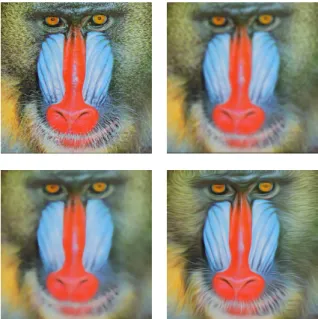
Figure 3.1: Diffusion of a 2D image. (a) original image, (b) linear isotropic diffusion i.e. Gaussian blurring ([15], [56]), (c) nonlinear isotropic diffusion (Perona-Malik [32]), (d) coherence enhancing anisotropic diffusion (using joint color channels in structure tensor) ([53]).

Different processes can be formulated as follows (Figure 3.1): • Linear isotropic diffusion ([15], [56]):

∂tu= div(1∗ ∇u) = ∆u, (3.2)

• Nonlinear isotropic diffusion ([32]):

∂tu= div(g(|∇u|2)∇u), (3.3)

• Nonlinear anisotropic diffusion ([52]):

∂tu= div(D(Jρ(∇uσ))∇u). (3.4)

Following sections will tangle each of them. Finite difference derivative approxi-mations and boundary conditions are explained in Appendix A.1 and A.2.

(42)

Diffusion 30

Linear Isotropic Diffusion Linear diffusion process can be expressed as: ∂tu= ∆u,

u(x,0) = f(x), (3.5)

and is equivalent to Gaussian convolution. It has the unique solution: u(x, t) = ( f(x) (t= 0) (K√ 2t∗f)(x) (t >0) , (3.6)

whereKσis a Gaussian with standard deviationσ: Kσ(x) := 1 2πσ2 exp −|x| 2 2σ2 . (3.7)

The unique solution depends continuously on the initial imagef(well-posedness). The evolving image satisfies the minimum-maximum principle:

inf

R2

f ≤u(x, t)≤sup

R2

f ∀x,∀t >0. (3.8) Other theoretical results include average grey level invariance, Lyapunov se-quences (i.e. transformation is simplifying, information-reducing) and conver-gence to a constant steady state. Mathematical formulation leading to a discrete explicit scheme is given in Appendix A.3.

Nonlinear Isotropic Diffusion Nonlinear isotropic diffusion process can be written as:

∂tu= div(g(|∇u|2)∇u), (3.9)

where g(|∇u|2₎ _{is a diffusivity function governing the nature of the diffusion.}

Contrast parameter λthat separates forward and backward diffusion needs to be set. The function is formed so that the smoothing (forward diffusion) happens for

(43)

Diffusion 31 Some usual diffusivities are:

Perona-Malik diffusivity: g(s2) = 1 1 + s_λ22 , (3.10) Charbonnier diffusivity: g(s2) = _q 1 1 + s2 λ2 , (3.11)

Exponential diffusivity: g(s2_{) = exp}

₋

s2

2λ2

. (3.12)

Properties of function g are g > 0, g ∈ C∞, g(0) = 1, g decreasing on[0,∞),

lim

s2_→∞g(s

2_{) = 0}_{. Mathematical formulation leading to a discrete explicit scheme}

is given in Appendix A.5.

Nonlinear Anisotropic Diffusion Nonlinear anisotropic diffusion process can be written as: ∂tu= div (D(∇u)∇u) = div v1,x v2,x v1,y v2,y ! λ1 0 0 λ2 ! v1,x v1,y v2,x v2,y ! ∇u ! , (3.13)

where v1, v2 are eigenvectors such that v1k∇u, v2⊥∇u and λ1, λ2 eigenvalues

chosen such thatλ2 = 1denotes full diffusion along the edge, andλ1 =g(|∇u|2)

adjustable diffusion across the edge so forming anedge enhancing diffusion. For applications that require a more general structure direction description, the matrix∇u∇uT _{can be used instead of}_∇_u:

∂tu= div D(K∗ ∇u∇uT)∇u = div D K∗ uxux uxuy uxuy uyuy !! ∇u ! = div v1,x v2,x v1,y v2,y ! λ1 0 0 λ2 ! v1,x v1,y v2,x v2,y ! ∇u ! , (3.14)

(44)

Variational Methods 32 such that the smoothing increases with structure coherence i.e.:

λ1 = α, (3.15) λ2 = ( α µ1 =µ2 α+ (1−α) exp −C (µ1−µ2)2 else , (3.16)

where α > 0 is a small value, µ1, µ2 eigenvalues of the structure tensor

K ∗ ∇u∇uT _and _C _{contrast parameter. Such} _{coherence enhancing diffusion} has a better sense of “overall direction” since, due to the structure tensor, the can-cellation of gradients with opposite orientations in not an issue. Mathematical formulation leading to a discrete explicit scheme is given in Appendix A.7.

3.3 Variational Methods

Prior to introduction of vortex area preserving variational methods in Section 3.4.2, variational processes will be presented in this section.

Minimizing an energy functional of the form: Ef(u) = Z Ω (u−f)2 +αΨ |∇u|2 dx, (3.17)

is an elegant way of describing a minimization model and its constraints. The first term, known as data or similarity term is rewarding the similarity to the original imagef, while the second term, know as smoothness term, regulariser or penaliser, penalises deviations from smoothness.

If energy Ef is minimized by functionv, then v satisfiesEuler-Lagrange

equa-tions. A minimizer of the 2D functional: E(u) =

Z

F(x, y, u, ux, uy)dxdy (3.18) necessarily satisfies the Euler-Lagrange equation:

(45)

Variational Methods 33 By using the notation:

F =(u−f)2+αΨ |∇u|2 , Fu = 2(u−f), Fux = 2αuxΨ 0 _|∇ u|2 , Fuy = 2αuyΨ 0 _|∇ u|2 , (3.20)

the following equation is obtained:

0 = (u−f)−α∂x Ψ0 |∇u|2 ux −α∂y Ψ0 |∇u|2 uy giving 0 = div Ψ0(|∇u|2₎_∇_u −u−f α . (3.21)

A choice of how to discretize has to be made.

Discretizing the Euler-Lagrange equations If Euler-Lagrange equations are discretized a non-linear system of equations is obtained. Note that the same sys-tem is obtained if discrete energy functional and its minimizing condition (vanish-ing gradient) is considered directly, without us(vanish-ing the Euler-Lagrange equations (approach used in graphical models):

E(u) = N X i=1 (ui−fi)2 +α N−1 X i=1 Ψ (ui+1−ui)2 h2 , (3.22) ∂E ∂ui = 0, for i= 1, . . . , N , (3.23) where f = (f1, . . . , fN)T is the signal to be restored, u = (u1, . . . , uN)T mini-mizer ofE(u). The system is then solved by using some root finding algorithm.

Euler-Lagrange equations as Parabolic PDEs Another option for discretiza-tion is formulating and solving the Euler-Lagrange equadiscretiza-tion (3.21) as a steady state of a parabolic partial differential equation i.e. forming a diffusion-reaction system: ∂u ∂t = div Ψ 0 (|∇u|2₎_∇_u − u−f α . (3.24)

(46)

Vortex Preserving Diffusion and Variational Processes 34 Such diffusion-reaction system can then be solved in a similar fashion as a diffu-sion process. Mathematical formulation leading to a discrete explicit scheme is given in Appendix A.8.

3.4 Vortex Preserving Diffusion and Variational

Processes

Diffusion based vortex preserving processes are designed in this section. The goal is a vector field in which vortex cores are preserved and rest of the flow dampened. The destruction of other types of features is desired, however, no new features should be created.

Methods for smoothing the vector field that pay attention to the topology of the field have been designed before. Papers like [3] rely on complex combinato-rial topology to process the vector field ([36]). In [27], user is expected to choose the features to be preserved. Here, an automatic method is designed in which the emphasis is on vortex preserving.

Figure 3.2 shows the color coding used for depicting the flow magnitude. Ar-row plots are also used to obtain a better insight into the flow behavior.

(a) (b) (c) (d) (e)

Figure 3.2: (a) color coding used to depict the vector direction (color) and magnitude (saturation), (b) color coded magnitude of a analytical test flow field with two centers and two saddles, (c) arrow plot of the vector field from (b) (also in Figure 2.3 (d)). (d) color coded magnitude of a flow field saved from a paused 2D real-time simulation, (e) arrow plot of the vector field from (d).

(47)

Vortex Preserving Diffusion and Variational Processes 35 Section 3.4.1 presents different diffusion methods for preserving the swirling features. Nonlinear isotropic diffusion is used with different diffusivities designed to preserve vortices. Diffusivities are based on using the discriminant d of the characteristic polynomial of the Jacobian matrix in each point of the flow.

(a) (b) (c) (d)

Figure 3.3: Critical points detected in the flow fields from Figure 3.2. (a), (c) Critical points detected as intersection of curves where flow components change sign. (b), (d) Vortex cores i.e. critical points where d < 0i.e. swirling critical points, foci or centers (denoted as red diamonds).

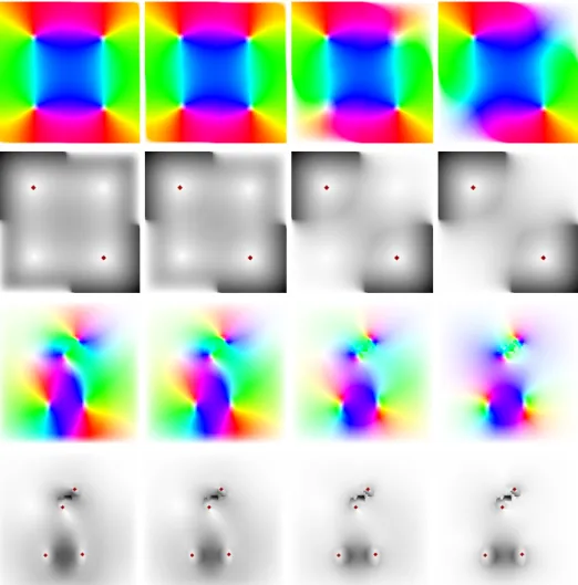
In 2D stationary vector fields, the vortex/swirling critical point exists if the eigen-values of the Jacobian matrix are two conjugated complex eigen-values i.e. if the dis-criminant of the quadratic equation:

λ1,2 = trJ ±p tr2_J₋₄_|_J_| 2 , (3.25) where J = ux uy vx vy !

, is less than zero i.e. d = (ux −vy)2 + 4uyvx

< 0. Figure 3.3 shows critical points detected in 2D vector fields from Figure 3.2. The critical points are detected by locating the intersections of the curves where the components of the vector field change direction. In (b) and (d) only the points whered <0i.e. vortices are shown. Figure 3.4 shows the areas in the test vector fields where the quantityd <0.

Binary diffusivity, binary diffusivity with additional edge blurring and con-tinuous diffusivities are presented. Swirling area indicated by the negative dis-criminant ddoes not guarantee that there is a critical point within it. To always obtain only areas around vortices, binary diffusivities based on vortex (core or re-gion) detection are also presented. Diffusion-reaction processes are presented in Section 3.4.2. Resulting flow fields are smoothed, but have emphasized/preserved

(48)

Vortex Preserving Diffusion and Variational Processes 36

(a) (b) (c) (d)

Figure 3.4:(a), (c) Areas in test vector fields where discriminantd <0denoted red, (b), (d) Swirling areas together with swirling critical points denoted blue.

swirling features i.e. vortices.

3.4.1 Vortex Preserving Diffusion

A diffusion processes are designed with diffusivity function that avoids swirling features or vortices. Nonlinear isotropic diffusion process is taken:

∂tu= div(g(|∇u|2)∇u), (3.26)

with functiong being a diffusivity function governing the nature of the diffusion (see Section 3.2, Appendix A.5).

Wanted properties for the functiong are that it is positiveg > 0and smooth g ∈ C∞[0,∞). These properties ensure that the diffusion process is well-posed and regular, the average gray level is preserved, the minimum-maximum principle respected, that the process is simplifying and information-reducing, and that for t → ∞the image converges to the average gray level (average flow magnitude).

Selecting a diffusivity function which equals zero for certain cases, results in a process that does not converge to the average steady state. Flow areas for which g = 0 do not get diffused, so for t → ∞the process converges to the average magnitude outside these areas, while the flow inside stays unchanged. A small variance of the flow magnitude within the blurred area is a good stopping criteria for all presented methods.

Binary Diffusivity Diffusivityg is set to strong in a non-swirling area (where d ≥ 0) and set to weak where there are swirling features (d < 0). Following

(49)

Vortex Preserving Diffusion and Variational Processes 37 diffusivity is constructed: g(s2) = ( 0, d <0 1, d≥0 . (3.27)

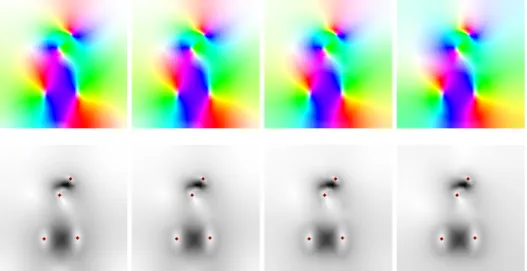
Note that forg = 1nonlinear isotropic diffusion equals the linear isotropic diffu-sion i.e. Gaussian blurring. Figure 3.5 shows the diffudiffu-sion process on the two test vector fields for different number of iterations.

Figure 3.5: Nonlinear isotropic diffusion process with diffusivity (3.27) on an analytical test flow field (upper two rows) and simulated test flow field (lower two rows) for iteration number: 500,1000,5000,50000(left to right). Upper, third row: color coded magnitude of the flow. Second, lower row: gray scale flow magnitude with vortex cores. Red critical points are the points originally present in the vector field. Orange critical points are newly created.

(50)

Vortex Preserving Diffusion and Variational Processes 38 Figure 3.6 shows the arrow plots of the processed flow fields for high iteration number (50000).

(a) (b) (c) (d)

Figure 3.6: (a), (c) arrow plots of the two test vector fields, (b), (d) arrow plots of the diffused vector fields from Figure 3.5 right (50000iterations).

Swirling structures are preserved and the rest of the field blurred, however, new critical points are introduced at the borders of the swirling and non-swirling ares (orange points in Figure 3.5).

Additional Blurring of the Swirling Structure Edges Newly introduced critical points need to be removed. They appear at the places where discriminant dchanges sign. Figure 3.7 shows the areas whered >−, whereis small. The threshold chooses the area whered >0plus edge of thed <0area (Figure 3.4).

(a) (b) (c) (d)

Figure 3.7: Areas where discriminant (a), (c)d >−0.0001and (b), (d)d >−0.01. The area whered >0is chosen plus the edge of thed <0area (Figure 3.4).

(51)

Vortex Preserving Diffusion and Variational Processes 39 Additional Gaussian blurring of the area with d > −0.01is performed after the diffusion process with the diffusivity (3.27). This removes the created invalid critical points. Figure 3.8 shows such process.

Figure 3.8: Nonlinear isotropic diffusion process with diffusivity (3.27) followed by blurring for iteration number: 500,1000,5000,50000 (left to right). Upper, third row: color coded magnitude of the flow. Second, lower row: gray scale flow magnitude with vortex cores.

Figure 3.9 shows arrow plots of the processed flow fields for high iteration num-ber. Swirling features are preserved and no new features are introduced. Sharp boundaries between the swirling and non swirling areas are blurred.

(52)

(a) (b) (c)

(d) (e) (f)

Figure 3.9: (a), (d) arrow plots of the two test vector fields, (b), (e) arrow plots of the diffused vector fields from Figure 3.5 right (50000iterations), (c), (f) arrow plots of the diffused and additionally blurred fields from Figure 3.8 right (50000iterations).

Continuous Diffusivity Previous process first blurs the area whered > 0, and then, because the sharp blurring border introduces additional critical points, the area whered > −0.01is blurred. This removes the introduced artifacts. Alterna-tive solution is designing a diffusivity without sudden jumps. Following diffusiv-ity is now considered:

g(s2) =      0, d <0 d, d∈[0,1] 1, else , (3.28) where discriminant d = (ux −vy)2 + 4uyvx

. This results in an graduate in-crease of blurring amount, from no blurring within the swirling area to full blur-ring (g = 1) away form the swirling area. During the diffusion process, additional blurring iteration is made within the non-swirling area to further blur it out. Fig-ure 3.10 shows the value of the discriminant of the two test vector fields mapped to grayscale. Sudden jumps in values are not excluded. Figure 3.11 shows the diffusion process. Figure 3.12 compares the arrow plots of this and two previous approaches.

(53)

(a) (b) (c)

Figure 3.10:Value of the discriminantdof the two test vector fields mapped to grayscale. Negative values start from white, positive end with black. (a) analytical example, (b) frame from the real-time simulation test data, (c) middle image with adjusted contrast and brightness.

Figure 3.11: Nonlinear isotropic diffusion process with diffusivity (3.28) for iteration number: 500,1000,5000,50000(left to right). Upper, third row: color coded magnitude of the flow. Second, lower row: gray scale flow magnitude with vortex cores.

(54)

(a) (b) (c) (d)

(e) (f) (g) (h)

Figure 3.12: (a), (e) arrow plots of the two test vector fields, (b), (f) arrow plots of the diffused vector fields (3.27) from Figure 3.5 right (50000iterations), (c), (g) arrow plots of the diffused and additionally blurred fields from Figure 3.8 right (50000 iterations). (d), (f) arrow plots of the diffused vector fields (3.28) from Figure 3.11, right (50000 iterations).

Shown processes output the vector fields with emphasized swirling features. No new swirling features are introduced, however, it is not always guaranteed that all other features are destroyed. Figure 3.13 shows the resulting vector fields with all critical points denoted. The diffusion with diffusivity (3.27) destroys all other features, but also introduces new critical points. Approach with additional blurring after the diffusion and the diffusion with diffusivity (3.28) do not guarantee the destruction of the non-swirling critical points. They do, however, emphasize the swirling features and produce relatively smooth vector fields without introducing new swirling features.

(55)

Figure 3.13: All critical points within the two processed vector fields with50000 itera-tions. Swirling critical points are denoted red, non-swirling critical points green. Upper row: analytical flow field, lower row: frame from the real-time simulation. Left column: initial vector fields, Second column: diffusion with diffusivity (3.27), Third column: dif-fused with diffusivity (3.27) plus additional blurring, Right column: diffusion with diffu-sivity (3.28).

Binary Diffusivity Based on Vortex Detection Presented diffusion approaches are steered by the discriminant dof the characteristic polynomial of the Jacobian matrix. Areas where d < 0do not always nicely indicate an area around vortex cores. There is also no guarantee that there is a swirling critical point present within the swirling area. This results in seemingly random patches of flow which are not smoothed. Figure 3.14 shows such an example. It represents another vec-tor field saved from a 2D real-time simulation processed with nonlinear isotropic diffusion with diffusivity (3.27). Although the swirling areas are preserved, it is not the result one would necessarily desire as a field with emphasized vortices.

An alternative approach is to detect vortex cores, and to not blur the vector field in areas around them. This process could also be considered a nonlinear isotropic diffusion process with binary diffusivity steered by the location of vortex cores i.e. with diffusivity:

g(s2) = (

0, areas around vortex cores

(56)

Vortex Preserving Diffusion and Variational Processes 44 Figure 3.15 shows the result of such process for two different area sizes. Resulting flow fields have preserved swirling areas around the vortex cores. There are no newly created critical points.

Figure 3.14:Nonlinear isotropic diffusion process with diffusivity (3.27) on a simulated flow field. Swirling areas without swirling critical points remain unblurred.

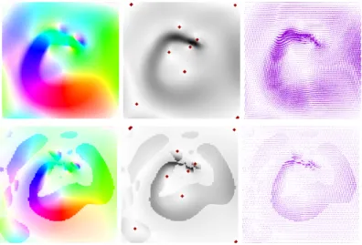
Figure 3.15:Nonlinear isotropic diffusion process with diffusivity (3.29) on a simulated flow field (same as in figure 3.14) for 50000 iterations. Upper row: smaller area sur-rounding the vortex cores. Lower row: bigger area sursur-rounding the vortex cores. For better visibility, right column shows arrow plots of the vector field with increased magni-tude. First column: color coded magnitude of the vector field. Second column: magnitude of the vector field together with swirling critical points (red) and area surrounding them (blue).

(57)

Vortex Preserving Diffusion and Variational Processes 45 Considering vortex region detection gives another option for defining the vor-tex areas to be preserved. Q criterion for vorvor-tex region detection is taken as a vortex indicator ([14], Section 4.2.1). Areas where the vorticity tensorA= J−₂JT

dominates the rate of strain tensorS = J+₂JT are considered (J Jacobian matrix). This is achieved by looking at the ratio of the Euclidean norm of the two matrices. The diffusivity is then defined as:

g(s2) = (

0, areas around points where |_|A_S_||22 >1

1, else . (3.30)

Figure 3.16 shows the test vector fields processed with diffusion (3.30). In practice an area around|A|2 _>_|_S_|2₊_{with small}_{is chosen to get the preserved vortex}

area (Figure 3.16, upper row).

Figure 3.16: Nonlinear isotropic diffusion process with diffusivity (3.30) on test flow fields for50000iterations. Upper row: left: area where|A|2 _>_|_S_|2_{, middle: area where}

|A|2_>_|_S_|2₊_{, right: area surrounding}_|_A_|2_>_|_S_|2₊_{. Second, third row: diffusion on}

test flow fields. Left: original magnitude, middle: magnitude of the diffused vector field, right: magnitude of the vector field together with swirling critical points (red) and area surrounding them (blue). Lower row: arrow plots of the shown vector fields.