The Application of Single porosity Model to Predict the Performance of the Low Permeability Naturally Fractured Formations

(1)

Graduate Theses, Dissertations, and Problem Reports

2012

The Application of Single porosity Model to Predict the

Performance of the Low Permeability Naturally Fractured

Formations

Martial Hermann Tchuindjang Yatchou

West Virginia University

Follow this and additional works at: https://researchrepository.wvu.edu/etd Recommended Citation

Recommended Citation

Tchuindjang Yatchou, Martial Hermann, "The Application of Single porosity Model to Predict the Performance of the Low Permeability Naturally Fractured Formations" (2012). Graduate Theses, Dissertations, and Problem Reports. 319.

https://researchrepository.wvu.edu/etd/319

This Thesis is protected by copyright and/or related rights. It has been brought to you by the The Research Repository @ WVU with permission from the rights-holder(s). You are free to use this Thesis in any way that is permitted by the copyright and related rights legislation that applies to your use. For other uses you must obtain permission from the rights-holder(s) directly, unless additional rights are indicated by a Creative Commons license in the record and/ or on the work itself. This Thesis has been accepted for inclusion in WVU Graduate Theses, Dissertations, and Problem Reports collection by an authorized administrator of The Research Repository @ WVU. For more information, please contact researchrepository@mail.wvu.edu.

(2)

The Application of Single porosity Model to Predict the Performance of the Low Permeability Naturally Fractured Formations

Martial Hermann Tchuindjang Yatchou

Thesis submitted to the

Benjamin M. Statler College of Engineering and Mineral Resources at West Virginia University

in partial fulfillment of the requirements for the degree of

Master of Science in

Petroleum and Natural Gas Engineering

Kashy Aminian, Ph. D. Committee Chair Samuel Ameri, M.S.

Ilkin Bilgesu, Ph. D.

Department of Petroleum and Natural Gas Engineering

Morgantown, West Virginia 2012

Keywords: Single Porosity, Dual Porosity, Production Performance Prediction, Low Permeability, Naturally Fractured Formations

(3)

ABSTRACT

The Application of Single porosity Model to Predict the Performance of the Low Permeability Naturally Fractured Formations

Martial Hermann Tchuindjang Yatchou

Natural gas extraction from shale is currently an expensive endeavor due to the tight reservoir rock with nano-darcy permeability. New technology in the form of horizontal drilling and hydraulic fracturing (fracturing through the use of high pressure liquids) has overcome the flow capacity problem of shale to achieve economic production. The low permeability shale formations, such Marcellus Shale, contain a natural fracture system with extremely low permeability. The characteristics of the natural fracture system are non-existent; therefore the application of single porosity model to predict the production performance of the shale formations can reduce the need for detail fracture system characteristics.

The objective of this research is to conduct a reservoir modeling study to investigate the applicability of the single porosity model to predict the performance of hydraulically fractured shale reservoirs. A commercial reservoir simulator (ECLIPSE) was employed to generate different production profiles for a hydraulically fractured shale reservoir using the dual porosity model. The production profiles were then history-matched with a single porosity model. The history matching results were then utilized to determine the single porosity model parameters that approximate the dual porosity behavior. The results suggested that the entire production history cannot be matched with a single set of parameters for single porosity model. The time over which the production can be approximated by single porosity model was also identified. The results are used to investigate the impact of hydraulic fractures at the early production period.

(4)

iii

ACKNOWLEDGEMENTS

This project would not have been possible without the support of many people.

I am extremely thankful to my supervisor Dr. Kashy Aminian for his commitment and his infinite help throughout my research.

Also thanks to my committee members Professor Samuel Ameri Chair of Petroleum & Natural Gas Engineering Department and Dr. Ilkin Bilgesu for their noble guidance, support with full encouragement and enthusiasm. Furthermore, I would like to thanks the rest of the Petroleum and Natural Gas Engineering Department faculty and staff for their help and friendly ambience.

Thanks to the Benjamin M. StatlerCollege of Engineering and Mineral Resources for providing me with an exceptional engineering background.

Last but not the least I would also like to dedicate sincerely my entire success to my family members and friends for encouraging and supporting me whenever I needed them.

(5)

iv

LIST OF FIGURES

FIGURE 1: UNCONVENTIONAL GAS PROJECTION IN THE U.S ... 3

FIGURE 2: RESOURCE TRIANGLE FOR UNCONVENTIONAL GAS ... 4

FIGURE 3: FUTURE PROJECTIONS OF NATURAL GAS PRODUCTION ... 5

FIGURE 4: UNITED STATES SHALE GAS PLAYS ... 5

FIGURE 5: BASIC MULTILATERAL CONFIGURATIONS ... 9

FIGURE 6: REPRESENTATION OF SHALE GAS EXTRACTION TECHNIQUE ... 11

FIGURE 7: SCHEMATIC OF DUAL POROSITY MODEL USING THE WARREN AND ROOTS MODEL ... 12

FIGURE 8: FLUID DISPLACEMENT INSIDE OF THE RESERVOIR ... 14

FIGURE 9: 4000 FT X 2000 FT DRAINAGE AREA WITH 3000 FT LATERAL AT THE CENTER ... 18

FIGURE 10: 4000 FT X 1000 FT DRAINAGE AREA WITH 3000 FT LATERAL AT THE CENTER ... 19

FIGURE 11: FLOWCHART OF THE ANALYSIS PROCESS ... 20

FIGURE 12: IMPACT OF HYDRAULIC FRACTURES ON PERMEABILITY (DRAINAGE AREA: 4000 FT X 1000 FT) ... 24 FIGURE 13: IMPACT OF HYDRAULIC FRACTURES ON POROSITY (DRAINAGE AREA: 4000 FT X 1000 FT) ... 24 FIGURE 14: IMPACT OF HYDRAULIC FRACTURES ON PERMEABILITY (DRAINAGE AREA: 4000 FT X 2000 FT) ... 26 FIGURE 15: IMPACT OF HYDRAULIC FRACTURES ON POROSITY (DRAINAGE AREA: 4000 FT X 2000 FT) ... 26 FIGURE 16: DETAILED CURVE CASE # 1 EARLY PERIOD ... 28

FIGURE 17: DETAILED CURVE CASE # 1 LATE PERIOD ... 29

(7)

vi

LIST OF TABLES

TABLE 1: COMPARISON OF DATA FOR THE SHALE IN U.S ... 7

TABLE 2: VITRINITE REFLECTANCE FOR SHALE GAS RESERVOIRS ... 7

TABLE 3: PARAMETERS AND VALUES USED FOR THE BASE MODEL ... 17

TABLE 4: VARIOUS RESERVOIR DRAINAGE AREA CONFIGURATIONS ... 18

TABLE 5: EVALUATED CASE STUDIES USED ... 19

TABLE 6: SUMMARY OF CASE # 1 AND CASE # 2 (DRAINAGE 4000 X 1000 FT) AT 10 YEARS ... 21

TABLE 7: SUMMARY OF CASE # 3 AND CASE # 4 (DRAINAGE 4000 X 1000 FT) AT 10 YEARS ... 22

TABLE 8: SUMMARY OF CASE # 5 (DRAINAGE 4000 X 1000 FT) AT 10 YEARS ... 23 TABLE 9: SUMMARY OF CASE # 1 AND CASE # 2 (DRAINAGE AREA 4000 FT X 2000 FT) ... 25 TABLE 10: SUMMARY OF CASE # 3 AND CASE # 4 (DRAINAGE 4000 X 2000 FT) AT 10 YEARS ... 25 TABLE 11: SUMMARY OF CASE # 5 (DRAINAGE 4000 X 2000 FT) AT 10 YEARS ... 25 TABLE 12: SUMMARY OF CASE # 1 (DRAINAGE 4000 x 1000 FT) BEFORE 10 YEARS....………27

TABLE 13 SUMMARY OF CASE # 1 (DRAINAGE 4000 X 2000 FT) BEFORE 10 YEARS………27

TABLE 14: SUMMARY OF CASE # 1 (DRAINAGE 4000 X 1000 FT) AFTER 10 YEARS………..30

(8)

1

CHAPTER I INTRODUCTION

In the United States, the gas production has increased significantly due to the discovery of the unconventional (low permeability) gas reservoirs. The resources associated with unconventional gas include low-permeability shale oil and gas reservoirs, and tight gas formations. Unconventional resources, characterized by their low gas recovery rate are seen as challenging. For example, gas recovery factor for these unconventional resources is estimated at 10-30% of GIP, much lower from conventional gas reservoirs (SPE 142884). Shale reservoirs have low permeability (less than 0.01 mD) and hence cannot be extracted via conventional methods. Technology such as horizontal drilling coupled with hydraulic fracturing to force natural gas from these low permeability geologic formations has greatly expanded the ability of the producers to profitably recover natural gas.

Natural fractures are important in the economical production of low permeability formations. A naturally fractured reservoir (NFR) can be defined as a reservoir that contains fractures (planar discontinuities) created by natural processes like volume shrinkage, distributed as a consistent connected network throughout the reservoir (Ordonez et al., 2001).

The effective modeling technique of naturally fractured reservoirs (NFR) has been through a dual porosity approach, where the fracture and matrix systems are separated into two different continuums, each with its own set of properties. Introduced in the late 1940s (Clark 1949;

Howardand Fast, 1970), hydraulic fracturing has been used commonly to stimulate well production in gas industry in the last few decades. Horizontal wells with multiple fracture treatments have proven to be an effective method for producing economically from shale.

(9)

2

For this study, two main approaches including single porosity (SP) and Dual porosity (DP) have been used. The history matching results were then utilized to determine the single porosity model parameters that approximate the dual porosity behavior. To achieve this goal, several cases were modeled using different drainage areas to evaluate the production performance of fractured horizontal wells.

(10)

3

CHAPTER II LITERATURE REVIEW

II. 1 Unconventional gas reservoirs

Unconventional gas is poised to dominate U.S gas production in coming decades. In the USA, the production from unconventional gas resources has increased since late 2000 and now approximates 87 Tcf/yr, as shown in Figure1.

Figure1: Unconventional gas projection in the U.S (EIA, 2008)

As illustrated in Figure 2, conventional reservoirs, are limited in volume, high in permeability and easy to develop, unconventional reservoirs on the other hand are expansive in volume, very low in permeability (micro-Darcy range or less) but difficult to develop. They are not feasible to be produced at economic flow rates, therefore require special gas extraction techniques.

(11)

4

Figure 2: Resource triangle for unconventional gas (Holditch, 2006)

The commonly types of unconventional gas reservoirs are tight gas, coal bed methane and shale gas. They currently accounts for 58 percent of the total U.S production.

II. 2 Shale Gas

Shale gas production is expected to be the driving force behind increased natural gas production, increasing from 5.0 trillion cubic feet in 2010 to 13.6 trillion cubic feet in 2035, accounting for nearly half of all domestic natural gas production as illustrated in Figure 3. (Image: U.S EIA 2012). With technically recoverable U.S. shale gas resources now estimated at 1,744 trillion cubic feet (Tcf) including 211 Tcf of proven reserves. Shale gas resources constitute 34 percent of the domestic natural gas resource (AEO, 2011) and 44 percent of lower 48 onshore resources Figure 4 is a visualization of lower 48 states shale plays.

(12)

5

Figure 3: Future projections of natural gas production (trillion cubic feet)

(13)

6

Shale is a sedimentary rock formation which contains clay, quartz and other minerals. In terms of chemical composition, gas produced from the Shale is typically dry gas composed primarily of methane, but water can also be produced from shale gas formations. The Antrim shale and New Albany shale are the typical cases as shown in Table 1 (J. Daniel Arthur et al. 2008).

Shale reservoirs have low permeability (less than 0.01 mD). Aside from permeability, their key properties, when considering gas potential, are total organic content (TOC) and thermal maturity. TOC is the total amount of organic material (kerogen) present in the rock, expressed as a percentage by weight.

∅

Where

∅

= Kerogen volume (volume/volume)

=

Kerogen density (g/ cubic centimeter)

=

Bulk density (g/ cubic centimeter) K = Kerogen conversion factor

Generally, the higher the TOC, the better is the potential for hydrocarbon generation. Table 1 summarizes the TOC of different type of shale formations. The thermal maturity of the rock is a measure of the degree to which organic matter contained in the rock has been heated over time, and potentially converted into liquid and/or gaseous hydrocarbons. Thermal maturity is measured using vitrinite reflectance (Ro) which is measured by the core analysis. Table 2 summarizes the vitrinite reflectance for shale reservoirs.

(14)

7

Table 1: Comparison of data for the shale in U.S (J. Daniel Arthur et al., All Consulting 2008)

(15)

8

The total amount of gas in place within the shale will determine how economical the shale play is. The gas is a combination of 1) free gas in the pores (Gf), 2) absorbed gas on the organics

(Ga), 3) dissolved gas into the liquid hydrocarbon (GSO) and 4) dissolved gas into the formation

water (GSW).

Hence, the total gas in place (Gst) is defined as: Gst = Gf + Ga + GSO+ GSW (Eq. 1)

Where Gf = 32.0368 ∅

(Eq. 2) Ga =

(Eq. 3) GSO = . . ∅

(Eq. 4) GSW = . . ∅

(Eq. 5)

However (Eq. 4) and (Eq. 5) are not applied. These are usually ignored or lumped in with adsorbed gas.

Given the low permeability of these shale reservoirs, the gas must be developed via special techniques including Horizontal drilling and fracture stimulation both have been crucial in the development of the shale gas industry.

(16)

9

II. 3 Technique of gas extraction II. 3. 1 Drilling Methods

Horizontal drilling is a technique that allows the wellbore to come into contact with significantly larger areas of hydrocarbon bearing rock than in a vertical well Figure5. As a result of this increased contact, production rates and recovery factors can be increased. As the technology for horizontal drilling and hydraulic fracturing has improved, the use of horizontal drilling has increased significantly. Much more sophisticated drilling technologies such as multilateral drilling have done theirs appearances these recent years. According to the TAML group (Technical Advancements of Multi-Laterals), multilateral wells are wells with several laterals either vertical or any inclination up to or greater than horizontal. The following schematic represents the multilateral configurations.

(17)

10

II. 3. 2 Hydraulic fracturing

The most common method of well stimulation is hydraulic fracturing as illustrated in figure 5. Introduced in the late 1940s (Clark 1949; Howardand Fast, 1970), Hydraulic fracturing is a formation stimulation practice used to create additional permeability in a producing formation. By creating additional permeability, hydraulic fracturing facilitates the migration of fluids to the wellbore for purposes of production (Veatch, Ralph W. Jr. et al.). According to Ozkan et al (2009), hydraulic fracturing objectives are to increase fracture density and decrease fractures spacing, therefore can both increase production rates and increase the total amount of gas that can be recovered from a given volume of shale. The process of hydraulic fracturing involves the pumping of thousands of barrels of mixed sand and water into the target shale zone. Figure 6 shows a brief view of the technique. Fluids pumped into the shale creates fractures or openings through which the sand flows, at the same time acts to pro open the fractures that have been created (J. Daniel Arthur et al. 2008)

The important factor in hydraulic fracturing is the Dimensionless fracture conductivity (CrD). The conductivity is the product of the thickness of zone times its permeability. According to John Lee (2003), the fracture conductivity is given by the following formula:

C

rD

=

Where

C

rD

>

100, the fracture behavior is considered infinite conductivity.

C

rD < 100, the fracture behavior is considered finite conductivity.

(18)

11

(19)

12

II. 4 Dual Porosity Model

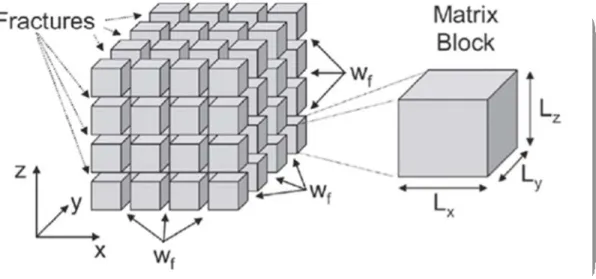
The shale formation is typically a naturally fractured system. A qualitative description of a naturally fractured reservoir was given as early as 1953 by Pirson as reservoir with two porous structures-matrix (porous rock) and fracture. The most prevalent approach in the simulation of naturally fractured formation is a dual porosity formulation in which the rock matrix is defined as a series of discontinuous matrix blocks within a continuous fracture system.

The foundations of the dual porosity model were constructed by Barenblatt et al. (1960) and Warren and Root (1963). The assumptions for, their dual porosity model was as following:

 Uniform continuity of fracture network parallel to the principal axes of permeability.  The matrix blocks and the fracture network are identical in shape (rectangular

parallelepipeds) and located in the same space.

 There is an isotropic and homogeneity within the matrix blocks. The Warren and Root (1963) model is illustrated in Figure 7.

(20)

13

The mathematical approach that model is a 2D fracture domain and slightly compressible fluids (Warren and Root, 1963), defined as:

∅

(Eq. 6)

According to Warren and Root (1963), The Darcy’s flow is applicable if the pseudo steady state exists in the matrix system, therefore the following equation must be satisfied.

∅

(Eq. 7)

Where

(Eq.6) is the equation governing fluid flow in the fracture system (Eq. 7) is the equation governing the matrix system

(Eq. 8)

The Factor defines the isotropic of matrix blocks and also controls fluid exchange between fractures and matrix

There are two types of porosity existing in naturally fractured reservoirs: fracture porosity and matrix porosity. The fluid flows from a porous matrix (low permeability) usually representing the reservoir storage volume for free gas and adsorbed gas into a fractured system (high permeability) then to the wellbore. In the case of injection, the injected fluid displaces the fluid inside the matrix. (John D. Hudson, 2011)

(21)

14

Figure 8: Fluid displacement inside of the reservoir. The small arrows represent flow from the porous matrix to the fracture network and the large arrows represent flow inside the matrix.

(22)

15

CHAPTER III

OBJECTIVES & METHODOLOGY

III. 1 Objective

The goal of this research was toinvestigate the applicability of the single porosity model. To achieve this goal, the following tasks were performed and are described here:

 Develop a reservoir model using a commercial reservoir simulator (ECLIPSE)  Establish of production profiles for dual and single porosity models.

 History-match of production profiles obtained from dual porosity model with a single porosity model to determine the single porosity model parameters that approximate the dual porosity behavior.

 Identify the intervals over which the production can be approximated by different set of single porosity model parameters.

III. 2. Methodology

III.2.1. Reservoir Models and Assumptions

Two reservoir base models were developed using the software ECLIPSE by Schlumberger to generate different production profiles for hydraulically fractured formations. Figure 8 & 9 illustrate the configuration models. A dual porosity (DP) model and single porosity (SP) model were considered with absorbed gas accounting for the dual porosity. One layer was used for both models (DP & SP) to run the simulation. A horizontal well is centered in the middle of the reservoir using no fracture, 1, 3, 4, 5, 6, 7 and 11 fractures. The mathematical model constructed for this study is a 3D Cartesian with regular grids. Using the single porosity model, the need of detailed parameters was reduce, just one set of data was used and it was easy to run; while more assumption modes and too much detailed parameters for the dual porosity model.

(23)

16

III.2.1.2 Model parameters

The parameters used for simulation in this study were based on the published data (Belyadi et Al. 2010), Table 3 summarizes the parameters used to generate the basic model.

(24)

17

(25)

18

III.2.1.3 Model Development

The geometric drainage shape of the reservoir was rectangular. Various reservoir drainage areas were considered and are illustrated in Table 4.

Table 4: Various reservoir drainage areas configuration

The analysis was performed using the completions tool model template in ECLIPSE. The developed reservoirs were producing at constant rate with 40 years length simulation. More than 300 runs were done to better understand the applicability of the single porosity. Marcellus shale characteristics are the main component of this simulation model.

(26)

19

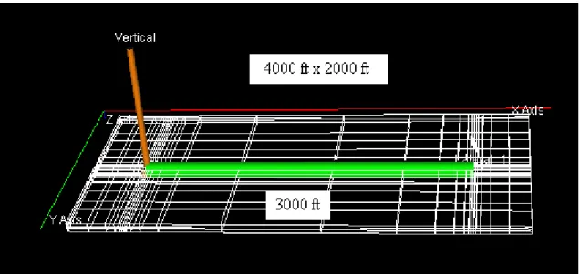
Figure 10: 4000ft x 1000ft Drainage area with 3000 ft lateral at the center

Once the both reservoir models (DP & SP) were developed, the production profiles were then simulated. A history matching was conducted for each evaluated study cases to determine the single porosity model parameters that approximate the dual porosity behavior. By setting up the dual porosity parameters and keeping them constant and by varying just the single parameters, the results were determined.

The values of dual porosity model parameters were either increased or decreased based on different case scenarios. The single porosity parameters were varied until getting the closest value that approximate the dual porosity curve

The coal bed methane template was considered to account for the absorbed gas. Table 5 shown below summarizes the different evaluated study cases conducted in this simulation.

(27)

20

III.2.1.4. The Analysis Process

The set of parameters for single porosity model were obtained using the flowchart in Figure 10 that explains how the entire process was carried out.

(28)

21

CHAPTER IV

RESULTS AND DISCUSSIONS

IV. 1. Results

The main objective of this chapter is to determine a set of the single porosity model parameters that approximate the dual porosity model. The results obtained derive from 5 different case studies (refer to Table 3). Two different drainage areas with same horizontal lateral configuration (4000 ft * 1000 ft, 4000 ft * 2000 ft and 3000 ft lateral) were utilized for each case. However for the second drainage area only for 7, 9 and 11 hydraulic fractures were simulated. All production profiles were generated with a simulation length of 40 years period.

The following are the results for different cases with different drainage areas.

Drainage area: 4000 ft * 1000 ft at 10 years

(29)

22

(30)

23

(31)

24

Figure 12: Impact of Hydraulic Fractures on Permeability

(32)

25

Drainage area: 4000 ft * 2000 ft at 10 years

Table 9: Summary of case # 1 and case # 2

Table 10: Summary of case # 3 and case # 4

(33)

26

Figure14: Impact of Hydraulic Fractures on Permeability

(34)

27

Drainage area: 4000 ft * 1000 ft. Before 10 years

Table 12: Summary of Case # 1

Drainage area: 4000 ft * 2000 ft. Before 10 years

(35)

28

Figure16: detailed curve case # 1. Early period

(36)

29

Figure17: detailed curve case # 1. Late period

(37)

30

Drainage area: 4000 ft * 1000 ft. After 10 years

Table 14: Summary of Case # 1

Drainage area: 4000 ft * 2000 ft. After 10 years

(38)

31

IV. 2. Discussion

All figures listed in appendix A illustrate the impact of hydraulic fractures on single porosity model parameters (porosity and permeability) for all different 5 cases. The fractures are uniformly spaced and have same properties. The first 10 years production is investigated for economic reason because of the production depletion. Figures A, B, C, D, and E in Appendix A compare both dual and single porosity curves. For each case listed with different number of hydraulic fractures from 0 to 11 fractures; the trends are similar.

When we look at the whole 40 years of production especially at 10 years, it is seen that from 0 to 7 hydraulic fractures the entire production cannot be matched just with one set of parameters of single porosity model, while the number of hydraulic fractures increase from 9 to 11 fractures the dual porosity and single porosity curves got a perfect match. That means the production is not longer controlled by the single porosity model but by the hydraulic fractures. Therefore when the number of fractures increase the production becomes significant. Figures A, B, C, D, and E in appendix A illustrate that. Seen that the entire production cannot be matched by a set of parameters, two periods of production have been identified to clearly approximate the production by the different set of parameters.

The first period investigated is the early period (before 10 years). As it is seen, the dual porosity model can only be approximated by a single set of parameters, but the late period is not getting matched. That means after the first 10 years different set of parameters is needed in order to approximate the production as shown in case # 1, Figures Fs. To better clarify the approximation of the production at first period, Case # 1 has been investigated as an example for both different drainage areas accounting for 0, 1, 3, 4, 5, 6, 7, 9 and 11 fractures. Referring to the single set of parameters at 10 years period Table # 6, the porosity value is either increased or decreased until get close enough to the match. For instance, case # 1(Figure 16: 1 fracture) shows that the single porosity model curve clearly matches the dual porosity curve at the early stage.

The second period is the late period (after 10 years). By having a sight on all Figures Gs listed in the in appendix A, the production can be approximated but not at the early period. Therefore, only a different set of parameters of single porosity can only be adjusted to match the dual porosity curve.

(39)

32

Varying different porosities values as it is for the early period, the closest approximation has been achieved. The case # 1 (Figure 17: 1 facture) has still been detailed as example.

All different set of parameters for with their different intervals of time is illustrated in Table # 6 through Table # 15.

Although there are some differences in the production profiles generated by the two models, the results are very similar. An interesting observation made is that increasing the drainage area width from 1000 ft to 2000 ft does not have any particular effect on the single porosity model. All set of parameters for single porosity model on both drainage are similar.

As it has been said in the previous chapter that the model accounts for absorbed gas; based on previous literature reviews, desorption gas was found to have no impact during early production (Belyadi, et al 2010 and 2012).

(40)

33

CHAPTER V CONCLUSIONS

The objective of this research was to investigate the applicability of the single porosity model to predict the performance of hydraulically fractured shale reservoirs. In addition, the intervals over which the production can be approximated by single porosity model was also identified. The results from this work allow drawing the following conclusions:

 The entire production history cannot be matched with a single set of parameters for the single porosity model.

 The single porosity parameters are not impacted by the drainage area.

 As the number of hydraulic fractures increase, the production becomes significant.

Therefore the application of single porosity model to predict the production performance of the shale formations can reduce the need for detail fracture system characteristics.

(41)

34

REFERENCES

Belyadi, A., Aminian, K., Ameri, S. (2012). Production performance of multiply fractured horizontal wells. SPE 153894

Belyadi, A., Aminian, K., Ameri, S. (2010). Performance of the hydraulically Fractured Horizontal Wells in Low Permeability Formation. SPE 139082

F. Medeiros, B. Kurtoglu, E. Ozkan, H. Kazemi,(2007). Analysis of Production Data From Hydraulically Fractured Horizontal Wells in Shale Reservoirs. SPE 110848

G.C. Naik (n.d). Tight Gas Reservoirs – An Unconventional Natural Energy Source for the Future

J. Daniel Arthur; Brian Bohm, P.G; Bobbi Jo Coughlin; Mark Layne. (2008). Evaluating The Environmental Implications of Hydraulic Fracturing in Shale Gas Reservoirs.

John .D, Hudson (2011). Quad porosity model for description of gas transport in shale gas reservoirs. Master of Science. University of Oklahoma.

Haider J. Abdulal., Orkhan, Samandarli., & Robert A, Wattenbarger. (2011). New Type Curves for Shale Gas Wells with Dual Porosity Model. CSUG/ SPE 149367

Pallav Sarma and Khalid Aziz (2006). New transfer functions for simulation of naturally fractured reservoirs with dual porosity models. SPE 90231

Pallav Sarma (2003). New transfer functions for simulation of naturally fractured reservoirs with dual porosity models. Master of Science.

Rick Lewis, David Ingraham, Marc Pearcy, Jeron Williamson, Walt Sawyer, Joe Frantz.(2004) New Evaluation Techniques for Gas Shale Reservoirs.

Salim Bachiri, Sonatrach, Ahmed Dahroug, Belharche Mouloud (2008). Identification, Characterization and Modeling of Naturally Fracture Reservoir Validated by Simulation Model.

SPE 112166

(42)

35

APPENDICES Dual porosity and single porosity curves at 10 years.

Drainage area 4000 ft x 1000 ft FIGURE A ‐ 1 ... 38 FIGURE A ‐ 2 ... 38 FIGURE A ‐ 3 ... 38 FIGURE A ‐ 4 ... 39 FIGURE A ‐ 5 ... 39 FIGURE A ‐ 6 ... 39 FIGURE A ‐ 7 ...40 FIGURE A ‐ 8 ...40 FIGURE A ‐ 9 ...40 Drainage area 4000 ft x 1000 ft FIGURE B ‐ 1 ...41 FIGURE B ‐ 2 ...41 FIGURE B ‐ 3 ...41 FIGURE B ‐ 4 ...42 FIGURE B ‐ 5 ...42 FIGURE B ‐ 6 ...42 FIGURE B ‐ 7 ...43 FIGURE B ‐ 8 ...43 FIGURE B ‐ 9 ...43

(43)

36 Drainage area 4000 ft x 1000 ft FIGURE C ‐ 1 ...44 FIGURE C ‐ 2 ...44 FIGURE C ‐ 3 ...44 FIGURE C ‐ 4 ...45 FIGURE C ‐ 5 ...45 FIGURE C ‐ 6 ...45 FIGURE C ‐ 7 ... 46 FIGURE C ‐ 8 ... 46 FIGURE C ‐ 9 ... 46 Drainage area 4000 ft x 1000 ft FIGURE D ‐ 1 ... 47 FIGURE D ‐ 2 ... 47 FIGURE D ‐ 3 ... 47 FIGURE D ‐ 4 ... 48 FIGURE D ‐ 5 ... 48 FIGURE D ‐ 6 ... 48 FIGURE D ‐ 7 ... 49 FIGURE D ‐ 8 ... 49 FIGURE D ‐ 9 ... 49 Drainage area 4000 ft x 2000 ft FIGURE D ‐ 10 ... 56 FIGURE D ‐ 11 ... 56 FIGURE D ‐ 12 ... 56 Drainage area 4000 ft x 1000 ft FIGURE E ‐ 1 ...50

(44)

37 FIGURE E ‐ 2 ...50 FIGURE E ‐ 3 ...50 FIGURE E ‐ 4 ...51 FIGURE E ‐ 5 ...51 FIGURE E ‐ 6 ...51 FIGURE E ‐ 7 ...52 FIGURE E ‐ 8 ...52 FIGURE E ‐ 9 ...52 Drainage area 4000 ft x 2000 ft FIGURE E ‐ 10 ... 57 FIGURE E ‐ 11 ... 57 FIGURE E ‐ 12 ... 57

Dual porosity and single porosity curves before 10 years. Drainage area 4000 ft x 1000 ft FIGURE F ‐ 1 ...58 FIGURE F ‐ 2 ...58 FIGURE F‐ 3 ...58 FIGURE F ‐ 4 ...59 FIGURE F ‐ 5 ...59 FIGURE F ‐ 6 ...59 FIGURE F ‐ 7 ... 60 FIGURE F ‐ 8 ... 60 FIGURE F ‐ 9 ... 60

Dual porosity and single porosity curves after 10 years Drainage area 4000 ft x 1000 ft FIGURE G ‐ 1 ... 61 FIGURE G ‐ 2 ... 61 FIGURE G ‐ 3 ... 61 FIGURE G ‐ 4 ... 62 FIGURE G ‐ 5 ... 62 FIGURE G ‐ 6 ... 62 FIGURE G ‐ 7 ... 63 FIGURE G ‐ 8 ... 63 FIGURE G ‐ 9 ... 63

(45)

38

APPENDIX A

Figure A, B, C, D and E: Dual porosity and single porosity curves at early and late production period. Drainage area: 4000 ft x 1000 ft Case # 1 Figure A -1 Figure A -2 Figure A -3

(46)

39

Figure A -4

Figure A -5

(47)

40

Figure A -7

Figure A -8

(48)

41 Case # 2 Figure B -1 Figure B -2 Figure B -3

(49)

42

Figure B -4

Figure B -5

(50)

43

Figure B -7

Figure B -8

(51)

44 Case # 3 Figure C -1 Figure C -2 Figure C -3

(52)

45

Figure C – 4

Fig C – 5

(53)

46

Fig C - 7

Fig C - 8

(54)

47 Case # 4 Fig D – 1 Fig D – 2 Fig D – 3

(55)

48

Fig D - 4

Fig D - 5

(56)

49

Fig D - 7

Fig D - 8

(57)

50 Case # 5 Fig E - 1 Fig E - 2 Fig E – 3

(58)

51

Fig E – 4

Fig E – 5

(59)

52

Fig E – 7

Fig E – 8

(60)

53 Drainage area: 4000 ft x 2000 ft Case # 1 Fig A–10 Fig A–11 Fig A-12

(61)

54 Case # 2 Fig B-10 Fig B-11 Fig B-12

(62)

55 Case # 3 Fig C-10 Fig C-11 Fig C-12

(63)

56 Case # 4 Fig D-10 Fig D-11 Fig D-12

(64)

57 Case # 5 Fig E-10 Fig E-11 Fig E-12

(65)

58

Before 10 years production Drainage Area 4000 x 1000 ft Case # 1

Fig F-1

Fig F-2

(66)

59

Fig F-4

Fig F-5

(67)

60

Fig F-7

Fig F-8

(68)

61

After 10 years production Drainage Area 4000 x 1000 ft Case # 1

Fig G-1

Fig G-2

(69)

62

Fig G-4

Fig G-5

(70)

63

Fig G-7

Fig G-8

The Application of Single porosity Model to Predict the Performance of the Low Permeability Naturally Fractured Formations