Demographic Viability of the Scandinavian Wolf Population

(1)

SWEDISH ENVIRONMENTAL PROTECTION AGENCY

Demographic Viability of the

Scandinavian

Wolf Population

(2)

SWEDISH ENVIRONMENTAL PROTECTION AGENCY

(3)

Guillaume Chapron, Henrik Andrén, Håkan Sand & Olof Liberg Grimsö Wildlife Research Station

Department of Ecology

Swedish University of Agricultural Sciences 73091 Riddarhyttan, Sweden

(4)

Svensk sammanfattning

Denna rapport är ett svar på ett uppdrag från Naturvårdsverket till Det Skandina-viska Vargforskninsprojektet SKANDULV, som i huvudsak innebar att genomföra en kvantitativ, rent demografisk, sårbarhetsanalys med avseende på varg i Sverige, som skall tydliggöra minsta livskraftiga population (Minimum Viable Population MVP) av varg baserat på IUCN:s kriterium E (utdöenderisk <10% på 100 år). Genetiska aspekter skulle inte beaktas. Hela uppdragets formulering finns i Appen-dix.

Delar av det vetenskapliga samhället idag avråder generellt från att ge kvantitativa svar på frågor om livskraftig population och utdöenderisk. Trots detta presenterar vi ändå kvantitativa svar i denna rapport på grund av det behov för sådana som vi förstår att de svenska myndigheterna har. Vi vill dock varna för att övertolka våra resultat, och betonar att utfallen av våra modeller är beroende av de antaganden som görs. Särskilt vill vi betona att vi enligt uppdraget endast beaktat demografisk och miljömässig stochasticitet (variation orsakad av slump). Våra resultat gäller endast under förutsättningen att de genetiska problem, som idag förekommer i vår vargpopulation, är lösta. För att säkerställa en genetisk livskraft är det inte i första hand antalet djur i den egna populationen som är avgörande, utan att det sker ett tillräckligt stort genetiskt utbyte med andra populationer som tillsammans utgör en tillräckligt stor metapopulation för att ha en egen genetisk livskraft. De nivåer vi presenterar skall inte heller likställas med kraven på Gynnsam Bevarandestatus, vilken enligt befintlig lagtext ska vara avsevärt högre än minsta livskraftiga popu-lationMVP.

Vi beräknade minsta livskraftiga population (MVP) med hjälp av tre olika populat-ionsmodeller med ökande grad av komplexitet. Vi startade med en enkel modell som endast bygger på de tillväxttakter som vi uppmätt i den skandinaviska pulationen de senaste 13 åren, under antagandet att tillväxten i framtidens vargpo-pulation kommer att hålla sig inom den variation vi redan uppmätt. I modell två beräknar vi tillväxttakten i populationen med hjälp av data från den skandinaviska populationen på reproduktion och dödlighet och den variation vi har i dessa para-meterar. Den tredje modellen är mer komplex och mer vargspecifik, men samtidigt den minst robusta, eftersom den bygger på flera antaganden. Detta är en individba-serad modell där de skilda individernas öden beror på de ”regler” för deras över-gång mellan olika faser i livet, som vi lägger in i modellen. Även dessa ”regler” är baserade på data från vår population.

För att utröna effekten av möjliga framtida okända katastrofer, testade vi för varje modell vilken frekvens och magnitud av katastrofer som skulle krävas för att utdö-enderisken vid olika givna nivåer på populationen (vi testade nivåer mellan 30 och 1000 individer) skulle ligga högre än10 % under 100 år (enligt IUCN kriterium E).

(7)

Vi avstod från att använda färdiga analysprogram, t.ex. VORTEX, på grund av att detta inte kan hantera de detaljerade artspecifika aspekter som lagt in i modell tre. Eftersom vi hade tillgång till kompetent modellerings- och programmeringsexpertis utförde vi analyserna själva. Vi jämför dock våra resultat med tidigare analyser som gjorts i VORTEX (se nedan).

En utvärdering av de tre modellerna (anpassning till den verkliga populations-utvecklingen 1998 – 2012) visade att de var realistiska. De gav också likartade svar. För utdöenderisker på 10% respektive 5 % på 100 år gav den första (enklaste) modellen MVP-nivåer på 22 respektive 25 individer. Motsvarande värden för mo-dell två var 33 och 42 individer och för momo-dell tre (den mest komplicerade och vargspecifika) 38 och 41 individer. I dessa simuleringar ingick inte några oväntade katastrofer. När vi testade hur stora och frekventa katastrofer som skulle krävas för att utdöenderisken skulle överstiga 10% på 100 år, var samstämmigheten mellan modellerna ännu större. Med små skillnader mellan modellerna angav samtliga att utdöenderisken för en population på 100 djur var mindre än 10 % för ett scenario med katastrofer var 10´e år som slog ut 55-60 % av populationen, eller för katastro-fer som slog ut drygt 90 % av populationen om de inträffade högst en gång per 100 år,. Dessa katastrofscenarier ligger väl över de som hittills uppmätts för varg och för andra populationer av stora däggdjur.

Med hjälp av modell 1, som enbart bygger på tillväxtdata, testade vi modellens känslighet för ändringar i tillväxttakten gentemot känslighet för variation i tillväxt-takten. Det visade sig att MVP var mycket känsligare för små ändringar i till-växtttakten själv än för variationer i denna. Med hjälp av modell 2, där vi även lagt in reproduktion och dödlighet, testade vi livskraft i relation till olika nivåer på död-lighet (med fasthållande av samma fördelning på reproduktionen). I endöd-lighet med empiriskt resultat, fann vi att inga vargpopulationer kan vara livskraftiga om deras dödlighet varaktigt är > 35%, ett värde vid vilket utdöendet är deterministisk. Idag ligger den totala dödligheten i den skandinaviska vargpopulationen på omkring 24%, vilket visar att vår population är sårbar för en varaktig ökning av dödligheten med c:a 10 procentenheter, t.ex. i form av en ökad illegal jakt, oavsett population-ens storlek.

Vid jämförelser med andra sårbarhetsanalyser, både för skandinaviska vargar, och andra vargpopulationer, överensstämmer våra resultat i stort sett med vad man fann i de flesta av dessa undersökningar. Ett par av dessa använde VORTEX, vilket gav likartade resultat till de som presenteras i denna rapport. Tillsammans med det faktum att vi får mycket likartade svar med våra tre olika modeller gör dessa över-ensstämmelser att vi betraktar våra resultat som robusta.

Baserat på resultaten av dessa modellkörningar drar vi slutsatsen att en population på minst 100 vargar uppfyller kraven för minsta livskraftiga population även med hänsyn tagna till rimliga framtida katastrofscenarier, och att därmed den nuvarande skandinaviska vargpopulationen utan tvekan är demografiskt (men ej genetiskt)

(8)

livskraftig under den utdöenderisk (10 % på 100 år) som anges i IUCN´s Rödliste-kriterium E. Vi vill dock påminna om de reservationer för ett numeriskt värde på MVP som vi anger i andra stycket i denna sammanfattning, och som utvecklats något mer i huvudtexten. Vi vill också betona att framtagande av ett MVP-värde, och därpå följande värde för Gynnsam Bevarande status (Favourable Reference Population) inte får ersätta en fortsatt noggrann bevakning av alla relevanta demo-grafiska och genetiska parameterar i vargpopulationen. Den bästa garantin för po-pulationens fortsatta livskraft in i framtiden är inte ett ”magiskt tal” utan en adaptiv förvaltning som har tillgång till forlöpande uppdateringar av dess tillstånd.

(9)

Summary

This report attempts to evaluate the demographic viability of the Scandinavian wolf population under IUCN Red List Criteria E (extinction risk < 10% on 100 years). We estimated the Minimum Viable Population by using three different population models with increasing level of structural complexity, each relying on different assumptions, data and methods. We stress our results should be interpreted cau-tiously because they rely on the assumption that genetic issues have been solved and because legal texts indicate the Favourable Conservation Status should be much larger than the MVP. In addition, it is generally advised to avoid proposing firm numbers for viability levels. We ran similar simulations for all three models and find that they all return very consistent patterns. Our results show that small wolf populations (< 100 individuals) are large enough to escape stochastic extinc-tions and only extremely small wolf populaextinc-tions (< 40) are not viable. In agreement with empirical evidence, we also find that a wolf population is not viable if the mortality rate is > 35%, a value at which extinction is deterministic. There is no evidence that increased environmental fluctuations may seriously affect wolf via-bility, as the required frequency and intensity of catastrophes, which would make a MVP unviable remain unsupported by empirical data on catastrophes for any wolf population in the world. We conclude that a wolf population with the same size and growth as the ones of the current Scandinavian wolf population is undoubtedly demographically viable under IUCN Red List criteria E.

(10)

Introduction

Assignment and its context

On June 1st_{2012, the Scandinavian Wolf Project (SKANDULV) received an}

as-signment from the Swedish Environmental Protection Agency to conduct a popula-tion viability analysis (PVA) for wolves (Canis lupus) in Scandinavia. A prelimi-nary report had to be delivered to the Swedish Environmental Protection Agency at latest by June 27th_{2012, and a final report by July 1}st_{2012. The exact phrasing}

(translated from Swedish) of the core of the assignment reads as follows (for the full and original text of the assignment, see Appendix):

Conduct a quantitative (demographic only) viability analysis for wolves in Sweden. The viability analysis will clarify what is the minimum viable population of wolves based on the IUCN criterion E. The analysis shall be based on the most up-to-date scientific knowledge of the Scandinavian wolf population, and under the assump-tion that genetic issues have been resolved.

This report presents the answers to this assignment that we have produced within the limited time frame of only one month that we were given. The assignment asks for an analysis of “wolves in Sweden”, but as the Swedish wolves are intimately interwoven with Norwegian wolves in the same population, our analysis will con-cern the Scandinavian population, of which Swedish wolves constitute more than 80 %. Views presented in this report are only the ones of the authors and not neces-sarily the ones of the Swedish Environmental Protection Agency. We have used several population models to delineate a range of possible values for a Minimum Viable Population (MVP) for wolves in Scandinavia. According to the definition of the assignment, our models have included only demographic aspects and have ignored genetic ones. All our conclusions should therefore be interpreted with the assumption that the inbreeding issues the Scandinavian wolf population is facing have been solved and that there is at least one unrelated migrant entering the breed-ing population per generation (Laikre et al. 2009). A FORMAS funded research project is under way to further develop quantitative analysis intended to provide insights in the demo-genetic viability of the Scandinavian wolf population and results should be available in 2015.

Wolf recovery and management in Sweden

The Scandinavian wolf population started declining during the 19th century, and when protected, 1966 in Sweden and 1972 in Norway, the wolf was functionally extinct in Scandinavia (Wabakken et al. 2001). The nearest source population oc-curred in Russian Karelia along the eastern border of Finland. During the 1970’s wolves expanded into eastern Finland, and by 1977 several wolves were recorded in northern Sweden. In 1982 a pair was formed in south-central Scandinavia and successful breeding was recorded in 1983 (Wabakken et al. 2001). This breeding pair and a third male immigrant arriving in 1990, also with origin in

(11)

until 2008 (Liberg et al. 2005). In 2008 another two immigrants from the Finn-ish/Russian population entered the breeding Scandinavian population, making total number of founders by March 2011 to five. In spite of an increasing degree of in-breeding with negative effects on reproduction (Liberg et al. 2005), the wolf popu-lation has expanded and in early winter 2010/11 the total popupopu-lation size in Scan-dinavia was preliminary estimated to 289-325 wolves, of which 89 % occurred in Sweden or in border territories (Wabakken et al. 2011).

In 2009 the Swedish government decided on a new management policy for large carnivores in Sweden (2009/10:MJU8). For the Swedish wolf population this deci-sion resulted in that 1) the population should for a 3-year period be restricted to a maximum level of 210 wolves, implemented through a regulating harvest, and 2) that active management actions should be jointly carried out to improve the genetic situation of the population. The latter included a strategy to introduce up to 20 wolves from other populations.

The Swedish government has at two occasions in 2010 (M2010/3062/R) and 2011 (M2011/647/R) been requested by the EU Commission to answer and provide further information about the new management policy for wolves in Sweden. The Commission states that the new wolf management policy adopted by Sweden in 2009 may directly interfere with the goal of attaining a Favourable Conservation Status (FCS) according to the Habitat Directive (92/43/EEC). In particular, the Commission questioned the decision to let the population be exposed to a regulat-ing quota harvest aimed to control population size at a level of 210 wolves. As a result the Swedish government decided in August 2011 to remove the temporary cap of 210 for the Swedish wolf population.

In June 2010 the Swedish government decided to appoint a commission of enquiry aiming at evaluating the long-term goal for the population size of large carnivores, to consider further needs for improving the genetic status of the wolf population, and to suggest additional actions that will improve the coexistence between wolves and humans. The commission presented in April 2011 an interim document on the conservation status of large carnivores (SOU 2011:37) and in April 2012 the final document concerning the goals for the size of all four large carnivore populations (SOU 2012:22). The final report suggests that a long-term goal for the Scandinavi-an wolf population should be 500 wolves of which 450 should be seen as a prelim-inary reference value for Sweden and that a new evaluation should be done in 2019.

MVP and EU Habitat Directive

The concept of MVP has gained importance in management and conservation fol-lowing the adoption by countries and supra-national bodies of regulations aiming a preventing species to go extinct. In the EU, this regulation is the Habitat Directive (Council Directive 92/43/EEC on the Conservation of natural habitats and of wild fauna and flora), which was adopted in 1992 and aims to protect habitats and spe-cies listed in the directive Annexes, including the wolf. The directive is a legally binding agreement for EU member states. In article 1, the directive defines the

(12)

Favourable Conservation Status (FCS) of a species as follows: “Conservation status of a species means the sum of the influences acting on the species concerned that may affect the long term distribution and abundance of its populations within the territory referred to in article 2. The conservation status will be taken as “fa-vourable” when: (1) population dynamics data on the species concerned indicate that it is maintaining itself on a long term basis as a viable component of its natu-ral habitat, and (2) the natunatu-ral range of the species is neither being reduced nor is likely to be reduced for the foreseeable future, and (3) there is, and will probably continue to be, a sufficiently large habitat to maintain its population on a long-term basis.” Revisions of the directive and guidance documents have further indi-cated that FCS should be based on both a Favourable Reference Range (FRR) and Favourable Reference Population (FRP). The FRP is itself defined as the “ popula-tion in a given bio-geographical region considered the minimum necessary to en-sure the long-term viability of the species; favourable reference value must be at least the size of the population when the Directive came into force; information on historic distribution / population may be found useful when defining the favourable reference population; best expert judgement may be used to define it in absence of other data”. The Commission provided further clarification by stating that “ howev-er, as concepts to estimate MVP are rather used to evaluate the risk of extinction they can only provide a proxy for the lowest tolerable population size. MVP is by definition different – and in practice lower – from the population level considered at FCS”. Therefore, as the Population Level Management Guidelines (Linnell et al. 2008) clarified: “for a population to be at its FRP it must be at least greater than a MVP, but there is a clear intention within the Directive to maintain populations at levels significantly larger than those needed to prevent extinction” and noted that the directive guidance document suggested that it may also be useful to estimate the size of the population “when the potential range is fully occupied at an opti-mum population density”.

As stated in the assignment, our report is intended to estimate what is the minimum demographically viable population of wolves in Scandinavia under IUCN Red List criteria E. This criteria proposes that for a population to qualify as not being Vul-nerable or any other more serious category, a quantitative analysis should show that the probability of extinction is less than 10% within 100 years (IUCN 2003, 2006) – a time frame which may be shorter than long-term viability indicated in the FRP above. We therefore stress that in no way our conclusions can be interpreted as defining a FRP, which must, according to the official documents referred above, be significantly larger than a MVP and defined on a longer time frame than 100 years. We anticipate critics regarding the scope of the question defined in the as-signment, in particular regarding the fact that the analysis should include demo-graphic issues only and not genetic ones. We would like however to point out that genetic issues are more dependent on diversity and connectivity between popula-tions than on population size alone. A population can be genetically connected to others while still being demographically isolated, i.e. the exchange of individuals is sufficient to mitigate genetic issues but does not contribute to a demographic in-crease in population size.

(13)

Estimating a MVP in practice

From extinction risk to MVP

The concept of MVP was originally introduced by Shaffer (1981) who proposed the following definition: “A minimum viable population for any given species in any given habitat is the smallest isolated population having a 99% chance of re-maining extant for 1000 years despite the foreseeable effects of demographic, envi-ronmental, and genetic stochasticity, and natural catastrophes.” Shaffer (1981) further stressed that the criteria level for chances of persistence or the time frame were tentatively and arbitrarily set and other values may be proposed. In practice, a MVP is in fact the smallest population size of a wild animal or plant population under which society considers the risk of extinction is unacceptably too high. Most conservation biologists consider that an acceptable risk of extinction should be less than 5% over 100 years (Flather et al. 2011) but the IUCN has adopted a twice as high acceptable risk under the Red List criteria E where a population is considered not threatened if its risk of extinction is smaller than 10% over 100 years (IUCN 2003, 2006). In this report, we adopt the criteria recommended by IUCN – as stated in the assignment, but also provide some results for the more widespread 5% standard.

The concept of MVP has been widely used in conservation biology both in theoret-ical and applied perspectives. Population models have been successfully used in delineating management decisions for several species (e.g. spotted owls Strix occi-dentalis, grizzly bears Ursus arctos see Boyce 1993) even its generality and use-fulness in conservation and management have recently come under questioning (Flather et al. 2011). Before going further, it is important to clarify that a MVP can be estimated and interpreted in two broad different ways. The most widespread one assumes that there is no limit on population growth and is understood as the small-est population size a population should not go under in order to avoid extinction. This interpretation concerns mostly endangered species, in particular when imple-menting reintroduction projects and choosing what is the minimum propagule size, i.e. how many individuals have to be released to make sure this new population does not go extinct. The second interpretation is somewhat analogue to computing the minimum reserve size for species living in a human dominated landscape and having particular habitat requirements. The question then is typically “how much is enough?” and it turns out this is the same question asked when managing conflict-prone species experiencing a successful recovery such as the wolf in Sweden. Therefore, it is the latter interpretation we follow in this report, where we compute what should be the minimum population size of wolves in Sweden, above which no more individuals would be needed and at which extinction risk would remain ac-ceptable.

(14)

Quantifying extinction risk

Because the concept of MVP emerges from quantifying extinction risk, the use of MVP in real world conservation and management is dependent on the availability of robust, proven and accurate tools to quantify such risk (Flather et al. 2011). Modern ecological sciences now make an extensive use of models, which are mathematical or algorithm-based formalizations of processes and patterns that scientists wish to investigate. It is now widely accepted that understanding demo-graphic mechanisms and their implications for population management requires developing and using population models (Mann & Plummer 1999, Coulson et al. 2001) and reviews have revealed that population models are able to rigorously quantify extinction risks. Because using models in management makes straightfor-ward the test of several biological assumptions and management strategies, they are rightly viewed as a critical part of sustainable policy making (Chapron & Arlettaz 2006) and despite their caveats should be preferred to the less reliable and trans-parent expert assessment (Burgman et al. 2011).

When quantifying extinction risk, models – or their use – are often termed a Popu-lation Viability Analysis (PVA) (Beissinger & McCullough 2002) and one variable of interest returned by these models is the extinction risk. There are different meth-ods of estimating this risk, but the most widespread one is to run Monte Carlo sim-ulations. These simulations are repeated stochastic (i.e. random) trajectories where at each trajectory the model starts from the same initial conditions and parameters. After many trajectories (typically 1,000 or more) have been run, one simply counts how many of these trajectories have seen their population going extinct. The ex-tinction risk or probability of exex-tinction is calculated by dividing the number of extinct trajectories by the number of total trajectories run. By varying the initial conditions, in our case by iterating the population ceiling at which the population is prevented to exceed, one can select the MVP that satisfies the criterion chosen. To better understand our results, it is also important to explain that there are two broad kinds of extinction. The first one is called a deterministic extinction and will happen when the population growth rate (λ) consistently remains < 1. Such extinc-tions typically occur as a result of habitat destruction or– legally or illegally – over-exploitation. They can push even some of the most abundant species to extinction as illustrated by the example of the passenger pigeon (Ectopistes migratorius, see Halliday 1980). The second kind of extinction is called a stochastic (i.e. random) extinction and affects populations of particularly small sizes, which are conse-quently vulnerable to random events. These extinctions can be triggered by demo-graphic stochasticiy (i.e. random occurrences in deaths, litter sizes and sex ratio), environmental stochasticity (harsh winters, droughts or prey fluctuations) or catas-trophes, which we address in the next section. In these cases the population growth rate is on average > 1, but due to stochastic events it might be < 1 and suddenly triggers an extinction.

(15)

Importance of catastrophes

“Catastrophes” in the terminology of conservation biology have been defined as “local extinctions of a metapopulation“ (Ewens et al. 1987), or “ rare, severe envi-ronmental events” (Hanson & Tuckwell 1978). The former definition appears to be less useable though, as it seems to exclude all die-offs less than 100 %. A better general definition was offered by Reed et al (2003) as “particularly extreme bouts of environmental variation that severely decrease the size of wildlife populations over a relatively short time”. However, Reed et al (2003) also found that the use of the term catastrophe might be arbitrary. Time series analyses of 12 populations, from ten species, indicated that the growth rate (r) was normally distributed and “catastrophes” only represented the lower tail of the distribution (Reed et al 2003). Thus more operational quantitative definitions are needed. Actually, one such defi-nition had been given already ten years earlier by Young et al. (1994): “a monoton-ic drop in population numbers that occurs between two or among more than two population surveys with at least a 25% reduction in population size”. Reed et al. (2003) themselves proposed a somewhat stricter definition, namely, “any 1-year decrease in population size of 50% or greater“. However, Juarez et al (2011) pointed out that “choosing a fixed mortality threshold to identify die-offs overlooks the fact that the same population loss can be more severe for some species than for others owing to differences in their life histories”. They thus suggested the follow-ing definition: “a 1-year decline in the number of individuals within a population derived from one or more extreme natural events, where individual losses increase by at least 25% in comparison to that expected from the annual average mortality rate reported for the species”.

Examples of catastrophes in this sense are severe winters or droughts, storms, floods, wildfires, outbreaks of epidemic disease, insect infestations or sudden habi-tat changes for other reasons. The importance of including catastrophes in PVA´s has long been recognized, and it has even been suggested that such catastrophic events may be more likely to limit the viability of populations than genetic factors (Lande 1988). However, one serious drawback that often has made the inclusion of catastrophes in PVA´s more or less arbitrary has been lack of data on their frequen-cy and severity. Young et al (1994) quantified mortality in 96 cases of catastrophes in large mammals, varying from 30 to 100 %. They found that starvation caused by extreme weather (winters or droughts) was the most common cause of large die-offs in ungulates; while for carnivores it was epidemic diseases. The frequency of cases increased with severity (i.e. die-offs with 70 % mortality was more common than those with 30 %), up to 90 % mortality, after which it dropped of drastically, but the authors believed the reason was that less severe catastrophes were less fre-quently reported (confirmed by the results of Reed et al, see below). The authors also pointed out that their material could not be used to measure how often catas-trophes occur, since they had subjectively selected all cases of die-offs fitting their definition of a catastrophes they could find in the literature.

The first attempt to quantify also frequency of catastrophes was instead made by Reed et al (2003). They collected long-term population census data for vertebrates

(16)

from the Global Population Dynamics Database (NERC, 1999). The census data they used included 308 cases of 1-year peak-to-trough declines in estimated num-bers of 50% or greater, among 88 species. The frequency of catastrophes measured per year was negatively correlated with generation length of the organism, i.e. animals with longer generations experienced catastrophes less often. The weighted mean probability of a die-off of 50 % or more was 14.7% per generation with a standard error of 1.0%, irrespective of taxa. The frequency of occurrence also was negatively correlated with severity, i.e. serious catastrophes occurred more seldom than milder. The per generation probability of a 33%, 75%, and 90% die-off was 52.5%, 3.2% and 1.0%, respectively.

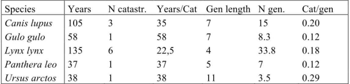
In table I, we have presented the five large carnivore species that appeared in the material of Reed et al. (2003). For wolf, three catastrophes had been reported for a combined time series of 105 years, i.e. one per 35 years or 0.20 per generation. Unfortunately, the authors did not give details for the different species, so we do not know the severity or the cause of the three catastrophes reported. Among the 96 catastrophes reported by Young et al. (1994), none concerned wolf, and only six concerned other species of large carnivores. There were three cases for African wild dog (Lycaon pictus) varying between 63 and 84 % mortality, two for coyote (Canis latrans) with a severity of 50 and 87 % respectively, and one for Lion ( Pan-thera leo) with 75% mortality. All cases but one were caused by disease.

Table I. Frequency of die-offs with 50% or higher mortality within 1 year in five taxa of large carni-vores (from Reed et al. 2003).

Species Years N catastr. Years/Cat Gen length N gen. Cat/gen

Canis lupus 105 3 35 7 15 0.20

Gulo gulo 58 1 58 7 8.3 0.12

Lynx lynx 135 6 22,5 4 33.8 0.18

Panthera leo 37 1 37 5 7 0.12

Ursus arctos 38 1 38 11 3.5 0.29

Murray et al. (1999) reports 7 cases of die-offs in wolves caused by disease, four by rabies, one by distemper and one by parvovirus. In one case it was unclear whether the causing agent was parvovirus or distemper. Mortality varied between 9 and 30 %, except for one case of rabies, where it was 60 %. This latter mortality regarded only one pack of ten wolves though. Apart from these cases we also know of one large die off on Isle Royale, where the population went down from 50 to 14 in 1980-82, i.e. a reduction with 72 % in two years (Peterson 1995). The causing agent was canine parvovirus (CPV). The disease persisted in the population for another six years causing high chronic mortality, until it suddenly disappeared. The population on Isle Royale has existed for more than 60 years, and this is the only catastrophic die-off reported for this population. We do not know whether the Isle Royale time series was included in the material of Reed et al. 2003, but find that unlikely. At present, the population is in very bad shape, consisting of only 9 ani-mals, of which maximum two are mature females. The present situation is probably

(17)

mainly caused by a combination of strong inbreeding and demographic stochastici-ty. The Scandinavian wolf population has now existed for 30 years without any catastrophic die-off.

Methodology overview

The question we have been asked in the assignment goes against the recommended use of population models. It is generally advised to interpret results in a qualitative (why, how, and what if questions) rather than in a strict quantitative (when, where and how much questions) way (Beissinger 2002). Furthermore, a consensus in the modelling literature recommends avoiding proposing firm numbers for viability levels (Reed et al. 2002). While we understand the need of quantitative require-ments by real-world policy makers, we urge readers to not over-interpret our con-clusions and to recognize that model outcomes are strongly dependent on their assumptions. By interpreting model findings as absolute numbers, one may find that a population size considered as viable with one model might not be viable with another model. It is important to understand that the dynamics of biological sys-tems (such as a population) is the stochastic result of complex, interacting and often non-linear feedbacks, which renders their absolute quantitative interpretation inappropriate (Pilkey & Pilkey-Jarvis 2007). This stands in contrast to many physi-cal systems, which show a deterministic dynamics and for which scientists are able to make extremely accurate quantitative predictions, e.g. the future positions of planets or the resistance of a bridge have very little, if any, quantitative uncertainty. Interpreting biological models as it is possible to interpret physical models, espe-cially to make real-world management decisions, is therefore hazardous both in the short-term as there is no guarantee these outputs are accurate and in the long-term as this spuriously may lead to a broader defiance against model-based inferences among society.

In an attempt to address the request we have been given, without breaking the ac-cepted practices of using models, we have developed three different population models with increasing level of structural complexity, each relying on different assumptions, data and methods (Figure 1). By using different models, we aim at delineating a pool of results which taken together should generate a more robust confidence. Note that using different models is not the same as accounting for un-certainty, which is done independently in each model. This approach is analogue to the one adopted by the International Panel of Climate Change where several cli-mate models and scenarios are considered (Randall et al. 2007). We start with a simple model; having as few assumptions as possible and using only population count data. We follow with a model of intermediate complexity that uses more detailed data on survival and reproduction. Finally, we present a more realistic model – but also based on a lot more assumptions taking the form of biological rules. Each model is presented in its own separate section and a final section pro-vides a synthesis of our findings.

(18)

Figure 1: Schematic representation of the three models developed in this report. All models are used to compute extinction risk and to estimate a MVP for the Scandinavian wolf population.

MO D EL 1 Count data

+

MO D EL 2

Mortality data Reproduction data Count data

+

MO D EL 3

Mortality data Reproduction data

Count data Biological Rules

(19)

Exponential growth model

Model description

Our first model is the simplest one as the population at year t+1 is the population at year t minus harvest at year t multiplied by growth rate λ:

Nt+1=

λ

⋅

(

Nt−Ht

)

There is actually no wolf-specific assumption in this model. In fact any population has a growth rate and the only assumption that we make here is very general and needed in viability analysis: we assume that it is possible to infer about the future by observing the past – an assumption also known as the “principle of uniformitar-ianism”. With this model, we run simulations to find out what is the most likely value of population growth rate λ to have the model fitting the observed data the best and then run forward simulations to investigate how likely are populations to become extinct according to its growth rate and its variation. Due to density-dependence, an increase in population size is expected to reduce growth rate and in turn to influence the viability of the population. However, density dependence is unlikely to be relevant for small populations that are well below their biological carrying capacity. The carrying capacity of wolves in Scandinavia is likely quite high because there is plenty of space and wild ungulate prey for larger wolf popula-tions on the Scandinavian Peninsula (Karlsson et al. 2007), and both Sweden and Norway have some of the highest moose / wolf ratios in the world (Sand et al. 2012). We therefore do not include density-dependence in this model and the fol-lowing ones. Similarly, we have assumed in all the three models that the population was isolated and there was neither immigration nor emigration.

We formalize this model in a hierarchical way, which is a particular statistical ap-proach that provides the advantage of formalizing in a coherent probabilistic framework both the ecological process and the observation process from which the data emerge. In our case, the ecological process is the dynamics of the wolf popula-tion in Scandinavia, e.g. the survival and reproducpopula-tion of packs and wolves that lead to a population growth (or decline). The observation process is the winter census carried out nation-wide by field teams and we used population counts from 1999 to 2011 because their quality was consistent and better than data for previous years. The simulations explicitly consider that the model is not perfect, i.e. we cannot predict with absolute certainty what is going to be the wolf population size next year. The simulations will also explicitly consider that the census data are not the truth but have some error that may vary in size between years. For example the data tells us that population size in December 2010 was 277 wolves, but we con-sider this is an estimate and the true population (which remains unknown) may actually have been 270 or 290 wolves. Accounting for this observation error (either underestimates or overestimates of wolf population sizes) may lead to a more un-certain prediction but is important because it is the true population size (and not its estimate), which should be viable. While this may sound as artificially introducing

(20)

noise in the data, this is actually the correct way to proceed and ignoring observa-tion error is a mistake that can lead to spurious conclusions (Freckleton et al. 2006). We consider however that harvest data are perfectly observable. The results that we get are not a single value of λ, but rather a probability distribution of λ, indicating which values are more likely than others, but also which other values are still possible.

When written in a hierarchical way, we need to separate the process model and the observation model. The process equation is:

µt=log

(

λ⋅Nt−1−Ht−1

)

Ntlognormal

(

µt,σproc

)

⎧ ⎨ ⎪ ⎩⎪

where µt is the deterministic prediction of the median wolf population size at time t, Nt is the true population size at time t, σproc is the standard deviation of the true

population size on the log scale, λ is the yearly population growth rate. The process equation is linked to data using the observation equation:

αt= Nt 2 σNobs 2 βt= Nt σNobs 2 ψtgamma

(

αt,βt

)

NobstPoisson

( )

ψt ⎧ ⎨ ⎪ ⎪ ⎪⎪ ⎩ ⎪ ⎪ ⎪ ⎪

where Nobst is the observed population size at time t, σNobs is the estimate of the

error of observation of the population size. This formulation views the count data hierarchically – the mean observed count of wolves at time t is Poisson distributed with mean ψt and this mean is drawn from a gamma distribution with mean equal

to the prediction of the process model and a standard deviation for observation error. We estimate the posterior distribution of each parameter by running Monte-Carlo Markov chains (MCMC), implemented in JAGS (Plummer et al. 2003) with R (R Development Core Team 2009). Three chains were initialized with different sets of parameter values chosen within biologically plausible bounds. After an initial burn-in period of 100,000 iterations, we obtained 1,000,000 iterations of each of the chains, thinning each by 10. We successfully checked for convergence using the Heidelberger & Welch stationarity and half-width tests with the CODA package (Plummer et al. 2006).

In order to compute MVP, we need to run simulations that will project the popula-tion dynamics into the future. We do this by considering that during the next 100 years, population growth rates are going to be drawn from the same probability distribution as the one they have been drawn from during the past 10 years – i.e. the posterior density we just obtained by MCMC sampling. This way we keep all uncertainty from parameters to MVP estimates. We model process error or

(21)

demo-graphic stochasticity by a Poisson function instead of the parameter σproc because

we need to have integers for counting individuals. Environmental stochasticity is accounted for in the posterior distribution of λ.

Since we want to infer about a MVP, we cap the population at a ceiling K (consid-ered as a maximum population size implemented by harvest) and we run Monte Carlo simulations (100,000 trajectories) with various values of K (K being constant during each simulations) and compute each time the resulting probability of extinc-tion. The smallest value of K that leads to an extinction probability lower than 10% (or 5% when indicated) is the MVP.

Model assessment

Our simulations indicate that the Scandinavian wolf population has been growing at a median annual rate of λ = 1.18±0.02 during the period 1999-2011 (Figure 2). Worth clarifying is that this growth rate is not the realized growth rate but the po-tential one because harvest data is included in the model. In other words, we esti-mate the most likely growth rate the population would have shown if no harvest had taken place. Note also that our results take the form of a distribution of values and not of a point estimate: while our data supports the most a λ of 1.18, uncertain-ty in the process and the shortness of the time series indicate that there is also some support, but weaker, for other values of λ such as 1.16 or 1.20. The shape of the distribution indicates that the probability of having λ <1 is almost equal to 0.

Figure 2: Posterior distribution of growth rate λ estimated by fitting an exponential growth model to the 1999-2011 time series of the Scandinavian wolf population. The most likely value for λ is 1.18 and the standard deviation is 0.02.

1.05 1.10 1.15 1.20 1.25 1.30 1.35 0 5 10 15 20 25 Growth rate Probability density

(22)

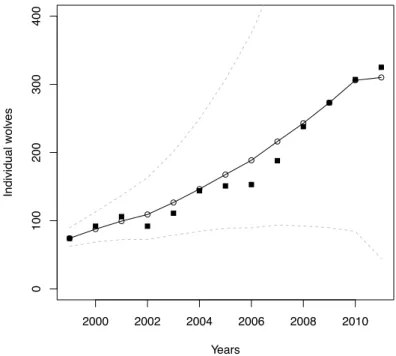
We can evaluate how well our model is able to explain our data by running simula-tions starting with the population size in 1999 and ran until 2011 (and considering the harvest that took place). We find that the model correctly matches the data (Figure 3) and this reveals that the distribution of the growth rate we have comput-ed is able to well capture the population dynamics of wolves in Scandinavia during the past 12 years. However, Figure 3 also reveals that there is a wide standard de-viation (shown by the dashed lines) and that the further the simulation moves for-ward in time, the less precise its forecast becomes. We are able to estimate well the median population size 12 years ahead (it is in fact almost the same as the observed data) but the standard deviation of the predicted population in 2011 is ±96 wolves. This is something important to be aware of because MVP computations consist in forward simulations lasting 100 years and have a very high uncertainty.

Figure 3: Forecasting simulation starting from 1999 with the exponential growth model (λ = 1.18±0.02). The black squares are annual census data of the Scandinavian wolf population, the open circles are the median population size predicted from the model and the dashed lines indi-cates ± standard deviation of our model predictions. Notice how this standard deviation becomes extremely large after just a few years of simulation.

Computations of MVP

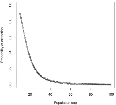
When capping population size, stochastic simulations show that a wolf population with the same growth rate as the one of the Scandinavian population has an extinc-tion risk less than 10% (resp. 5%) if it is capped at 22 individuals (resp. 25 individ-uals) (Figure 4). In other words, culling all surplus individuals above a threshold of 22 or 25 individuals does not lead to an extinction risk higher than 10% or 5% according to this model and its assumptions.

● ● ● ● ● ● ● ● ● ● ● ● ● 2000 2002 2004 2006 2008 2010 0 100 200 300 400 Years Individual w olv es

(23)

Figure 4: Extinction probability as a function of population cap for a theoretical population having the same parameters (λ = 1.18±0.02) as the ones of the Scandinavian wolf population. Horizontal grey lines are 5% (dashed) and 10% (continuous) threshold of extinction risk.

Future scenarios

The former result is particularly dependent on the limiting assumption that the probability distribution of the population growth rate of the Scandinavian wolf population will remain the same for the next 100 years as it is today. This assump-tion is unlikely to be true because if there is anything we can be sure of, it is that the future is not going to be exactly like the past. We are not considering possible density dependent effects here – which would be unlikely in such a small popula-tion – but rather possible changes in habitat, prey base or simply human attitudes. We can envision two general kinds of changes: gradual ones (change of growth rate and its variation, Boyce 1992) or new events that have never happened before (catastrophes, Albon et al. 2000).

To investigate how the population cap (i.e. the MVP level) needs to be adjusted to these possible changes, we now run simulations but with different values of growth rate and its variation. We consider all cases: growth rates from 1.00 to 1.30 and growth rate standard deviation (SD) from 0 to 0.10. For each λ and its SD, we es-timate the required MVP (Figure 5) by running 10,000 runs of a Monte Carlo simu-lation. The only difference from the previous simulation is that here growth rate is no longer drawn from the distribution we estimated with the hierarchical model fitted to Scandinavian data, but from a normal distribution (excluding negative values as we assume λ > 0) whose parameters are mean λ and its SD.

● ● ● ● ● ● ● ● ● ● ● ● ● ●_● ●●● ●●●●●●●●●●●●●●●●●●●●●●●●●●●●●●●●●●●●●●●●●●●●●●●●●●●●●●●●●●●●●●●●●●●●●●●●● 20 40 60 80 100 0.0 0.2 0.4 0.6 0.8 1.0 Population cap Probability of e xtinction

(24)

Figure 5. Theoretical MVP contour curves (left panel: with extinction risk < 5%, right panel: with extinction risk < 10%) for an exponential growth model as a function of growth rate λ and its standard deviation. The empty square indicates the actual Scandinavian wolf population (λ = 1.18±0.02), black squares indicate other wolf populations (Wisconsin: λ = 1.16±0.02, Michigan: λ

= 1.26±0.07, Montana: λ = 1.20±0.07, Wyoming: λ = 1.21±0.1, Idaho: λ = 1.34±0.1, data from USFWS).

Figure 5 shows that populations experiencing growth rates typical of recovering wolf populations (λ > 1.15 and SD < 0.1) remain viable if they are capped at 30 individuals or more. Considering an acceptable extinction risk of 10%, the parame-ters at which a wolf population capped at 40 individuals is not viable are for exam-ple λ < 1.07 with no variability (SD = 0.0) or λ < 1.09 with a high variability (SD = 0.10). Considering an acceptable extinction risk of 5% instead of 10% generates only small increases in viability levels. Populations appear to be more resilient to increased environmental variation than to decreased baseline growth rate since the contour curves on Figure 5 have a vertical alignment pattern. In other words, a small change on the lambda axis is more likely to require a change in MVP than a corresponding small change on the SD axis is.

Effects of catastrophes

Another way the future can be different from the past is when catastrophes – rare events but with a high impact – occur. There is no obvious satisfying way to model catastrophes as one faces the challenge of estimating the probability of occurrence of an event that has rarely or never occurred before. We circumvent this obstacle by considering many possibilities and adopting an inverse reasoning. Rather than guessing catastrophe patterns, we compute what would be their required frequency and intensity to have the actual Swedish wolf population not viable (with its actual growth rate). We find that a population capped at 30 wolves has an extinction risk lower than 10% even when facing catastrophes from one every decade reducing the population by up to 40% of the population at each occurrence or a catastrophe every century reducing the population by 70% (Figure 6). For a population capped at 100 individuals to not be viable, it would need to face for example one catastro-phe every decade reducing the population by more than 60% of the population, or

Median of growth rate

SD of gro wth r ate 20 30 40 50 100 150 200 1.00 1.10 1.20 1.30 0.00 0.02 0.04 0.06 0.08 0.10

Median of growth rate

SD of gro wth r ate 20 30 40 50 100 150 200 1.00 1.10 1.20 1.30 0.00 0.02 0.04 0.06 0.08 0.10

(25)

one catastrophe every century killing almost the whole population (in which case no population can actually be viable).

Figure 6: MVP contour curves (with extinction risk of 10%) as a function of frequency of catastro-phes (one per century = 0.01, one per decade = 0.1) and of intensity (reducing population size by 1% up to 90%) for a theoretical population having the same parameters (λ = 1.18±0.02) as the ones of the Scandinavian wolf population.

Frequency of catastrophes Intensity of catastrophes 20 30 40 50 100 250 500 1000 0.00 0.02 0.04 0.06 0.08 0.10 0.0 0.2 0.4 0.6 0.8

(26)

Bayesian model

Model description

While the strength of the previous model was its relative simplicity, its drawback was its limited use of available data. During the past 13 years, the Scandinavian Wolf Project has been able to collect one of the most comprehensive dataset of wolves in the world. This data can be instrumental in leveraging our understanding of wolf population dynamics and consequently in estimating possible levels of MVP. The second model we develop is therefore a model whose strength relies on its ability to merge multiple sources of data and prior information in a streamlined way. This model belongs to the family of integrated hierarchical Bayesian state-space models and is actually an extension of the previous model. We modify the first model to include other available data and then run similar computations. While the previous model considered that population at year t+1 was the popula-tion at year t minus harvest at year t multiplied by growth rate λ, this new model considers that population at year t+1 is the outcome of births and deaths occurring during year t. This is also a very general model as any population of individuals experience births and deaths at any time step and the result becomes the updated population. We did not include density dependence in this model (see previous model). The model can be written:

N

_t₊₁

=

(

1−

m

)

⋅

N

_t

+

f

⋅

R

_t

−

H

_t

where m is mortality rate, f is litter size and Ht is harvest at time t. We can infer

growth rate from the model with λ = (1 - m) + a where a is per-capita reproduction rate estimated from f. The model is also written in a hierarchical way, similar to the previous model and also considering observation errors. The additional data we include compared to the first model is annual number of reproductions Rt. We also

include prior knowledge in the model by giving informative priors to parameters. We run a Kaplan Meier analysis to compute annual mortality from radio-telemetry data and use the median mortality estimate ± SD as an informative prior to mortali-ty m. From reproduction data, we calculate a median litter size estimate ± SD and use it as an informative prior to litter size f.

We estimate the posterior distribution of each parameter – in particular m, f and a – by running Monte-Carlo Markov chains, implemented in JAGS (Plummer et al. 2003) with R (R Development Core Team 2009). Three chains were initialized with different sets of parameter values chosen within biologically plausible bounds. After an initial burn-in period of 100,000 iterations, we obtained 1,000,000 itera-tions of each of the chains, thinning each by 10. We successfully checked for con-vergence using the Heidelberger & Welch stationarity and half-width tests with the CODA package (Plummer et al. 2006).

As with the first model, we need to run simulations that will project the population dynamics into the future to compute MVP. We do this by considering that during the next 100 years, mortality and per-capita reproduction rates are going to be

(27)

drawn from the same probability distributions as the one they have been drawn from during the past 10 years. We model both demographic and environmental stochasticities by a binomial distribution for survival and by a Poisson distribution for reproduction. Since we want to infer about a MVP, we cap the population at a ceiling K (considered as a maximum population size implemented by harvest) and we run Monte Carlo simulations (100,000 trajectories) with various values of K (K being constant during each simulations) and compute each time the resulting prob-ability of extinction. The smallest value of K that leads to an extinction probprob-ability lower than 10% (or 5% when indicated) is the MVP.

Model assessment

Simulations indicate that our data supports the most a mortality rate m = 0.24±0.02 and a (winter) litter size f = 4.29±0.47, which corresponds to a per-capita reproduc-tion rate a = 0.42±0.05. When converted into a population growth rate, these values indicate the population has had an annual growth rate of λ = 1.18 which is exactly the same value obtained with the independent first model.

Figure 7: Forecasting simulation starting from 1999 with the Bayesian model (m = 0.24±0.02 and

a = 0.42±0.05). The black squares are annual census data of the Scandinavian wolf population, the open circles are the median population size predicted from the model and the dashed lines indicates ± standard deviation of our model predictions. Notice how this standard deviation be-comes extremely large after just a few years of simulation.

Simulations starting with the size of the wolf population in 1999 as initial popula-tion and running for 12 years until 2011 are able to correctly match the data (Figure 7). However, and same as with the previous model, we find that there is a large standard deviation of our predictions (shown by the dashed lines) and that the

fur-● ● ● ● ● ● ● ● ● ● ● ● ● 2000 2002 2004 2006 2008 2010 0 100 200 300 400 Years Individual w olv es

(28)

ther the simulation moves forward in time, the less precise its forecast becomes. While the second model uses more data and considers wolf population dynamics at a finer scale (i.e. deaths and births rather than only growth rate), we still have a wide uncertainty when predicting population size a few years ahead, and this un-certainty can only become much larger when predicting one century ahead.

Computations of MVP

When capping population sizes, stochastic simulations show that a wolf population with the same annual mortality rate and per-capita reproduction rate as the ones of the Scandinavian population has an extinction risk less than 10% (resp. 5%) if it is capped at 33 individuals (resp. 42 individuals) (Figure 8). In other words, culling all surplus individuals above a threshold of 33 or 42 individuals does not lead to an extinction risk higher than 10% or 5% according to this model and its assumptions. The difference of values between the current and the previous model arises from the fact that the current model describes the wolf population dynamics with finer details by discriminating between two stochastic processes (i.e. survival and repro-duction).

Figure 8: Extinction probability as a function of population cap for a theoretical population having the same parameters (m = 0.24±0.02 and a = 0.42±0.05) as the ones of the Scandinavian wolf population. Horizontal grey lines are 5% (dashed) and 10% (continuous) threshold of extinction risk.

Future scenarios

With this model, we also consider how changes in demographic and environmental conditions may affect population viability. We investigate how MVP levels need to

● ● ● ● ● ● ● ● ● ● ● ● ● ● ● ●● ●● ●● ●●_●●● ●●●●●●●_{●●●●●●●●●●●●●●} ●●●●●●●●●●●●●●●●●●●●●●●●●●●●●●●●●●●●●●●●●●●● 20 40 60 80 100 0.0 0.2 0.4 0.6 0.8 1.0 Population cap Probability of e xtinction

(29)

be adjusted to changes in mortality by running simulations but with different values of mortality rate. We only studied the effect of mortality, as changes in mortality rate has the largest impact on growth rate for large carnivores, i.e. long-lived spe-cies. For normally distributed mortality ranging from 0.1 to 0.5 and with the same SD as the one of the posterior distribution of m, we estimate the required MVP by running 10,000 runs of a Monte Carlo simulation for each mortality rate (Figure 9). We find that no population can be viable (for 100 years) if its mortality rate is 42% or higher – extinction is then deterministic. Note that mortality rates slightly small-er than 42% are still likely to lead to extinction, these simulations do not show this because some populations have not yet gone extinct within 100 years. For the Scandinavian population, having a mortality rate of 24%, a population cap of 30 individuals is sufficient to keep extinction risk below 10%.

Figure 9: Extinction probability contour curves as a function of mortality rate and population cap (MVP). The actual mortality rate of the Scandinavian population (m = 0.24) is shown by the con-tinuous vertical line. No population is viable if m > 0.42 (dashed vertical line).

Effects of catastrophes

When simulating catastrophes, we find that a population capped at 30 wolves has an extinction risk lower than 10% even when facing catastrophes from every dec-ade and reducing the population by up to 15% of the population at each occurrence or a catastrophes every century reducing the population by 40% (Figure 10). For a population capped at 100 individuals to not be viable, it would need to face for example one catastrophe every decade reducing the population by more than 60%, or one catastrophe every century removing almost all the population (in which case no population can actually be viable).

Average mortality rate

P opulation cap 0.05 0.1 0.25 0.5 0.1 0.2 0.3 0.4 0.5 0 20 40 60 80 100

(30)

Figure 10: MVP contour curves (with extinction risk of 10%) as a function of frequency of catas-trophes (one per century = 0.01, one per decade = 0.1) and of intensity (reducing population size by 1% up to 90%) for a theoretical population having the same parameters (m = 0.24±0.02 and a

= 0.42±0.05) as the ones of the Scandinavian wolf population. Irregular patterns are stochastic artefacts. Frequency of catastrophes Intensity of catastrophes 30 40 50 75 ₁₀₀ 0.02 0.04 0.06 0.08 0.10 0.0 0.2 0.4 0.6 0.8

(31)

Individual

-

based model

Model description

General approach

The two previous models were not wolf specific and could have been used to mod-el the viability of any population. Any population has a growth rate and experienc-es deaths and births of individuals. The only wolf specific elements in thexperienc-ese models were parameters that we estimated by Bayesian inferences. Another method to address viability questions in ecology is to develop more realistic models – based on high quality data – which try to capture with some degrees of realism what ac-tually happens in the lives of animals (Case 2000). These models can be age-structured where one describes the survival and reproduction rates for age-related classes of individuals. This is the basis of Leslie matrices and is the approach also followed by the packaged model VORTEX (with demographic, environmental and genetic stochasticities further included, Lacy 1993 & 2000). More realism can be brought by considering stage-structured models where classes of individuals can consider for example social status. However, the field of viability modelling has recently benefited from a conceptual and methodological improvement with the introduction of rule-based models – more often termed individual-based models (Grimm et al. 2005). Because the model is ruled-based, it can have the individual (or a pack or a pride) as its functional unit and this allows consideration of more explicit biological realities. Individual-based models can consider much more than random events in survival or fecundity since individuals or packs can be tracked during the whole simulation with dynamically varying parameters such as spatial aspects, behaviour, or social mechanisms. Because the model considers mecha-nisms at the individual or pack level, the demographic consequences of these mechanisms are population level emerging properties of the model and are not predefined by equations as in more traditional population models (as they were in the previous two models).

Using an individual-based model, as opposed to traditional age-class models, is a particularly relevant choice when modelling wolf population dynamics. The wolf is a social animal living in packs, which is in fact the functional unit of a wolf popu-lation. Events at the individual and pack levels – e.g. dispersing from a natal pack, founding a new pack – shape the overall population dynamics. In addition, killing individuals has different effects if this individual is a pack breeder or a

non-breeding animal. We have developed a wolf specific rule-based model where every wolf is described as an “object” (in a computer programming sense) and character-ized by its biological “attributes” (sex, social status, pack, age, etc.) and where every pack is also described as an “object” with attributes (breeding male and fe-male, litters, etc.). The rules governing how individuals and packs react to events have been constructed and parameterized from the long-term biological data of the Scandinavian Wolf Project. Also in this model, we did not include density depend-ence (see above). The model is coded in Objective-C and compiled with CLANG

(32)

in Xcode 4.3. It uses the GNU Scientific Library for probability arithmetic, libdis-patch for multi-threading and the Mersenne Twister random number generator.

Algorithms

The model runs Monte Carlo simulations by repeating 10,000 random trajectories, each of them starting by the creation of a fixed initial number of packs containing each a dominant couple. The time step in the model is one month and wolves in the simulated population go through particular events according to their sex, status, pack membership or age. Every month, all individuals survive or die following a Bernoulli trial drawn from a monthly survival probability normally distributed with same shape parameters of the posterior distribution of survival rate estimated in the previous model (mortality rate m = 0.24±0.02). In this way, we include both demo-graphic (Bernoulli trial) and environmental stochasticities (posterior sampling). Non-reproducing individuals in packs (i.e. young of previous year litters) disperse to become transients or remain in their pack following a Bernoulli trial drawn from a monthly dispersal probability estimated from empirical data of the Scandinavian wolf population (Wabakken, unpubl. data). When the breeding couple in a pack dies, all other members of the pack automatically disperse to join the pool of tran-sients and the pack ceases to exist and is removed from the population. Every month, transients will try to find a transient mate of the opposite sex and to settle on a vacant territory. Transients also try to settle in packs where a same sex breeder is missing. Production of litters in packs is modelled by sampling from a Poisson distribution, whose parameter is itself drawn from a normal distribution of litter size with same shape parameters of the posterior distribution of litter size estimated in the previous model (f = 4.29±0.47). Similar to survival, we include in this way both demographic (Poisson trial) and environmental stochasticities (posterior sam-pling). Winter population count is implemented one time per year (in December).

Simulations

Except for the simulation to evaluate whether the model can match well the ob-served Scandinavian wolf population growth, we include a population ceiling, which is the MVP. We define the MVP in individuals and any individual above the ceiling is automatically removed. When removing individuals, all adult wolves have a probability to be removed and random Bernoulli trials are performed until the population is back at its ceiling.

Model assessment

We evaluate the model by confronting it with summary statistic of several wolf populations in the world. We run simulations to compute the growth rate of wolf populations with median mortality rate ranging from 0.15 to 0.75. We compare the simulated growth rates with values obtained for field studies of several wolf popu-lations (note that contrarily to the two previous models, we do not fit this model to these data, because cannot write its likelihood). We find that the model captures well the dynamic of most wolf populations (Figure 11). All of them (except for low

(33)

mortality) are within the 95% confidence interval. The model predicts larger growth rates for low mortality rates than the empirical data and this is likely due to the fact that real-wolf populations were close to carrying capacity, which is not the case for simulated data.

Figure 11: Population growth rates computed by the model as a function of mortality rate (which is the same for all wolves). Continuous black line is median of simulations, dashed is ±SD and black dots are data from different wolf populations worldwide (see Marescot et al. 2012 for details).

We also simulate for 32 years the trajectory of a wolf population starting with 1 pack. We find that the model matches relatively well the observed growth of the Scandinavian population from 1980 to 2012 (Figure 12). The model does not fit the data as well as the previous models because here we cannot run MCMC simula-tions, the model being individual-based, writing its likelihood is intractable. In addition, the model does not consider harvest events.

● ● ● ● ● ● ● ● ● ● ● ● ● ● ● ● ● ● ● _{● ● ● ●} ● ● 0.2 0.3 0.4 0.5 0.6 0.7 0.0 0.5 1.0 1.5 2.0 Mortality rate P opulation gro wth r ate

(34)

Figure 12: Forecasting simulation starting from 1980 with the individual-based model. The black squares are annual census data of the Scandinavian wolf population, the open circles are the median population size predicted from the model and the dashed lines indicates ± standard devia-tion of our model predicdevia-tions. As with previous models, notice how this standard deviadevia-tion be-comes extremely large after just a few years of simulation.

Computations of MVP

When capping population size, stochastic simulations show that a wolf population with the same annual mortality rate and per-capita reproduction rate as the ones of the Scandinavian population has an extinction risk less than 10% (resp. 5%) if it is capped at 38 individuals (resp. 41 individuals) (Figure 13). In other words, culling all surplus individuals above a threshold of 38 or 41 individuals does not lead to an extinction risk higher than 10% or 5% according to this model and its assumptions. These values are remarkably similar to the much simpler previous models.

● ● ● ● ● ● ● ● ● ●● ● ● ● ●● ● ●● ● ● ● ● ● ● ● ● ● ● ● ● ● 1980 1985 1990 1995 2000 2005 2010 0 50 100 150 200 250 300 350 Years P opulation siz e

(35)

Figure 13: Extinction probability as a function of population cap for a theoretical population with parameters (mpack = 0.24±0.02 and f = 4.29 ±0.47) obtained from the Scandinavian wolf

popula-tion. Horizontal grey lines are 5% (dashed) and 10% (continuous) threshold of extinction risk.

Future scenarios

We investigate how MVP levels need to be adjusted to changes in mortality by running simulations but with different values of mortality rate. For mortality rang-ing from 0.1 to 0.5, we estimate the required MVP (Figure 14) by runnrang-ing 1,000 runs of a Monte Carlo simulation. We find that no population can be viable during 100 years if its mortality rate is 39% – where extinction is deterministic. Note that mortality rates slightly smaller than 39% are still likely to lead to extinction, these simulations do not show this because some populations have not yet gone extinct within 100 years. For the Swedish population, having a mortality rate of 24%, a population cap of 30 individuals results in an extinction risk below 10%.

●●●●●●● ● ● ● ● ● ● ● ● ● ● ● ● ● ● ● ● ● ● ●●_● ●●● ●●●●● ●●●●●●●●●●●●●●●●●●●●●●●●●●●●●●●●●●●●●●●●●●●●●●●●●●●●●●● 20 40 60 80 100 0.0 0.2 0.4 0.6 0.8 1.0 Population cap Extinction probability

Demographic Viability of the Scandinavian Wolf Population