Chapter 2. Theoretical framework

(1)

Chapter 2 Theoretical framework

For studying the properties of thin films and surfaces on the atomic scale a wealth of experimental techniques is available. For brevity, we will in-troduce only those that will be of particular importance for thin insulator films and the questions addressed in this work. For developing a micro-scopic understanding of a material, the atomic structure is of fundamental interest. Crystalline materials are investigated by the diffraction of photons (X-ray diffraction, XRD), electrons (low-energy electron diffraction, LEED), and ions (low energy ion scattering, LEIS). Further insight, also for non-crystalline materials, can be gained by microscopies that reach atomic res-olution, such as scanning tunnelling microscopy (STM) or atomic force mi-croscopy (AFM). Indirect, but often invaluable information is deduced from other experimental data since many properties are strongly correlated to the local atomic structure. For example the vibrational spectrum can exhibit frequencies that are characteristic for certain atomic configurations such as hydroxyl groups. The phonon spectrum is measured by infrared (IR) spec-troscopy, Raman specspec-troscopy, and also by high-resolution electron energy loss spectroscopy (HREELS).

A second key property is the electronic structure. While the knowledge of the electronic ground state is sufficient to describe the techniques described above, the electronic structure reveals itself only when excited. We can group the experimental techniques into those where the excited electrons remain in the sample such as optical spectroscopy in the visible and ultraviolet range (UV-VIS) or electron energy loss spectroscopy (EELS), and electron spec-troscopies that change the number of electrons. Of particular importance is photoelectron spectroscopy (PES) where electrons are excited from the sample by electromagnetic radiation. Depending on the energy of the pho-tons, one distinguishes between ultraviolet photoelectron spectroscopy (UPS) for the valence electrons and X-ray photoelectron spectroscopy (XPS) for

(2)

Chapter 2 Theoretical framework

the core electrons. The inverse process (inverse photoelectron spectroscopy, IPES), i.e. the emission of photons when electrons are added to the system (bremsstrahlung isochromat spectroscopy, BIS), yields information about the unoccupied part of the spectrum. Also excited He atoms can be used to excite electrons (metastable impact electron spectroscopy, MIES).

The primary experimental data often provide only indirect information about the properties of interest, which must then be deduced from the exper-imental data by analogy to known systems (“empirical knowledge”). Usually, experimental results from several techniques must be combined to arrive at a consistent picture of the atomic scale. In this situation, theory can supple-ment the experisupple-ment in various ways. In addition to the empirical knowledge, appropriate theories help to assign experimental features to the correspond-ing microscopic structures or processes. Theoretical simulations can also add data not available from experiment such as the microscopic energetics, the electron distribution, the bonding behaviour, or the character of electronic states. Theory can thereby refine, validate, and sometimes reject the mod-els proposed on the basis of experimental results. The increase in computer power has even made it possible to develop completely new models from extensive theoretical simulations to explain available experiments. The com-bination of theory and experiment has proved to be a powerful tool to solve complex questions in surface science. For this it is necessary to employ and develop ab initio _{theories that accurately describe the experimental results}

without relying on experimental input. To address the questions mentioned in the introduction, we have employed density functional theory and many-body perturbation theory in theGW approximation. These will be described in the following.

The physics at the atomic scale is governed by the principles of quantum mechanics. A system of atomic nuclei and electrons is described quantum-mechanically by its wavefunction Ψ, which depends on the coordinates of all electrons (indexed by i, j . . .) and all nuclei (indexed by µ, ν . . .). It solves the time-independent Schr¨odinger equation

HΨ(xi,Rµ) =E Ψ(xi,Rµ), (2.1)

whereE denotes the total energy of the system and the Hamiltonian is1

1_{In the following, Hartree atomic units are used, i.e. ¯}_h₌_m

(3)

Theoretical framework Chapter 2

According to the Copenhagen interpretation of quantum mechanics, the ab-solute square of the wavefunction is proportional to the probability density of finding a particle at each of its arguments. Particles of the same kind (e.g. electrons or identical nuclei) are indistinguishable. When two elec-trons (or other fermions) are exchanged, the wavefunction changes its sign (anti-symmetry) whereas it is symmetric with respect to boson exchange.2

Taking into account that the electrons are lighter than the nuclei by three to four orders of magnitude, we can employ the Born-Oppenheimer approximation [33]: assuming that the electrons adapt instantaneously to any movement of the nuclei, the motion of the electrons can be decoupled from that of the nuclei. For each atomic configuration, the electronic Schr¨odinger equation then reads

 − X i 1 2∇ 2 i − X i,µ Zµ |ri−Rµ| +X i<j 1 |ri−rj|  Ψ(x_i) =Eel(R_µ)Ψ(xi). (2.3)

The nuclei appear here only as the point charge sources of the electrostatic potential in which the electrons move. For generality, this potential will be denoted as the external potential Vext in the following.

For the movement of the nuclei, only the electronic energy as a function of the nuclear positions is required. Including the internuclear repulsion (and possibly external fields acting on the nuclei), this is called the potential energy surface. An important task of simulations is to find and characterise minima on this potential energy surface since they correspond to the stable atomic structures. The nuclei in the real world are of course never at rest due to their quantum nature and thermal fluctuations. This does not harm the concept of an atomic structure because usually the nuclei fluctuate around the Born-Oppenheimer minimum. The structural parameters obtained from experi-ments that probe the average positions should thus in a first approximation correspond to the theoretically computed minimum-energy structures. Zero-point vibrations and the anharmonicity of the potential energy surface lead to small (_∼0.5%) deviations. The movement of the nuclei is also neglected for electronic excitations (Franck-Condon principle), which appears justified for the photoemission processes. We therefore assume that the nuclei remain in their ground-state positions during the excitation process.

Even the electronic Schr¨odinger equation cannot be solved for realistic systems that contain dozens to thousands of electrons3_{. Moreover, the}

knowl-2_{Bosons are particles with an integer spin while fermions have an half-integer spin.} 3_{Of course, a macroscopic object has}_∼₁₀23 _{electrons, but a fully quantum-mechanical} description of such an object is neither feasible nor appropriate. The theoretical models must therefore be restricted to a small relevant part such as a cluster or the unit cell of a perfect crystal.

(4)

Chapter 2 2.1. Density functional theory (DFT)

edge of the full wavefunctions is not required since experiment and simplifying theories probe only certain aspects of the wavefunction. Further simplifying approximations have to be made to the solution of the Schr¨odinger equa-tion to drastically reduce the complexity and simplify the computaequa-tion. As sketched out above, many properties depend on the electronic ground-state energetics. For this purpose, density functional theory (DFT), which builds on the ground-state electron density as the basic variable, provides an excel-lent choice. We will describe it in Section 2.1. From the DFT calculation, we extract experimentally observable quantities e.g. the atomic structure, the mechanical and elastic properties, the formation energy of compounds and many more. However, for a comparison with photoelectron spectroscopy we have to go beyond ground-state DFT4_{. An appropriate framework is Green’s}

function theory, in particular many-body perturbation theory (MBPT) in the GW approximation (GWA). The GWA has been shown to describe the valence electron spectra in good agreement with experiment for many weakly correlated bulk systems such as the main group semiconductors and simple metals [23]. The GWA has also been applied to the surfaces of these mate-rials with some success. We will describe the GWA and its connection with photoelectron spectroscopy in Section 2.3. In Section 3, the application of

GW for surface and slab systems will be reviewed, highlighting critical points that have been neglected so far.

2.1 Density functional theory (DFT)

In this Section we will present density-functional theory in the Kohn-Sham (KS) formalism for the electronic ground state and furthermore discuss how the outcome of a DFT calculation can be compared to experimental results. In density-functional theory, the electronic many-body problem (Eq. 2.3) is reduced to finding the electronic ground-state energy without formally including all the electronic degrees of freedom. Instead, the electron density

n(r) =

Z

d3r1d3r2. . . d3rN |Ψ(r1,r2, . . . ,rN)|2δ(r−r1) (2.4)

is used as the basic variable. Hohenberg and Kohn have proved that for a system with a non-degenerate groundstate, there exists a one-to-one map-ping between the ground-state density and the external potential (up to a constant) in which the electrons are moving [34]. A more constructive proof

4_{Although in DFT every aspect of the electronic system is a functional of the} ground-state electron density in principle, the focus in practice is on the ground-ground-state total energy functional and derived quantities.

(5)

2.1. Density functional theory (DFT) Chapter 2

that also includes degenerate ground-states is due to Levy [35]. Since the external potential defines the electronic Hamiltonian uniquely, all electronic properties are uniquely defined from the ground-state density, too. The elec-tronic energy of the system is thus a functional of the electron density. The true ground-state density minimises this global functional for a given external potential. However, its functional form is not known explicitly.

Kohn and Sham have further shown that the electron density n(r) can be reproduced by a fictitious system of non-interacting electrons moving in an effective field [36]. We denote the normalised, orthogonal one-electron wavefunctions by φi. The antisymmetric many-electron wavefunction of N

non-interacting electrons takes the form of a Slater determinant

Ψ(r1. . .rN) = X P χ(P) N Y i=1 φi(rP(i)) (2.5)

where the sum runs over all permutations P of N numbers and χ(P) is the character of the permutation (+1 for even, -1 for odd permutations). The density is then obtained from the occupied5 _{one-particle wavefunctions}_φi _as

n(r) = X

i

|φi(r)_|2 . (2.7)

From the density, the Hartree energy, the classical repulsion of the charge distribution, EH = 1 2 Z d3r Z d3r′ n(r)n(r′) |r₋r′_| (2.8)

and the potential energy in the external field

Eext =

Z

d3_{r n}₍_r₎_V

ext(r) (2.9)

can be obtained.

The advantage of the Kohn–Sham approach lies in the fact that a large part of the kinetic energy can be recovered by the kinetic energy Ts of the non-interacting electrons Ts[φi] =− 1 2 X i hφi_|∇2_|φi_i, (2.10)

5_{At zero temperature, the electron states are either occupied or unoccupied. For metals,} it is numerically advantageous to assume an artificial temperatureT. The states are then occupied according to the Fermi partition

fi=

1

1 +e(ǫi₋µ)/(kBT) (2.6)

whereµis the Fermi energy andkB the Boltzmann constant. All state summations then

(6)

Chapter 2 2.1. Density functional theory (DFT)

which is an explicit functional of the one-particle wavefunctions. Kohn and Sham proposed to separate of the electronic energy into the following contri-butions

Eel =Ts[φi] +EH[n] +Exc[n] +Eext[n], (2.11)

where the exchange-correlation energyExccontains everything that is missing

from the previous terms, notably the exchange energy, the correlation energy, but also the difference between the true kinetic energy andTs. It also cancels

the self-interaction contained in the Hartree energy.6 _{Approximations to this}

exchange-correlation functional will be discussed below.

For the Kohn-Sham functional (Eq. 2.11), the variational principle ap-plies, i.e. the ground state assumes the minimum of the functional. The variational derivatives of the explicitly density-dependent terms in Equa-tion 2.11 with respect to the density, i.e. the Hartree potential

VH(r) = δEH δn(r) = Z d3r′ n(r′) |r₋r′_| , (2.12)

the exchange-correlation potential7

Vxc(r) =

δExc[n]

δn(r) , (2.13)

and the external potential can be combined into one local effective potential

Veff(r) = VH(r) +Vxc(r) +Vext(r). (2.14)

Minimisation with respect to the orbitals φi under the constraint that these stay orthonormal leads to the Kohn-Sham equations

−1₂∇2+Veff(r)

φi(r) =ǫiφi(r), (2.15)

where ǫi are the Lagrangian multipliers that result from the normalisation constraint. They have the dimension of an energy and are therefore often referred to as Kohn-Sham one-particle energies. Since the effective potential depends on the density, which in turn depends on the one-particle wavefunc-tions, the Kohn-Sham equations have to be solved self-consistently.

6_{The self-interaction arises because each electron feels the potential of all electrons} instead of allother _{electrons as it should.}

7_{We note some formal subtleties with this definition because the variational derivative} may not exist. For the approximations to the exchange-correlation functional discussed below, however, the exchange-correlation potential is well defined.

(7)

2.1. Density functional theory (DFT) Chapter 2

2.1.1 The exchange-correlation functional

In order to turn KS-DFT into a practical computational scheme, one the exchange-correlation functional must be approximated by an explicit expres-sion. One of the earliest is the local-density approximation (LDA)

E_xcLDA[n] :=

Z

d3r n(r)ǫHEG_xc (n(r)), (2.16) in which the local exchange-correlation energy per electron is approximated by that of an homogeneous electron gas (HEG) of the same density as that of point r [37]. For the HEG, the exchange-correlation energy density ǫHEG

xc (n)

are known in the low-density and high-density limits [38, 39]. For interme-diate densities it has been very accurately computed from quantum Monte-Carlo simulations by Ceperley and Alder [40].

The LDA should be a good approximation for slowly varying densities, but it has proved to be very successful for a variety of rather inhomogeneous systems such as atoms, molecules, and solids, too. However, the LDA has a tendency to overestimate the strength of covalent chemical bonds, i.e. bind-ing/cohesive energies are found too large, bond lengths and lattice constants too small. This may be attributed to the fact that the LDA underesti-mates the exchange-correlation energy in regions of strongly varying density and therefore favours compact density distributions. Furthermore, the LDA tends to delocalise electron states since it is not generally self-interaction free. The LDA is also expected to fail for extremely inhomogeneous systems and in cases where the correlation is strongly non-local. For instance, London dispersion interactions between two polarisable, but separated molecules (or solids) result from the correlation of the density fluctuations in the two sys-tems and are not contained in the LDA. Another example are Mott-Hubbard insulators which exhibit partially occupied, localised electron states at dif-ferent sites. The Coulomb repulsion between the electrons leads to a strong correlation between the sites that is not recovered by the LDA. However, since none of these effects plays an important role for the wide-gap insula-tors investigated in this work, we found that we can safely employ the LDA. Many schemes to improve upon the LDA have been suggested, but we will mention only a few of them here. The generalised gradient approximation (GGA) is an attempt to remedy the neglect of the density variations by including the local gradient of the density in the kernel of the exchange-cor-relation energy functional

ǫGGA_xc (n,_|∇n_|) :=ǫHEG_xc (n) + ∆ǫxc(n,|∇n|). (2.17)

The gradient correction ∆ǫxc systematically reduces the energy for density

(8)

How-Chapter 2 2.1. Density functional theory (DFT)

ever, this does not always improve the agreement with experiment. A dif-ferent approach is exact-exchange (EXX). Here, the exact expression for the exchange energy of a Slater determinant is taken as the exchange functional:

Ex =− 1 2 X ij hφi(r)φj(r′₎_| 1 |r₋r′_||φi(r ′₎_φj₍_r₎_i_. _(2.18)

This exchange energy removes the self-interaction. The exchange functional Eq. 2.18 is an orbital functional rather than a density functional. A direct minimisation with respect to the orbitals would lead to the Hartree-Fock method. In EXX, however, the Kohn-Sham approach is followed: A local exchange potential is constructed following the optimised effective potential (OEP) method to evaluate the functional derivative Eq. 2.13 of the orbital functional Eq. 2.18. EXX is not yet widely employed since it is computa-tionally much more demanding than the LDA or GGA.

For molecular applications, hybrid functionals are often used that lin-early combine several exchange-correlation functionals with empirically de-termined mixing coefficients. Most popular is the B3LYP functional with three independent mixing parameters. It also includes the exact exchange expression Eq. 2.18, but instead of constructing a local potential from it, it is directly used as an orbital functional similar to Hartree-Fock. The ad-ditional ingredients are the LDA and the gradient corrections of Becke (for exchange) and Lee, Yang, and Parr (LYP, for correlation). B3LYP gives accurate structural and energetic results for a large number of molecules, but the computational effort combines that of DFT with Hartree-Fock. In essence, none of these functionals is generally superior to the others. Instead, the applicability and accuracy has to be tested for each system.

2.1.2 Comparison of DFT results to experiments

The basic output of a DFT calculation is the total energy and the electron density for a given atomic configuration. We can thus explore the nuclear potential energy surface and extract a number of interesting properties from it. The minimisation of the energy with respect to the atomic positions yields the atomic structure. From the curvature of the potential energy surface at the minimum, we can further deduce the vibrational properties of the system in the harmonic approximation. By comparing the total energy between different systems or different minima on the potential energy surface for the same system, we obtain basic thermodynamical data such as the binding, cohesive, formation, and reaction energies. Since the vibrational entropies can be computed from the vibrational frequencies and hence from

(9)

2.2. Solving the Kohn-Sham equations: implementation Chapter 2

the potential energy surface, the combination of statistical mechanics with DFT opens a microscopic approach to the thermodynamical properties (ab initio _{thermodynamics). Likewise, the saddle points between two minima on}

the same potential energy surface might be used in transition state theory to predict kinetic constants. Alternatively, the potential energy surface can be explored with molecular dynamics techniques.

2.2 Solving the Kohn-Sham equations:

im-plementation and additional

approxima-tions

In this Section we will summarise how the Kohn-Sham equations are solved in practice in the SFHIngX program package using a plane-wave basis set and pseudopotentials. For a more detailed description of the algorithms employed, we refer to the review article by Payne et al. _{[41], the}

descrip-tion of the SFHIngX predecessor fhi96md [42], the pseudopotential generator fhi98pp [43] and the SFHIngX manual [44]. The purpose of this section is to introduce the additional approximations in the calculations. We note that many of the properties of the plane-waves and thek-point sampling are relevant for theGW space-time method described below, too.

2.2.1 Plane-waves

In practical computation, the Kohn-Sham wavefunctions have to be expanded in a finite basis set, which transforms the analytic eigenvalue problem Equa-tion 2.15 into an algebraic one. In this work, plane-waves eik_·r

are employed as basis functions which are particularly suitable for periodic systems. Let the real space lattice of the periodic system be given by the basis vectors

ai, i_{∈ {}1,2,3_}. The reciprocal lattice basis bi is then defined by

ai ·bj = 2πδij , (2.19)

where δij denotes the Kronecker-δ. In general, we will denote real space lattice vectors with R and reciprocal space lattice vectors with G.

According to the Bloch theorem [45], the eigenfunctions in a periodic system can be written as

φ(r) =uk(r)eik_·r

(10)

Chapter 2 2.2. Solving the Kohn-Sham equations: implementation

wherekis in the first Brillouin zone8 _and_u_k(_r_{) is a lattice-periodic function,}

i.e.

uk(r) = uk(r+R) (2.21)

for any lattice vector R. When uk is expanded in plane-waves, only wave vectorsGof the reciprocal lattice contribute. We will often denote the plane-wave representation of a function as its ’reciprocal-space’ representation.

Plane-waves are advantageous for many of the various steps in a DFT-KS calculation. Plane-waves form an orthonormal basis set, which makes the normalisation and the orthogonalisation very simple operations. The Laplace operator

∇2eik_·r

=₋k2eik_·r

(2.22) (and correspondingly the Coulomb potential) becomes a multiplicative op-erator in reciprocal space. For the application of local potentials (cf. Eq. 2.15) as well as for the computation of the electron density (Eq. 2.7) a real-space representation of the wavefunctions is required. The transformation to real space on a regular grid as well as the reverse transformation can be efficiently computed with Fast Fourier Transforms (FFTs). For the Hartree potential, the density computed on the FFT grid in real space is transformed to reciprocal space, multiplied with the Coulomb potential

v(G) = 4π

|G_|2 (2.23)

and transformed back to real space.

The plane-wave basis is made finite with a single energy cut-off parameter

Ecut that corresponds to the maximum kinetic energy

1

2|k+G|

2

≤Ecut . (2.24)

The FFT grids must be large enough to contain plane-waves up to 2Ecut to

avoid aliasing effects for the product of two functions. The wavefunctions are therefore stored in their reciprocal space representation, which is about 16 times smaller than the real space representation9_{. However, for describing the}

oscillations of the wavefunctions and the steep potential close to the nuclei, very high plane-wave cutoffs would be necessary. This motivates the use of pseudopotentials, which are described next.

8_{The first Brillouin zone comprises all points in reciprocal space that are closer to the} origin (denoted as Γ) than to any other reciprocal lattice point.

9_{The circumscribing cube of the cut-off sphere has a volume of}_∼₍₂p

Ecut/2)3compared

to the cut-off sphere volume of 4π/3(p

Ecut/2)3, which gives a ratio of 6/π≈2. A further

(11)

2.2. Solving the Kohn-Sham equations: implementation Chapter 2

2.2.2 Pseudopotentials

In order to obtain smoothly varying wavefunctions and potentials, pseudopo-tentials are introduced. Only the valence electrons remain in the Kohn-Sham computation, while the effect of the core on the valence electrons is simulated by the pseudopotential and – in certain cases – an auxiliary pseudo-core den-sity to better describe the non-linear behaviour of exchange and correlation between core and valence states. Likewise, the oscillations of the valence orbitals close to the nuclei that result from the orthogonalisation to the core states are replaced by a smooth part. Various flavours of pseudopo-tentials exist. In this work, ab initio _{norm-conserving pseudopotentials in}

the Kleinman-Bylander form [46] are used. We will explain these terms in the following. For explicit expressions, we employ spherical coordinates, i.e. the radial coordinate ρ and the space angle Ω. The angular dependence can be expanded in spherical harmonics Ylm, where l and m denote the angular and magnetic quantum number, respectively.

Ab initio _{pseudopotentials are derived from an all-electron calculation for}

the atom by inverting the Kohn-Sham equation, i.e. the effective potential in-side a cut-off radius is computed from a smooth pseudo-wavefunction φps_nl(ρ). and the all-electron Kohn-Sham energy of the valence orbitals ǫnl. These potentials Vl(ρ) depend on the angular momentum quantum number. The norm-conservation implies that the pseudoised part of the valence functions has the same norm as the corresponding all-electron wavefunction.

Pseudopotentials in this semilocal form are not very efficient because the projection onto the local angular momentum is computationally expen-sive. For numerically convenience, they are transformed into the separable Kleinman-Bylander form. A Kleinman-Bylander pseudopotential consists of a local pseudopotential10 _Vloc₍_ρ_{) and additional pseudopotential projectors}

χnlm. In Dirac notation, the non-local pseudopotential term in the Hamilto-nian reads

Vnl= X

nlm

|χnlm_iEnlm_hχnlm_|, (2.25)

where the Kleinman-Bylander energies Enlm describe the strength of the pseudopotential. The projectors for each atom are of the form

χnlm(ρ,Ω) = fnl(ρ)Ylm(Ω) , (2.26)

wherefnl is a radial function. n is an index to distinguish projectors for the same angular momentum. The Kleinman-Bylander projectors and energies

10_{Usually, one of the}_V

(12)

Chapter 2 2.2. Solving the Kohn-Sham equations: implementation

are derived froml-dependent, semilocal pseudopotentials and the correspond-ing atomic pseudo-wavefunctions:

∆Vl = Vl₋Vloc (2.27)

fnl(ρ) = ∆Vl(ρ)φps_nl(ρ) (2.28)

Enlm = 1

hφps_nl_|∆Vl_|φps_nl_i , (2.29)

This definition ensures that the matrix elements of the the original semilocal form and the Kleinman-Bylander separable form agree for the atomic states. The pseudopotentials employed in this work use a single projector per l -channel. This restriction limits the accuracy which can be obtained with the Kleinman-Bylander pseudopotential. For the bulk systems used in this work, the pseudopotential results were compared to all-electron calculations to ensure that no critical errors are introduced by this approximation.

All the norm-conserving pseudopotentials used in this work were con-structed with the fhi98pp program [43] according to the Hamann [47] or Troullier-Martins [48] scheme. A pseudopotential further depends on the cut-off radius defining where the pseudo-wavefunctions must coincide with (Troullier-Martins) or differ negligibly from (Hamann) the true all-electron wavefunctions. In addition, the occupation numbers can be varied from the ground-state occupations to improve the performance of the pseudopoten-tials. For the pseudopotentials used in this work, these parameters were varied to find an optimal compromise between the transferability, numeri-cal efficiency (in terms of the required plane-wave cut-off energy), and re-liability of the pseudopotentials. For the relevant bulk systems, the pseu-dopotentials were tested against all-electron calculations and showed a very good, sometimes excellent agreement. We are therefore confident that the accuracy is sufficient for the questions of this work. In general, however, the limited accuracy due to restrictions in the form of the pseudopotential (norm-conservation, only one projector perl-channel) may require to go over to more general forms such as ultrasoft Vanderbilt pseudopotentials [49] or projector-augmented waves [50] at the expense of computational simplicity and efficiency.

2.2.3 k-points

The Brillouin zone vectorkis a continuous index; summations then formally become integrals over the Brillouin zone. In practice, these integrals are again approximated by finite summations over grids in the Brillouin zone. A regular k-point integration (or rather summation) grid can be obtained by

(13)

2.3. Many-body perturbation theory Chapter 2

a procedure due to Monkhorst and Pack [51] (Monkhorst-Pack mesh): The basis vectorsbiof the reciprocal lattice are reduced by a certain integer factor Ni (the “folding”). The reduced basis bi/Ni then defines the grid spacing in the Brillouin zone. The integration grid itself can be centred on the Γ-pointk=0 or at an offset11_{. The Monkhorst-Pack mesh is then obtained by}

keeping only one representative for each class of symmetry-equivalent points (a ’star’).

Thek-point sampling is an important convergence parameter. The Kohn-Sham band-structure HamiltonianHkand correspondingly its eigenfunctions and eigenenergies vary smoothly over the Brillouin zone. However, this may no longer be the case for the corresponding occupation numbers in the case of metals. While for insulators small k-samplings prove to be sufficient, the sampling in metals must be fine enough to resolve the details of the Fermi surface which separates the occupied from the unoccupied regions in the Brillouin zone. Also other entities that involve integrations over the Brillouin zone and depend sensitively on the Kohn-Sham energies may require large foldings even for insulators.

2.3 Many-body perturbation theory

In this section, we will briefly address the connection of electron spectroscopy and Green’s function theory, before we show how the Green’s function and in particular its poles can be computed with many-body perturbation theory and the GW approximation. At the end of this Chapter, we will present the implementation of the GW equations in the GW space-time method used throughout in this work.

2.3.1 Single-particle excitations in electron spectroscopy

In a direct PES experiment, a sample is irradiated with light of energy hν. The sample then emits electrons with a characteristic kinetic energy Ekin

that is measured. From the energy conservation, the binding energy of the emitted electron

ǫi =hν₋Ekin . (2.30)

can be deduced. In an inverse photoemission experiment, the process is reversed: electrons with a (low) kinetic energy are shot at the sample and will finally undergo a radiative transition to a low-lying unoccupied state ǫf,

11_{The offset is usually given in terms of the grid lattice, the offset coordinates range} between 0 and 1

(14)

Chapter 2 2.3. Many-body perturbation theory

thereby emitting light. The energyhν of this light is measured, which allows to reconstruct the final state energy as

ǫf =Ekin−hν . (2.31)

The experimental observable in PES is the photocurrent. It is given by [52, 53] I _∼ Z dx Z dx′ _φ∗ pe(x)δH(x)A(x,x′, E)δH(x′)φpe(x′), (2.32)

where x comprises a spatial and a spin coordinate. φpe is a time-reversed

damped LEED state describing the photoelectron that reaches the detector.

δH(x) is the perturbing field that excites the electron. While these two ingredients are characteristic to the photoemission process, the electronic structure of the sample is contained in the spectral function

A(x,x′_{, E}_{) =}X

s

fs(x)f∗

s(x′)δ(E−Es), (2.33)

wheresdenotes the excited states of the system. The electron binding energy, or more precisely: electron removal energy,Es and the transition amplitude

fs(x) in Eq. 2.33 are defined from the many-body states of the N and N₋1 electron systems via

fs(x) =_hN ₋1, s_|ψˆ(x)_|N,0_i Es =EN,0−EN−1,s < EFermi, (2.34)

where ˆψ denotes the field annihilation operator that creates an excited state of theN₋1 electron system from the ground state of theN electron system. The electron addition energies relevant for IPES are analogously defined from the N + 1 electron system as

fs(x) =_hN,0_|ψˆ(x)_|N + 1, s_i Es=EN+1,s−EN,0 > EFermi. (2.35)

Inserting Eq. 2.33 into Eq. 2.32 we obtain Fermi’s golden rule expression

I _∼X

s |h

φ_pe|δH_|fsi|2δ(E−Es). (2.36)

The magnitude of the transition matrix elements can vary considerably be-tween different states and even become zero, in particular when the symmetry of the system defines selection rules. The photocurrent therefore reflects only a somewhat distorted picture of the electron density of states (DOS)

Nel(E) =X

s

δ(E₋Es) =

Z

(15)

E

A(E)

0 Re (E) [eV]

0 Im(E)

[eV]

complex plane

noninteracting

interacting

_{quasiparticle}

pole

true poles

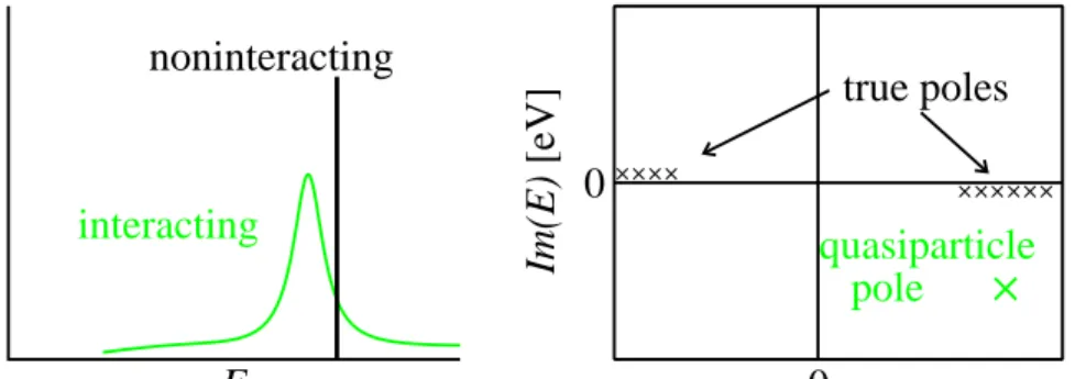
Figure 2.1: Left: schematic representation of a non-interacting and interact-ing spectral functionA(E) on the real energy axis. Right: the pole structure in the complex plane.

the entitity preferably used in theoretical studies to discuss the electronic structure because it does not depend on the experimental setup.

The connection to Green’s function theory is given by the Lehmann rep-resentation of the one-particle Green’s function

G(x,x′_{, ω}_{) =}X s fs(x)f∗ s(x′) ω₋Es±iη , (2.38)

where iη is an infinitesimal imaginary part. The positive (negative) sign applies for states above (below) the Fermi energy. The spectral function is then given by

A(x,x′_{, ω}_{) =} 1

πℑG(x,x

′_{, ω}₎_. _(2.39)

The poles of the Green’s function hence correspond to the one-particle addition and removal energies, also known as single-particle excitations. In an extended interacting system, the infinitely many excitations can merge into peak-like features that can be effectively described by a single pole (cf. Fig. 2.1). This pole has a finite imaginary part and describes the quasiparticle excitation. The real part of the quasiparticle energy corresponds to the peak maximum of the energy distribution when an electron is added or removed, for instance in an (inverse) photoemission experiment. The imaginary part determines the life-time broadening (peak width).

It must be emphasised that the concept of a quasiparticle is an inter-pretation of the experimentally observed many-body spectrum in terms of one-particle-like excitations. The quasiparticle concept is used for various types of excitations, for instance electron-hole pairs (excitons) or vibrations

(16)

(phonons). In the context of one-electron excitations, these quasiparticles can be viewed as a hole or an electron surrounded by its polarisation cloud. Quasiparticles have a finite lifetime due to dephasing, i.e., decay into other quasiparticles. because the true many-body eigenstates may contribute to more than one quasiparticle. In other words, a quasiparticle is not an eigen-state of the system but a superposition of eigeneigen-states. The actual formation and decay of an quasielectron in silicon has recently been followed in a time-resolved pump-probe experiment for the first time [54].

The connection between the Green’s function and the Hamiltonian can be schematically written as

G(ω) = [ω₋H]−1 _. _(2.40)

Here, H denotes the effective one-particle Hamiltonian, which implicitly contains the electron-electron interaction. It can be split into a pure non-interacting part H0 (in which we include the Hartree potential) and a

non-local, energy-dependent self-energy Σ, i.e.

H(x,x′_{, ω}_{) =}_H

0(x) + Σ(x,x′, ω). (2.41)

In analogy to Eq. 2.40, a non-interacting Green’s function is defined from

H0. The connection between the non-interacting and the interacting Green’s

function is given by the non-local, energy-dependent self-energy Σ and will be discussed in the next section. Before we come to this part, we briefly address the use of DFT.

A byproduct of the DFT-KS calculation are the eigenenergiesǫiand eigen-functionsφi of the Kohn-Sham HamiltonianHKS_{. Strictly speaking, they are}

no physical observables except for the energy of the highest (partially) occu-pied state which equals the chemical potential of the electrons in the system (Janak’s theorem [55]). However, we may use them as first approximations to the quasiparticle energies and functions. Correspondingly, a non-interacting DFT-KS Green’s function GKS _{can be defined in analogy to Eq. 2.38. Such}

an approach can indeed explain a number of qualitative features of the quasi-particle spectra, owing much to the fact that the true Hamiltonian and the Kohn-Sham Hamiltonian share the non-interacting part H0.

However, DFT-KS cannot explain all aspects of the quasiparticle band structure. In addition, the available approximate functionals introduce fur-ther errors. The most important failure is the underestimation of the quasi-particle band gap in the LDA by typically 50–100% [23, 56]. This is partially due to inherent deficiencies of the LDA such as the self-interaction, which pushes the occupied states up in energy. However, even the KS band gap

(17)

using the exact exchange-correlation potential would differ from the quasipar-ticle gap because the true xc functional exhibits a derivative discontinuity12

at integer particle numbers [57]. Nevertheless, it has been found that the LDA wavefunctions are reasonable approximations to the quasiparticle func-tions in many bulk systems [23, 58, 59]. We will come back to this point later when we discuss quasiparticle corrections.

2.3.2 Hedin’s equations and the

GW

_{approximation}

Hedin has shown that the problem of computing the interacting one-particle Green’s function can be cast into five coupled equations in the framework of many-body perturbation theory [60]. These equations involve the independent-particle and full Green’s functionG0 andG, the polarisationP, the bare and

screened interaction v and W, the self-energy Σ, and the so-called vertex function Γ. For simplicity, we use the notation 1 = x1t1 for every pair of

one spatial and one temporal variable. A+ _{indicates that the time argument}

has been increased by an infinitesimally small, positive amount. Hedin’s equations are: P(1,2) = ₋i Z d3d4G(1,3)G(4,1)Γ(3,2,4) (2.42) W(1,2) = v(1,2) + Z d3d4v(1,3)P(3,4)W(4,2) (2.43) Σ(1,2) = i Z d3d4G(1,3)W(4,1+)Γ(3,4,2) (2.44) Γ(1,2,3) = δ(1,2)δ(2,3) + Z d4d5d6d7 δΣ(1,2) δG(4,5)G(4,6)G(7,5)Γ(6,7,3) (2.45) G(1,2) = G0(1,2) + Z d3d4 G0(1,3)Σ(3,4)G(4,2) (2.46)

This set of coupled equations cannot be solved directly due to the presence of the functional derivative in the definition of the vertex function. However, it is amenable to physically meaningful approximations. We will describe the equations in more detail before coming to the most important approximation, the GW approximation.

We first note that Equations 2.43 and 2.46 have the same structure, known as a Dyson equation. It describes the redressing of independent-particle propagators by interactions with the system, which for the electrons is called self-energy. G0 and G correspond to the propagation of electrons or holes

in the system, whereas v and W can be interpreted as propagators for the

(18)

quantum particles of the electric field. Thus, the polarisation function plays the role of the self-energy for the electric field particles, changing the bare Coulomb interaction into the screened Coulomb interaction. Correspond-ingly, the equations for the interaction kernels Σ and P, Eq. 2.44 and 2.42, have the same structure. They contain two propagators connected to one point of the interaction kernel and are connected via the vertex function to the other point of the kernel. This vertex function is a three-point kernel that describes all possible ways how a (dressed) electron is scattered when a (screened) electric field particle is created or annihilated.

Approximating the vertex function by its first term, i.e. Γ =δδ, we arrive at the random phase approximation for the polarisation

P(1,2) =₋iG(1,2)G(2,1) (2.47) and theGW approximation for the self-energy

Σ(1,2) =iG(1,2)W(2,1+). (2.48) When the Dyson equation for the screened interaction is inverted, one obtains schematically

W−1₍₁_,_{2) =} _v−1₍₁_,₂₎₋_P₍₁_,₂₎_. _(2.49)

For the practical calculation, this equation is usually transformed13_.

Multi-plying from left and right with the square root14 _{of the Coulomb potential}

v1/2 _{and integrating yields the symmetrised dielectric function}

˜

ε(1,2) = δ(1,2)₋

Z

d3d4 v1/2(1,3)P(3,4)v1/2(4,2), (2.50)

from which the screened interaction can be computed via

W(1,2) =

Z

d3d4 v1/2(1,3)˜ε−1₍₃_,₄₎_v1/2₍₄_,₂₎_. _(2.51)

It must be emphasised that for a plane-wave basis, the integrations appear only formally sincev1/2 _{is diagonal in reciprocal space (see also Sec. 2.2.1).}

13_Since_v _and _W _{are singular in reciprocal space, the plane-wave representation of} _W is “ill conditioned”, i.e. the magnitude of the matrix elements varies strongly. This may lead to numerical inaccuracies or instabilities in the numerical inversion.

14_{The square root of a}_v₍₁_,_{2) is naturally defined by}

Z

d3 v1/2(1,3)v1/2(3,2) =v(1,2),

(19)

In practice, it is very common to employ further approximations. To solve 2.47 – 2.51, it would seem reasonable to iterate Eq. 2.46 and Eq. 2.47 – 2.51 to self-consistency. However, this is rarely done. Instead of using the full Green’s function G, the non-interacting Green’s function G0 is used

as a first approximation in Eq. 2.47 and Eq. 2.48. We use this approach, denoted G0W0, in all the actual calculations. The quality of this

approx-imation has been under debate over the last years. It proves to be very successful for describing the pole structure of the Green’s function in con-nection with pseudopotentials and Kohn-Sham DFT in the LDA or EXX as the independent-particle starting point [23, 56, 62]. Various flavours of self-consistency have been proposed. The conceptually simplest version is full self-consistency within the GW/RPA scheme, i.e., employing GGW from the Dyson equation (Equation 2.46) for the construction of the polarisabil-ity and the self-energy in the next iteration. This self-consistency scheme was applied for the homogeneous electron gas [63], closed-shell atoms [64], and silicon [65]. However, it was observed that the agreement with exper-iment for the quasiparticle spectrum does rather worsen than improve. It was suggested that this might be attributed to an inconsistent treatment of higher-order diagrams. Iterating the GW equations implicitly introduces higher-order diagrams in the Green’s function, which are believed to be can-celled to a large degree by the vertex [64]. In other words, the independent quasiparticle picture may be good for describing the single quasiparticle exci-tations of the system, it is worse for the two-particle random-phase polarisa-tion. This is in line with findings for the dielectric function computed in the RPA. Computing it from the Green’s function obtained from the G0W0

self-energy is usually not better than employing the non-interacting G0 from the

LDA [62]. Instead, explicit particle-hole interactions must be included, e.g. by the Bethe-Salpeter equation [62]. In approximate self-consistent schemes, the self-consistency is imposed only for the construction of Σ or for the quasi-particle energies [66–69]. Since these schemes give different results and the issue of self-consistency is still controversial, we do not go beyond theG0W0

approximation.

2.3.3 The quasiparticle equation

For the interpretation of PES or IPES in terms of single quasiparticle exci-tations, the quasiparticle poles of the Green’s function need to be identified. These are obtained as the zeroes of the inverse Green’s function, which is related to G0 via the the Dyson equation (2.46):

G−1₍_x_,_x′_{, ω}_{) =} _G−1

(20)

Since the non-interacting Green’s function is the inverse ofω₋H0, the

(right-hand) quasiparticle wavefunctions corresponding to the quasiparticle pole

ω=ǫqp _{are solutions to} −1 2∇ 2₊_V ext(x) +VH(x) φqp₍_x_{) +}Z _d_x′ _Σ(_x_,_x′_{, ǫ}qp₎_φqp₍_x′_{) =}_ǫqp_φqp₍_x₎_. (2.53) We note a few things here. Since the self-energy is not Hermitean, the left and right eigenfunctions for a given eigenvalue are different and the eigenvalues are in general complex. The left (or right) eigenfunctions do not form an orthogonal set. Furthermore, the quasiparticle energy ǫqp _{appears as the}

argument of the self-energy and on the right-hand side, i.e. the equation must be solved iteratively.

Eq. 2.53 is reminiscent of the single-particle equations from KS-DFT, the difference being that the local exchange-correlation potential has been re-placed by the non-local self-energy. To solve Eq. 2.53, the quasiparticle wave-functions φqp _{are expanded in terms of the KS wavefunctions} _φDFT

n , which

form a complete orthonormal basis set. By multiplying with (φDFT

n (x))∗ and

integrating over x, and then exploiting that the term in curly brackets of Eq. 2.53 can be written asHKS₋_V

xc, we arrive at the algebraic equation (in

Dirac notation) X n′ ǫnδnn′+hφDFT_n |Σ(ǫqp)−V_xc|φDFT_n′ i hφDFT_n′ |φqpi=ǫqphφDFT_n |φqpi, (2.54) where we have inserted 1 =P

n′|φDFT_n′ ihφDFT_n′ |.

In practice, the matrix of the operator Σ(ǫqp₎₋_V

xc is usually dominated

by the diagonal elements n = n′ _{[58, 59, 70], which we also found for the}

systems of this work. Neglecting the small non-diagonal elements yields the quasiparticle energy equation

ǫqp_n =ǫDFT_n +_hφDFT_n _|Σ(ǫqp_n )₋Vxc|φDFTn i, (2.55)

where the second term on the right hand side defines the quasiparticle correc-tion. This result corresponds to applying first-order perturbation theory for the perturbation Σ(ǫqp₎₋_V

xc (note the quasiparticle energy in the argument

of Σ). The quasiparticle correction still contains the quasiparticle energy, i.e., Eq. 2.55 must be solved iteratively.15

The derivation above does not require Vxc to be exact. The

“quasiparti-cle corrections” therefore comprise not only the self-energy (or quasiparti“quasiparti-cle)

15_{An alternative is to expand the energy-dependence of the self-energy matrix element} in a Taylor series aroundǫDFT

(21)

effects absent from the exact KS band structure, but also correct for defi-ciencies of the exchange-correlation functionals used in practice, notably the self-interaction. It is likely that both effects contribute significantly to the total correction, but in general, they cannot be disentangled easily. The term “quasiparticle correction”, though well established, should therefore be used with care.

When important physical effects are incorrectly described by the chosen density functional, large differences between the DFT-KS and the quasiparti-cle wavefunctions may arise. This is in particular the case for image states far away from the surface, where DFT-LDA yields a qualitatively wrong poten-tial [30, 71]. The transition from Eq. 2.53 to Eq.2.55 would then introduce significant errors. In such cases, the quasiparticle equation (Eq. 2.54) should be diagonalised. Whether such a diagonalisation is necessary or not can be decided by inspecting the magnitude of the off-diagonal elements of the per-turbation operator Σ₋Vxc. For all the GW calculations in this work, the

off-diagonal elements were therefore computed, too, and found to be negligi-ble in most cases. The diagonalisation may also be important for properties that depend on the quasiparticle wavefunctions. This has been highlighted for the reflectance anisotropy spectrum of GaAs(110) which changes signifi-cantly when one employs the quasiparticle wavefunctions rather than the KS wavefunctions although the error in the quasiparticle energies introduced by the perturbation approach is less than 0.1 eV [72].

2.3.4 GW

_{implementation: the space-time method}

The GW space-time method exploits the fact that many of the transforma-tions in a GW calculation can be efficiently performed in either real space and imaginary time or in reciprocal-space and imaginary frequency [73, 74]. The transformations between real space and reciprocal space can be effi-ciently computed with Fast Fourier Transforms, whereas the time-frequency Fourier transforms are performed via analytically enhanced Gauss-Legendre integrations [75].

An important practical aspect of the space-time approach is the separa-tion of theG0W0 self-energy into a static exchange

Σx(r,r′) =G0(r,r′,0+)v(r−r′) (2.56) expression ǫqp n = ǫDFTn + h φn|Σ(ǫDFTn )−Vxc|φni 1− ∂ω∂ hφn|Σ(ω)|φni _ω₌_ǫ_DFT n .

(22)

and a dynamic correlation part

Σc(r,r′, t) =G0(r,r′, t)(W0(r,r′, t)−v(r−r′)δ(t)). (2.57)

In the following, we employ the symbols G, P, ε, and W to denote the non-self-consistent Kohn-Sham Green’s function, polarisation, dielectric ma-trix, and screened interaction, respectively, in order to improve the read-ability. Except for the construction of the Green’s function, all formulae remain valid for the self-consistent case. If we assume a non-magnetic sys-tems for simplicity (the extension to a spin-dependent Green’s function is straight-forward), the computational steps to construct the self-energy ma-trix elements from the output of a preceding DFT calculation are:

1. Construction of the non-interacting Green’s function G in real space and imaginary time from the Kohn–Sham eigenfunctionsϕnkand eigen-values ǫnk (the Fermi level defines the energy zero)

G(r,r′_;_iτ_{) =}_i Ω (2π)3 Z BZd 3_k        occ P n ϕnk(r)ϕ ∗ nk(r′)e−ǫnkτ, τ <0, −unoccP n ϕnk(r)ϕ ∗ nk(r′)e−ǫnkτ, τ >0, (2.58) where Ω denotes the unit-cell volume and the integral overkruns over the first Brillouin zone,

2. formation of the irreducible polarisability P in the random-phase ap-proximation in real space and imaginary time

P(r,r′_;_iτ_{) =}₋₂_iG₍_r_,_r′_;_iτ₎_G₍_r′_,_r_;₋_iτ₎_, _(2.59)

3. Fourier transformation of P to reciprocal space

PGG′(k, iτ) = 1 Ω Z d3r Z d3r′ _P₍_r_,_r′_;_iτ_)e−i(k₊G₎_·r₊_i₍k₊G′₎_·r′ (2.60)

and to imaginary frequency,

4. construction of the symmetrised dielectric matrix in reciprocal space

˜

εGG′(k, iω) =δGG′ −

4π

|k+G_||k+G′_|PGG′(k, iω), (2.61)

5. inversion of the symmetrised dielectric matrix for eachk-point and each imaginary frequency,

(23)

6. subtraction of that part of the dielectric matrix that gives rise to the long-range interaction ˜ ε−1,sr GG′(k, iω) = ˜ε− 1 GG′(k, iω)− |k+G_|2 (k+G)T_L₍_iω₎₍_k₊_G₎δGG′ , (2.62)

where L(iω) denotes the macroscopic dielectric tensor, which is com-puted atk=0,

7. calculation of the short-range part of the screened Coulomb interaction in reciprocal space WGGsr ′(k, iω) = 4π |k+G_||k+G′_|ε˜ −1,sr GG′(k, iω), (2.63)

8. Fourier transformation of Wsr _{to imaginary time and to real space}

Wsr(r,r′_;_iτ_{) =} 1 (2π)3 Z BZd 3_k X G,G′ WGGsr ′(k, iτ)e i(k+G)·r₋i(k+G′₎_·r′ , (2.64) 9. construction of the long-range screening part Wlrs ₌ _Wlr₋_v _{in real}

space and imaginary time (see also Section 3.2.3),

10. construction of the screening part Ws ₌ _W ₋_v _{of the screened}

inter-action

Ws(r,r′_;_iτ_{) =}_Wsr₍_r_,_r′_;_iτ_{) +}_Wlrs₍_r_,_r′_;_iτ₎ _(2.65)

11. formation of the correlation self-energy in real space and imaginary time

Σc(r,r′;iτ) =iG(r,r′;iτ)Ws(r,r′;iτ), (2.66)

12. computation of the matrix elements of the correlation self-energy

hϕnk|Σc(iτ)|ϕnki= Z d3r Z d3r′_ϕ∗ nk(r)Σc(r,r′;iτ)ϕnk(r′), (2.67)

13. Fourier transformation of_hϕnk|Σc(iτ)|ϕnki to imaginary frequency. The matrix elements are then analytically continued to the real frequency axis by fitting a multi-pole function on the imaginary frequency axis [74]. The matrix element of the static exchange self-energy Σx=Gv are obtained

(24)

Equation 2.58, forming the exchange self energy analogous to Equation 2.66, and computing the matrix elements analogous to Equation 2.67. Finally, the quasiparticle energiesǫqp_nk are given by the solution of

ǫqp_nk=ǫnk+hϕnk|Σc(ǫqpnk) + Σx−Vxc|ϕnki, (2.68) where Vxc is the exchange-correlation potential used in the underlying DFT

calculation.

We note that we have improved the numerical implementation of the spa-ce-time method, notably the computation of the Green’s function (Eq. 2.58), the inversion of the dielectric matrices (Step 5), and the computation of the matrix elements (Eq. 2.67). While leaving the advantageous scaling be-haviour of the space-time method unchanged, the modifications greatly im-prove the numerical efficiency and reduce the overall run-time by a factor 3–5. Further modifications aimed at reducing the main memory and disk space requirements. These modifications are described in Appendix E and have been necessary to make the calculations in this thesis feasible.