Software-Based Ray Tracing for Mobile Devices

(1)

MATIAS KOSKELA

SOFTWARE-BASED RAY TRACING FOR MOBILE DEVICES

Master of Science thesis

Examiners: D.Sc. Pekka Jääskeläinen & Prof. Jarmo Takala

Examiners and topic approved by the Faculty Council of the Faculty of Computing and Electrical Engineering on 4th February 2015

(2)

i

ABSTRACT

MATIAS KOSKELA: Software-Based Ray Tracing for Mobile Devices Tampere University of Technology

Master of Science thesis, 51 pages August 2015

Master’s Degree Programme in Information Technology Major: Pervasive Systems

Examiners: D.Sc. Pekka Jääskeläinen & Prof. Jarmo Takala

Keywords: Ray Tracing, Bounding Volume Hierarchy, Compression, Half-Precision Floating-Point

Ray tracing is a way to produce realistic images of three dimensional virtual scenes. It scales more to the number of pixels in the image than to the amount of details in the scene. This makes it an interesting application for mobile systems, which in general have smaller screens.

Modern high-performance ray tracing depends on special acceleration data struc-tures such as bounding volume hierarchies. Compressing the size of the bounding volume hierarchy leads to smaller memory bandwidth usage. This should be espe-cially beneficial for mobile systems, which in general have smaller memory band-width. Compression also reduces cache misses and memory usage. Unfortunately, compression reduces the quality of the data structure, leading the ray traversal into unnecessary computations. In addition, compression increases the amount of work which needs to be carried out in the performance critical inner loop.

The previous work on bounding volume hierarchy compression concentrates on in-ferring some of the coordinates from other coordinates or using different integer precisions. This thesis concentrates on using half-precision floating-point numbers, which have potential due to their greater dynamic range. If the halfs are too inaccu-rate for use as plain world coordinates, they can be used with hierarchical encoding. This restores the quality of the data structure back to original, but it requires even more work in the inner loop.

Halfs reduce the whole memory usage by 7% and cache misses by 16%. Furthermore, they reduce power usage by 1.7%. The halfs’ effect on the performance is heavily dependent on the targeted hardware’s support for them. If decompression of the halfs is too slow, they will have a negative impact. Compared to integers, halfs have better performance in the so-called teapot-in-a-stadium problem.

(3)

ii

TIIVISTELMÄ

MATIAS KOSKELA: Ohjelmistopohjainen säteenjäljitys mobiililaitteille Tampereen teknillinen yliopisto

Diplomityö, 51 sivua Elokuu 2015

Tietotekniikan koulutusohjelma Pääaine: Pervasive Systems

Tarkastajat: TkT Pekka Jääskeläinen & prof. Jarmo Takala

Avainsanat: Säteenjäljitys, Rajaustilavuushierarkia, Pakkaus, 16-bittinen Liukuluku

Säteenjäljityksellä tuotetaan realistisia kuvia kolmiulotteisista virtuaalimaailmoista. Säteenjäljityksen nopeus riippu enemmän kuvan koosta, kuin virtuaalimaailman yk-sityiskohtien määrästä. Tämän takia se on kiinnostava vaihtoehto mobiilialustoilla, joilla yleisesti ottaen on käytössä pienemmät näytöt.

Tavallisesti säteenjäljitystä kiihdytetään erityisillä kiihdytysrakenteilla, kuten ra-jaustilavuushierarkialla. Rajaustilavuushierarkian tiedon tiivistäminen johtaa pie-nempään muistikaistan käyttöön, jonka pitäisi olla erityisen hyödyllistä yleisesti vähemmän muistikaistaa omaavilla mobiililaitteilla. Lisäksi tiivistäminen vähentää välimuistihuteja ja muistin käyttöä. Valitettavasti tiivistys huonontaa kiihdytysra-kenteen laatua, joka johtaa rakiihdytysra-kenteen turhaan läpikäyntiin. Se myöskin lisää työtä suorituskyvyn kannalta tärkeimmässä sisäsilmukassa.

Aikaisempi tutkimus rajaustilavuushierarkioiden tiivistämisessä rajoittuu arvojen päättelyyn toisista arvoista ja eri tarkkuisten kokonaislukujen käyttöön. Tässä työs-sä tarkastellaan 16-bittisten liukulukujen käyttöä, joka on kiinnostavaa suuremman dynaamisen alueen ansiosta. Jos 16-bittiset liukuluvut ovat liian epätarkkoja suo-raan maailman koordinaatteina, voidaan niitä käyttää hierarkisesti. Tämä palauttaa tarkkuuden alkuperäiselle tasolle, mutta lisää entisestään laskentaa sisäsilmukkaan. Säteenjäljittimessä kokonaismuistinkulutus vähenee 7% ja välimuistihudit vähenevät 16%, kun käytetään bittisiä liukulukuja. Lisäksi tehon kulutus pienenee 1,7%. 16-bittisten liukulukujen vaikutus säteenjäljityksen nopeuteen on erittäin riippuvainen laitteiston tuesta niille. Suorituskykyä ei voida parantaa, jos 16-bittisten liukulu-kujen purkaminen on liian hidasta. Kokonaislukuihin nähden liukuluvut toimivat paremmin, jos virtuaalimaailmassa on enemmän yksityiskohtia yksittäisellä alueel-la.

(4)

iii

PREFACE

This thesis was done as a part of the ray tracing research carried out in the Cus-tomized Parallel Computing (CPC) group at the Tampere University of Technology (TUT). Most of the research described in this thesis was carried out by the author. However, the use of half-precision floating-points in ray tracing was Timo Viitanen’s idea and he also did the practical measurements that are described in Section 6.3. The hierarchical encoding explained in Subsection 5.2.1 was pointed out by Ken Cameron.

All images of 3D worlds in this thesis are made using the author’s own ray tracer, unless mentioned otherwise. In addition, the 3D version of TUT-logo, used in exam-ple images, was made by the author, based on the original printed TUT-logo. Other models used in the example images were made by Martin Newell, Anat Grynberg, Greg Ward, Frank Meinl, Marko Dabrovic, Guedis Cardenas, Morgan McGuire and Stanford 3D Scanning Repository.

I would not have managed without the help and comments of my supervisors Pekka Jääskeläinen and Jarmo Takala. In addition, Timo Viitanen’s ray tracing and Heikki Kultala’s technical comments were very helpful. Furthermore, I would like to thank the entire CPC group for fruitful discussions and comments.

I would also like to thank Toimi Teelahti, Adrian Benfield and Ken Cameron for helping with grammatical corrections.

Finally, I would like to thank my wife for all her support. Without it, graduating from the university would have been impossible.

Tampere, 20.7.2015

(5)

iv

LIST OF FIGURES

2.1 The concepts of different ray tracing styles . . . 4

2.2 Samples of different ray tracing styles . . . 6

4.1 The scene and it partitioned with a grid . . . 16

4.2 The scene partitioned with a quadtree . . . 17

4.3 The scene partitioned with a k-d tree . . . 19

4.4 The scene partitioned with a BVH. . . 20

4.5 Visualization of a 3D BVH . . . 20

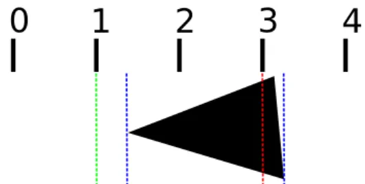
5.1 Quantization of triangle bounds . . . 34

5.2 Workloads for different precisions . . . 35

(8)

vii

LIST OF TABLES

6.1 The number of ray-AABB tests . . . 39

6.2 The number of ray-triangle tests . . . 39

6.3 The memory usages . . . 39

6.4 The total SAH costs . . . 40

6.5 The average power usages of different components . . . 41

(9)

viii

LIST OF ABBREVIATIONS

AABB Axis-Aligned Bounding Box ALU Arithmetic Logic Unit BIH Bounding Interval Hierarchy BVH Bounding Volume Hierarchy CPU Central Processing Unit

CUDA Compute Unified Device Architecture DLP Data-Level Parallelism

GPU Graphics Processing Unit

HLBVH Hierarchical Linear Bounding Volume Hierarchy ILP Instruction-Level Parallelism

k-d tree k-dimensional tree

LBVH Linear Bounding Volume Hierarchy LoD Level of Detail

MBVH Multi Bounding Volume Hierarchy nD n Dimensional

OpenCL Open Computing Language OpenMP Open Multi-Processing SAH Surface Area Heuristic

SBVH Split Bounding Volume Hierarchy SIMD Single Instruction, Multiple Data SIMT Single Instruction, Multiple Thread SoC System on a Chip

TLP Thread-Level Parallelism

(10)

1

1. INTRODUCTION

Images and videos produced by computer graphics are a crucial part of our lives today. They are used in several engineering applications, such as computer-aided design, simulation and promotion, as well as in entertainment including computer gaming, movie special effects and photo manipulation.

There are two main principles for drawingthree-dimensional (3D) computer graph-ics. The usual way is to rasterize 3D objects defined as a cluster of triangles. Rasterization of a triangle means setting the colors of those pixels that the trian-gle is contributing to. This method is sometimes called the conventional rendering pipeline. With the pipeline, rendering can be done quickly and in parallel. That is why it has been the most common way to draw 3D scenes. Additionally the major-ity of today’s graphics hardware is optimized for rasterization computation [PH11, Appendix A]. However there are effects, such as depth-of-field, reflection and refrac-tion, which are hard to achieve using the pipeline [AMHH08, Kos13]. Such effects are easily achieved with the other main 3D rendering method of tracing rays. In fact ray tracing is much closer to the way our eyes observe our surroundings. In a virtual 3D world, ray tracing simulates how photons would travel in the physical world. The main difference between rasterization and ray tracing is the data used in the main loop. Rasterization is done for each triangle and ray tracing is done for each pixel. In other words, rasterization calculates in front of which pixels each triangle is and ray tracing calculates which triangles are in front of each pixel. The problem with ray tracing is that it is not cost-effective with regards to compu-tation power. This is the reason for the ongoing search for algorithms, which would make ray tracing achieve real-time frame rates. There are already some frameworks, which claim to be fast enough [WWB∗14, PBD∗10, LSL∗13]. Unfortunately, they are not able to achieve the same frame rates and resolutions as the conventional ren-dering pipeline. In particular, the performance is lower with more realistic renren-dering results which are the main reason for using ray tracing.

The frame rate of ray tracing is more dependent on the numbers of pixels than the number of details in the scene. This makes it ideal for mobile devices, which in

(11)

1. Introduction 2 general have lower screen resolutions than laptop and desktop computers. Other characteristics of mobile devices are low power usage requirement and the smaller memory bandwidth. The low power usage requirement comes firstly from the fact that mobile devices run on battery power. The more power the system uses, the less time the battery lasts. Unfortunately, in the era of big displays and high-speed connections, the backlight of the display and the radio use most of the power and the other parts of the systems need to cope with what is left [CH10]. The other source for the low power requirement is that the mobile devices cannot overheat as much as desktop devices can, since it is hard for the user to use too hot handheld devices. Furthermore, active cooling of the device would require more power, which would make the battery die even faster.

One way to save power is to use low-precision data types. Both the storage of fewer bits and the computations using them can be done with lower power usage. This requires that the hardware has support for the data type. Unfortunately, compressed data is usually less accurate, which needs to be taken into account somehow. Either the user needs to bear with the lower quality or the data needs to be recovered to a level where it is indistinguishable from the original data.

This thesis focuses on optimizing ray tracing and in particular it describes what influences compressing the data structures have. This is expected to be especially beneficial on mobile systems, due to the smaller memory bandwidth.

The previous work in this field focuses on inferring numbers from other numbers or using fixed-point representation. This thesis compresses a commonly used data structure, the bounding volume hierarchy, using half-precision floating-point num-bers. Floating-point numbers are interesting compared to integers due to their greater dynamic range. Additionally, some mobile devices have native support for half-precision floating-point numbers and they can be better suited for floating-point calculations than integer calculations.

Sophisticated techniques to achieve complex light effects are left out of the thesis to keep it focused on the optimization and the compression. Nevertheless, the prin-ciples of different ray tracing algorithms are explained briefly in Chapter 2, which also describes implementation of a simple ray tracer. Common parallel hardware architectures used for accelerating ray tracing are described in Chapter 3. General optimization strategies, that can be applied to the most of the ray tracing applica-tions, are explained in Chapter 4. Chapter 5 describes how the bounding volume hierarchy can be compressed with half-precision floating-point numbers. Chapter 6 evaluates the proposed method and finally Chapter 7 concludes the thesis.

(12)

3

2. RAY TRACING

Ray tracing can be divided into four main categories: ray casting, Whitted-style ray tracing, distributed ray tracing and physically based rendering. These categories have different capabilities of producing complex effects. In general, more complex effects can be produced by using categories that shoot more rays. Fortunately, ray traversal can be optimized in a similar manner regardless of from which category the ray tracing algorithm is used.

2.1 Ray Casting

The idea of ray casting is to send one ray for each pixel from the camera. Each ray finds the closest intersection with the scene, which can be seen in Fig. 2.1(a). With this information, similar shading to conventional rasterization pipeline can be achieved. Ray casting is non-recursive ray tracing. It is a special sub-category of ray tracing in which only the first rays are traced from the camera, without any reflections or refractions [Bou05, p. 6].

Some volume rendering algorithms are also called ray casting. Those algorithms trace only the first rays from the camera, but they trace them through all of the geometry in the whole scene. This way they are able to find out all the intersections and calculate how much each volume affects the color of the pixel.

2.2 Whitted-Style Ray Tracing

In Whitted-style ray tracing, once the closest intersection is found, new secondary rays are sent to the directions of reflection and refraction [Whi79]. These directions need to be examined only if the properties of the material state so. Spawning new rays means that algorithm works recursively. The final color of the pixel is the weighted sum of all the rays. The weights are decided based on the material properties. For example, a perfect mirror material would only use the result of the ray sent from the mirror surface to the reflection direction.

(13)

2.3. Distributed Ray Tracing 4

casting rays camera

lamp

(a) ray casting

primary ray camera

shadow ray

secondary rays lamp

(b) Whitted-style ray tracing

primary ray camera

shadow rays

secondary rays lamp

(c) distributed ray tracing

gathering rays camera

lamp

shooting rays

(d) path tracing

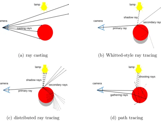
Figure 2.1 The concepts of different ray tracing styles. For visualization reasons only few rays are shown.

In addition to the reflection and the refraction rays, algorithms are usually using shadow rays. These are rays which are sent from the found intersect position to the light source to check if there are any objects between them. If there is anything between the position and the light source that means that the position is not affected by the light. These concepts are visualized in Fig. 2.1(b).

If the scene contains just a single point light, a typical Whitted-style ray tracer sends one to three new rays from the closest intersection point of each ray. This is continued recursively until the material of the intersected primitive states that it does not need any more extra rays or some kind of hard threshold for recursion depth is met. This threshold could be, for example, a limit in the recursion depth. Another example is a lower limit in the recursion ray’s weight.

2.3 Distributed Ray Tracing

Distributed ray tracing is an advanced version of Whitted-style ray tracing. The difference is that instead of just one reflection and one refraction secondary ray distributed ray tracing might sent more of them based on the material properties [CPC84]. This is visualized in Fig. 2.1(c) . The result of this is a more realistic image with effects, such as, soft shadows, fuzzy reflections, depth-of-field and motion blur.

(14)

2.4. Physically Based Rendering 5 Soft shadows can be achieved by sampling an area light using multiple shadow rays. The brightness of a point in the 3D scene is decided by how many of shadow rays are able to see the light. Soft transition on the shadow edges is achieved because in those areas some of the shadow rays are blocked by shadow casting objects and some are not.

Similarly to soft shadows, fuzzy reflections can be done by sending multiple sec-ondary rays to varied directions and calculating an average of them. Depth-of-field is a result of averaging multiple samples of primary rays from different origins. In contrast, motion blur is a result of averaging multiple samples in time.

2.4 Physically Based Rendering

The human eye measures the amount of photons coming from different directions. The paths of a single photon or a group of them can be easily simulated with rays. In general, physically based rendering tries to solve the so-calledrendering equation. The result of the equation is the total amount of light emitted in to the viewer’s direction from a point in 3D space [Kaj86]. This is calculated based on the incoming light and material properties.

There are many algorithms that try to solve the rendering equation. One of them is called path tracing. Path tracing software can use rays starting from each light source or rays starting from the camera. The third option is to use a combination of both of these approaches.

Shooting raysare sent from the light sources of the 3D world. Every time a shooting ray intersects something, it is randomly reflected or refracted. Instead of completely random directions, the distribution is weighted so that more rays are sent in the actual reflection direction. The distribution weights are decided based on the ma-terial properties. For example, a mirror mama-terial sends rays primarily towards the reflection direction. This is repeated until the ray intersects the imaginary cam-era or exits the scene area. Every time a ray finds the camcam-era it adds photons to the pixels. Based on the photons, the image starts slowly emerge. The more rays are traced, the better image quality is. Of course, there is one great problem with this technique; it takes a lot of computation time to produce even small images. As stated above the rays are going in random directions and, therefore, they are unlikely to find the camera.

The simplest way to optimize shooting rays is to reverse the ray direction. Instead of tracing rays from the lights, they are traced from the camera. It is more likely to find

(15)

2.4. Physically Based Rendering 6

(a) ray casting (b) Whitted-style ray tracing

(c) path tracing (rendered in hours) (d) path tracing (rendered in seconds)

Figure 2.2Samples of different ray tracing styles. Path tracing images were rendered with LuxRenderer [Lux15].

one of the many lights than to find the only camera. Additionally, the lights can even be area lights that cover areas instead of just one point. Intersection with an area is more likely than with a point. Rays starting from the camera are calledgathering rays, because they gather the information of what they intersect and set the color of pixel based on that. Just like the direction of the shooting ray, also gathering ray’s direction is decided based on material dependent weighted distribution. Examples of shooting rays and gathering rays can be seen in Fig. 2.1(d).

Path tracing can be made faster by combining the two basic path tracing approaches. For example inphoton mapping the shooting rays distribute light to the scene. Then gathering rays gather some of this distributed light. Finally, the color is decided based the gathered light. On the other hand, in bidirectional path tracing one gathering ray and one shooting ray are traced at the same time. After every found

(16)

2.5. A Basic Ray Caster 7 intersection, tests are performed to see if any of the gathering ray’s intersections can see any of the shooting ray’s intersections. If the rays can see each other, the amount of light which is going along the clear path can be calculated.

Examples of image quality of three ray tracing categories can be seen in Fig. 2.2. Ray caster’s (Fig. 2.2(a)) colors are only darker on the parts that are pointing away from the light and there are no shadows cast. For example, the inside of the dragon’s mouth should be in the shadow of the upper jaw. In Whitted-style ray tracing (Fig. 2.2(b)) there are shadows and reflections (it also supports transparent objects). These are possible because of the shadow rays and recursive secondary rays. There are two point lights in the scene. This can be observed from the two hard shadows on the floor under the teapot. The maximum recursion count in this example was one, which can be seen in the spout’s reflection on the teapot which is not reflecting like the actual spout is. In addition to basic recursive ray effects, path tracing (Fig. 2.2(c)) supports caustics and soft shadows which make the image much more realistic. A caustic effect can be seen under the orange glass TUT-logo where there are some brighter areas. An example of the soft shadows can be seen on the wall next to the white box. In the other path tracing image (Fig. 2.2(d)) the result of tracing only the first rays can be seen. In the image there are bright spots which are results of the ray randomly finding the light very quickly. After many more rays the actual color emerges.

2.5 A Basic Ray Caster

In this section a basic ray casting algorithm is demonstrated. The basic ray casting software is straightforward to implement. First, the software needs some kind of ray-object intersection test. The objects of the 3D scene are either loaded from a file or procedurally generated. Then, one ray is sent from every pixel. Each ray is tested against every object with the intersection test, and the color is chosen based on the material at the closest intersection point. Naturally, it is important that the intersection tests are as optimized as possible because the software is going to have to compute an enormous number of them.

A ray-object test can be any kind of 3D ray intersection test, but whatever kind of test is selected it will limit the kind of objects that can exist in the 3D world. For example, if the test is a ray-ball test, there can be only balls in the scene. Of course there can be several different tests in the software to enable support for multiple object types. The most common test is the ray-triangle test, because 3D object design tools usually save their objects as triangles.

(17)

2.5. A Basic Ray Caster 8 3D objects are designed using design software which saves the resulting triangles to a file. At the start of the execution, the ray casting software reads the file and stores the objects in its memory. Another way to do this is to procedurally generate objects, but it is hard work to achieve interesting and detailed objects this way. While procedural generation often requires complicated math, most design tools can be used intuitively by artistic people. After the objects have been loaded, the software initializes the rays.

The ray casting starts by deciding the directions in which the primary rays are to be sent. Usually they start from one point which is designated as the imaginary camera. The direction of each is set based on the pixel that the ray is contributing to. The directions of the rays contributing to the upper half of the image are turned upwards and those contributing to the lower half are turned downwards. The further the pixel is from the center of the image the more the ray is turned. The same idea is used for the right and left halves of the image. The maximum turn angle is in accordance with the simulated focal length of the camera. The greater the maximum angle, the more of a fish-eye effect there is in the resulting image. A smaller maximum angle replicates a greater zoom on the camera lens. Once the direction has been decided the rays need to be traced.

Tracing means finding the intersection points of the ray with the objects in the 3D world. It might be the case that all of the intersections are required, or that only the closest intersection is needed, or even only the knowledge of whether the ray intersects anything at all. For example, in basic ray casting only the closest intersection is needed, and the color is decided based on the material of the closest object. The most obvious way to find the closest intersection is to test the ray against each object in the 3D world. However, with bigger worlds this is impractical to compute.

If only the closest intersection is wanted, it might seem a good idea to sort all the objects based on their distance from the camera and then to test them in order, from the closest to the farthest. Unfortunately, this sorting is still too computationally heavy, because the camera might move and turn between the frames, so the sorting needs to be done all over again. In addition, if the ray does not intersect anything, the software is still testing for intersections with every object. That is why special data structures are used for ray tracing. These structures divide the 3D space into smaller sections. In this way, the rays can avoid doing the intersection test with an object that is far from the ray. The most common of these structures are introduced in Section 4.1. Nevertheless, before optimizing the ray tracing code it is important to know common hardware architectures which execute it.

(18)

9

3. COMMON COMPUTER ARCHITECTURES

FOR PARALLEL COMPUTING

Before reaching the so-called power wall, faster processing was done by increasing the clock rate of a processor [PH11, p. 39]. The power wall means that increasing the clock rate increases the power usage and temperature too much. Notably a higher clock rate requires more voltage and power is proportional to the voltage squared.

In order to work around the power wall, different ways of parallel execution have become more common ways of speeding up processing. In general, parallelism can be divided into three main categories: Thread-Level Parallelism (TLP), Data-Level Parallelism (DLP) and Instruction-Level Parallelism (ILP). This chapter describes these different parallel computation architectures. They can be used singly or com-bined to accelerate ray tracing. Chapter 4 presents how some of these accelerations are done.

3.1 Thread-Level Parallelism

A thread is a part of software executing on its own and having its own program counter. The difference between a process and a thread is that the process has its own memory address space, while many threads share the same. Furthermore, a thread can be thought to be a path of execution within a process and there can be multiple threads in a process. Multiple threads can be used for dividing the work of a single process to multiple processors on amultiprocessor or for so-called hardware multithreading on a single processor.

The multiprocessor is a chip which has multiple processing cores, which can run multiple threads in parallel. The only connection between the threads is the memory that is shared between the processors. There can be so-called critical areas of execution in a software, which require that the data in the common memory is not read or written by any other thread while the critical area is executed. For handling these areas processors have special techniques such as locks. A Lock can be checked

(19)

3.2. Data-Level Parallelism 10 in one cycle and, if it is free, it is given to the checker. If the lock was not free, the checker will wait and check the lock again after some time. When the thread is leaving the critical area it needs to free the lock so that others can access the area. If locks are not handled correctly, it is possible to achieve a so-called deadlock. In deadlock a thread is waiting forever for a lock that is never going to be freed. Usually this causes the program to eventually freeze.

Hardware multithreading means that many threads share the functional units of a single processor [PH11, p. 645–648]. The main advantage of using multiple threads on a single processor is that they can hide costly stalls. Stalls occur when something is blocking the process from continuing the execution. For example, the process is waiting for data to be fetched from memory or it is waiting for a user input. The hardware can in that case change to a different thread automatically, which is called coarse-grained multithreading. The other option is that the hardware is changing threads all the time and skipping threads which are currently stalling. This can be called fine-grained multithreading if the hardware is changing the thread on every cycle or simultaneous multithreading if resources are dynamically scheduled to the threads which need them. Modern desktop processors utilize simultaneous multithreading.

Multithreading processors have the same programming challenges as multiproces-sors. Both multiprocessors and hardware multithreading are commonly used in modern Central Processing Units (CPU) and Graphics Processing Units (GPU), including mobile CPUs and GPUs.

3.2 Data-Level Parallelism

Single Instruction, Multiple Data (SIMD) is an example of data level parallelism. Additionally,Single Instruction, Multiple Thread (SIMT) is another example of data level parallelism, but it also resembles thread level parallelism.

3.2.1 Single Instruction, Multiple Data

SIMD means that a single instruction performs the same operation for multiple pieces of data. This can be thought to be the same as piecewise vector computa-tions. For that reason SIMD instructions are also commonly referenced as vector instructions. Contemporary desktop processor hardware supports 256-bit SIMD operations. This can be divided into, for example, eight 32-bit floating point calcu-lations or four 64-bit calcucalcu-lations. In addition, not all of the bits need to be used,

(20)

3.2. Data-Level Parallelism 11 which means that narrower vectors can be computed. The current trend is that new generations of SIMD extensions double the amount of bits each instruction can compute simultaneously.

Basically, a programmer can order the processor to fetch, for example, four numbers from memory and perform the same computation for all of them with a single instruction. This will lead to almost four times the speed, although loading four times as much data could slow it down. Even if the hardware has a capability for fetching all of the vector data at once, all of the data needs to be there in time. If a piece of the data is missing, all of the pieces have to wait for it to be loaded from slower levels of caches. Usually, the miss of some data can be avoided with proper data layout for the cache lines. If the computations are done one by one, other pieces of the data can be loaded while the first pieces are computed. Nevertheless, the computation itself is around four times faster than with a scalar processing unit performing same computations on four pieces of data.

With SIMD instructions the data streams are synchronized, which means that there is no need for complicated concurrence handling such as locks. The downside is that it can be impossible for some algorithms to have the type of data parallelism which allows them to be computed with vector instructions.

In addition to speed improvements, SIMD advantages include reduced program memory size, reduced need for control logic and reduced need for checking so-called hazards (both data and control) [PH11, p. 648–653]. With SIMD there is no need to store and fetch the same program multiple times for each piece of data, which saves power significantly. Additionally, the same control logic can control multiple Arithmetic Logic Units (ALU), because they are all doing the same work just for different data.

SIMD is commonly used in all kinds of CPUs and in GPUs including mobile devices. In addition, some GPUs use the SIMT execution model, which can include SIMD instructions.

3.2.2 Single Instruction, Multiple Thread

The difference between SIMT and SIMD is that SIMT applies the same instruction to multiple threads as well as to multiple pieces of data [LNOM08]. In SIMT, a group of threads, a so-calledwarp, is executed all at once in a SIMD like execution unit. Each single thread can even execute SIMD instructions, but depending on the hardware, this might reduce the warp size.

(21)

3.2. Data-Level Parallelism 12 The downside of SIMT is that if there is any branch divergence in the program the execution can handle only one branch at the time. This is done by running all of the commands in all of the branches to all of the threads, but masking out those that should not actually execute the branch. If there is a single if – else statement with equally long execution paths on both branches (and at least one thread takes the other branch than the other threads), only 50% of the benefits are achieved [PH11, p. A-29]. This means that heavily branching code likely runs faster on a scalar processor than a SIMT processor.

Some of the divergence could be avoided by reordering the warps so that as many warps as possible contain only threads that are executing the same branch or similar code. The easiest way to achieve this is if the programmer can reorder the data so that the ones that take the same branch are sent to the same warp. Otherwise, especially for small branches this might be too complicated for the hardware to manage.

This kind of execution model is especially beneficial for applications where the same small program, without much branch divergence, is executed for many different pieces of data. Examples of these kind of programs are graphics programs in other words the shaders, which do the same computations for every primitive vertex or pixel. The difference between each primitive vertex and each pixel is that their data is different and, therefore, the same small program needs to be run for every one of them individually. This is the reason why many desktop GPUs and some mobile GPUs utilize the SIMT execution model.

A common SIMT architecture has long latencies for each instruction [PH11, p. A-29–A-30]. The latency can be hidden by using hardware multithreading (described in Section 3.1). This means that there can be even more threads running in parallel. Today’s SIMT-based GPUs can theoretically have thousands of active threads run-ning in parallel. The amount of actual threads compared to theoretical threads is calledthread occupancy. In contrast, modern CPUs can have tens of active threads, but these threads are much more independent from each other than the threads on a GPU.

SIMT has same hardware level advantages as SIMD. On the software level, the difference to SIMD is that the programmer does not need to manually define the data parallel parts of the code. The code can be written in the scalar way for a single piece of data and the SIMT driver and hardware can decide the data parallelism dynamically. This way even if the hardware changes, thread occupancy can be kept high with the same code. The difference to conventional multithreading on a CPU

(22)

3.3. Instruction-Level Parallelism 13 is that all of the threads in a warp are running the same code. In contrast, with regular multithreading each thread might as well be running a totally different piece of the code.

3.3 Instruction-Level Parallelism

In Instruction-Level Parallelism (ILP) the hardware is actually running multiple instructions at the same time, even if it is abstracted in a way so that the programmer and the compiler can think that the hardware is running sequential code [PH11, p. 41]. This can be done, for example by sending instructions to apipeline so that the computation of the next instruction starts before the computation of the previous one ends. Another idea is to have multiple hardware units for different tasks and have a control logic, which realizes that some of the instructions can be executed in parallel, which is calledSuperscalar execution.

There are ways to make ILP utilization easier for the hardware. One is to unroll loops so that there are more sequential instructions modifying different data, but this usually requires more registers. In the author’s experience, ray tracing is somewhat register bound. Therefore, unrolling is probably not a good idea. Furthermore, it is the compiler’s job to do the unrolling, if it realizes that the loop is a good candidate for it.

3.4 Mobile Device Hardware Architecture

Mobile devices use all of the parallel computing architectures described in this chapter, but usually their resources are more limited compared to desktops. One notable characteristic of mobile device architectures is the reduced memory band-width, which reduces the power consumption. For this reason, algorithms for mobile devices are designed so that they use less memory bandwidth [AMS08].

A modern trend is that mobile devices have a so-calledSystem on a Chip (SoC). A SoC is a piece of hardware that contains multiple different kind of hardware units, which all are dedicated to their own tasks. For example, there could be a processor just for signal processing and a separate processor just for manipulating images from the device’s camera. SoCs use less power by shutting down some parts of the chip [EBA∗11]. In a way, SoC is a high level parallel computing architecture, because the hardware units can work simultaneously on their own tasks.

In the future, it is possible that the SoC contains a hardware unit dedicated to ray tracing. Either the ray tracing unit could be a part of the GPU, capable of drawing

(23)

3.4. Mobile Device Hardware Architecture 14 triangles with the conventional pipeline, or it could be a completely separate graphics processor. The advantage of the first approach is that the same resources could be reused, but it also sets many requirements for the unit. There is already a large body of work on this area [LSL∗13, SWW∗04, WSS05].

(24)

15

4. GENERAL RAY TRACING OPTIMIZATION

ALGORITHMS

In this chapter, the most common generic optimization algorithms for ray tracing are introduced. These are algorithms which can be used with many kinds of ray tracers on different kind of platforms.

Algorithms can be divided into two categories: online and offline optimizations. Offline optimizations are done before the actual tracing of the rays start and online optimizations try to optimize the code that is doing the tracing. Space partitions are ways of doing offline optimization. They are sometimes done again for every frame, but they are still done before the tracing. Online optimizations include parallel computing and optimizing the inner loop.

4.1 Space Partition

The most important optimization for ray tracing is data structure optimization. In this process, the 3D space is usually divided into smaller volumes. These vol-umes are usually stored in a tree-like structure. The space can also be divided into equally sized portions and stored in 3D array as in grid space partition. By using these principles, the ray traversal can be terminated as soon as possible. All of the most common space partition methods for ray tracinggrids,k-dimensional trees (k-d trees) and Bounding Volume Hierarchies (BVH) are described in this section [WMG∗09].

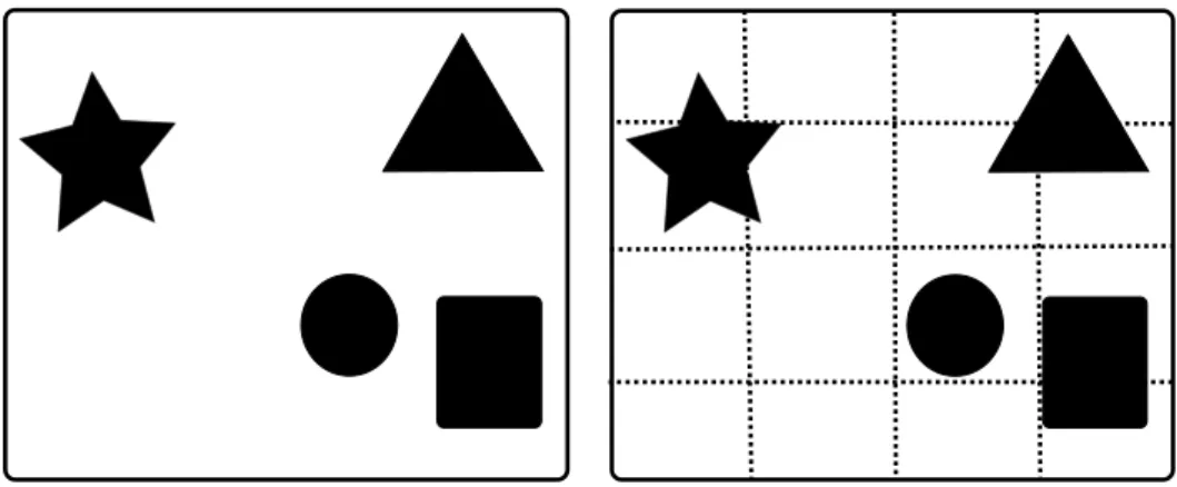
Space partition algorithms are demonstrated in the scene illustrated in Fig. 4.1. In the figure, the primitives are represented by different shapes, but all of them could as well be triangles. If one would like to make a ray tracer that would work with, for instance, star shaped primitives, they would need to either split the star into easier shapes like triangles or just implement a test which tells if a ray intersects the star or not. The figures presented in this section might not be the optimal solutions for each space partition algorithm in the example scene. They try to visualize how the algorithms work. All the algorithms work in 3D space, but due to the author’s

(25)

4.1. Space Partition 16

Figure 4.1 Left: Scene used for demonstrating the space partition algorithms. Right: A grid partitions the space into equally sized boxes. Notice that memory is used for the empty lower left corner and many primitives occupy more than one grid box.

rather limited drawing skills, every algorithm’s 2D equivalent is used in the figures.

4.1.1 Grids

Grids divide the space into equally sized boxes, which can be easily stored in a 3D array. The advantage of this is that if a ray’s starting position is in the middle of the scene, examination can start from the grid’s box corresponding to that position. This only requires a conversion function between the world coordinates and the 3D array coordinates. In addition, it is fast to find out which grid boxes a ray is going to intersect and traverse them in closest first order. The 2D space partitioned into a 2D array is illustrated in Fig. 4.1.

Traversing is done by first loading the grid box in which the ray starts and checking if the ray intersects primitives in it. Then traversing continues by taking the closest grid box which the ray is intersecting and is not yet examined. This is done over and over again as long as an intersection is found or the ray goes out of the scene. If there are multiple primitives in a box, and the ray is intersecting more than one of them, the result is the primitive with the closest intersection.

Disadvantages of the grids are handling big primitives and handling empty space. Big primitives are spread out to multiple grid boxes. This means that they need to be referenced in all of them. During traversal, the same primitive must be tested multiple times, even if it was already tested (and realised that the ray does not intersect with it). This can be avoided by adding a buffer of last tested primitives, but even with a quite small buffer, checking it becomes slower than just testing the primitive again. If there is an empty area in the scene, the grid is using memory

(26)

4.1. Space Partition 17 to store empty nodes. In the worst case this means that there are only a couple of nodes storing all the primitives (consider a case of two detailed models far apart from each other). In this kind of worst case scenario, using the grid might even be almost as bad as testing the ray intersection against every single primitive.

4.1.2 Octrees

Instead of storing data in equally sized grid boxes, data can be stored in a tree struc-ture. This way some of the branches can terminate earlier and shallower branches can be applied to empty areas of the scene.

While traversing the tree structure, at the root level, the ray is first tested to see if it can intersect with anything at all. If not, the traversal can terminate straight away. If the traversal indicates that the ray intersects a node in the tree, a similar test is performed for all the child nodes of the node. This is continued until all the branches have terminated, or reached the leaf level. At the leaf level, primitive intersection tests are performed to find out if the ray actually intersects any primitives in the leaf. This can be optimized by going through nodes in a depth first order and starting from the branch that contains the closest node to the ray origin and continuing to branches further away in the ray’s direction. In this way, the whole traversal can terminate as soon as an intersection is found.

An octree is one way to store the space into a tree structure [Mea82]. The idea of the octree is to split the space recursively into eight equally sized partitions. The recursion is terminated if there are no primitives at the branch at all. This way, memory is used for areas that actually need them. The octrees do not need to store the split position into memory, because they are always going to be in the middle

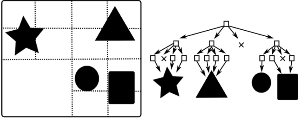
Figure 4.2Octree’s 2D equivalent quadtree partitions the space recursively into four equally sized boxes.

(27)

4.1. Space Partition 18 of the inner node. The inner node just needs to store eight pointers, which can be pointing to child branches, child leaves or null (empty node).

The example scene is partitioned using octree’s 2D equivalent quadtree in Fig. 4.2. The optimal quadtree would have been one where recursion had been stopped after the first split but it was continued in this example for demonstration purposes. Nevertheless, if the primitives are not equally sized and they are not laid out to fixed coordinate values, the octree nodes are not tightly bounded around their geometry. This means that there is empty space in the leaf nodes and that the same primitives are referenced in multiple leafs. Given these points the disadvantage of octrees is their rigidity. As mentioned in Subsection 4.1.1, referencing a primitive in multiple leaves forces traversal to test the same primitive multiple times. In contrast, empty space forces the traversal examine a leaf node, even the ray is actually far away from the node’s geometry. For these reasons octrees are not that commonly used in ray tracing.

4.1.3 K-Dimensional Trees

In k-d trees, like octrees, the division is always made along axes, but unlike octrees the space is split, not divided into 8 pieces [WH06]. Additionally, the position of the split can be freely chosen within the parent volume as long as it is along one of the three axes. In other words, in the k-d tree the space is split recursively into two parts which can be different sized. In k-d trees if a primitive is in the area of two leaves, it needs to be referenced by both of them, but because of the freely chosen split position most of these cases can be avoided. The freely chosen split position also allows tightly bound boxes around the primitives.

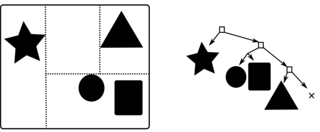
One way of partitioning our example scene using a k-d tree is shown in Fig. 4.3. Notice how in the example scene getting rid of empty space next to the triangle requires an empty node. Empty nodes might seem like a good idea because they are terminating immediately and do not require memory, but they might be bad for performance when using the parallel traversal techniques discussed in Section 4.2. K-d trees have been popular data structures for ray tracing for some time. In k-d trees, the nok-de only neek-ds to store two bits for the 3D axis ank-d one floating point number for the split position. In addition, k-d trees are also fast to traverse. Unfortunately, k-d trees are still quite rigid. For example, it is difficult to split the world into more than two parts, which is required by some parallel traversal techniques. Furthermore, it is difficult to adapt k-d trees for animated scenes. This usually requires building the whole k-d tree from scratch after every change in the

(28)

Figure 4.3 The k-d tree splits the space recursively into two different sized halves. Notice how getting rid of the empty areas around primitives requires more splits.

model [WIP08]. Therefore, more flexible data structures, like bounding volume hierarchies have been developed.

4.1.4 Bounding Volume Hierarchies

The idea of a BVH is to store the hierarchical structure of bounding volumes [KK86]. Usually these are Axis-Aligned Bounding Boxes (AABB), but spheres and other shapes can also be used. AABBs are boxes whose bounds are aligned to main axes of the scene. Compared to boxes with other orientations, intersection computations are faster using AABBs.

In BVHs, instead of just splitting the volume, smaller AABBs are taken from it. These smaller child AABBs can be positioned anywhere inside their parent. Using this approach, the child volumes are easily fitted so that no extra volume is left in them. When using k-d trees this process would require multiple splits. For this reason, some k-d tree algorithms utilize empty nodes [WH06]. Empty nodes are not as effective as the fitting achieved in BVHs. Because of the basic idea of the BVH, it is some times categorised as an object partition algorithm instead of the space partition algorithm.

An example of 2D BVH can be seen in Fig. 4.4 and visualization of 3D BVH for much more complex scene can be seen in Fig. 4.5. This kind of visualization can easily be made by setting a ray tracer to count how many intersection tests it does for each pixel to find the closest intersection with the primitives. Then the count of intersection tests is used to set the color of the pixel. In this example the pixel color was set to white and then darkened for each test the pixel had to make. When using BVH, each node needs to store six values, which correspond to the

(29)

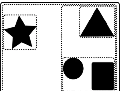
Figure 4.4 BVH fits tight axis-aligned bounding boxes around groups of primitives and produces a hierarchy of them.

minimum and maximum values of the AABB on every axis. Unfortunately, this requires more memory in the inner nodes than in the inner nodes of a k-d tree. Nevertheless, the k-d tree might require more memory in total, because it might be referencing to the same triangles so many times in the leaf nodes. There are ways to reduce the memory requirement of BVH inner node at the cost of extra computations. These ways are described in Section 4.4. To find out if a ray intersects the AABB of a BVH node, there needs to be a ray-AABB intersection test. The test requires some computation, even if it is as optimized as possible [AMHH08, p. 744] [PH10, p. 193].

Usually every triangle is stored in only one leaf of the BVH. This can be done because it does not matter if the child nodes are overlapping each other on any level. The advantage is that each primitive is tested only once. The disadvantage

Figure 4.53D BVH visualized by displaying the amount of work each pixel has to perform to find the closest intersection with the dragon model. The darker color means more work.

(30)

4.1. Space Partition 21 is that when the first intersection is found, it is possible that the traversal cannot terminate. Given that there might be a closer triangle in another overlapping branch even though the branches are travelled in closest first order. Some of the overhead can be reduced withSplit Bounding Volume Hierarchy SBVH, which tries to avoid overlapped sibling AABBs [SFD09]. The result is tighter fitted AABBs, but this requires references to the same primitive from multiple leaf nodes.

Despite the fact that BVH requires more computation and extra memory, it is very adaptable. The minimum and maximum values of the AABB of BVH nodes can be changed without rebuilding the entire data structure. Changing the values is required, for example, if there are animated objects in the 3D world. Of course, the quality of the tree decreases when values are changed from the optimal ones. For this reason, some ray tracers using BVHs update the values regularly and rebuild the tree only when the quality has decreased under a certain threshold. This way, both adaptability and good quality can be achieved.

4.1.5 Tree Construction with the Surface Area Heuristic

To generate high quality k-d trees and BVHs automatically, there needs to be a way of computing the quality of a single split. The Surface Area Heuristic (SAH) estimates how much work a ray tracer must do for a random ray to find out which triangles it intersects with in a given volume [MB90]. The basic equation of SAH can be as simple as

C =Sa×N ×T (4.1)

whereC is the cost of the finding the closest triangle, Sa is the surface area of the volume in which the tests are done, N is the number of triangles in the volume and T is the cost of a single triangle intersection test. In order to make ray tracing faster, the space can be divided into smaller volumes. The size of the volumes can be decided based on the SAH cost.

The division into smaller volumes begins with the whole space. All the possible split points are tested for the SAH cost of both possible child roots. The possible split points are the ones where any of the primitives start or end, because the optimal split is always one of these points. After all the possible split points are tested, the position with the lowest combined cost for both child volumes is chosen as the actual split position. Both child volumes can then be divided with the same algorithm, and the splitting can continue to their children in a recursive manner. The result of

(31)

4.1. Space Partition 22 this splitting is a tree-like structure which contains the so-called inner nodes, where space is divided, and the so-called leaf nodes, where primitives are stored.

Due to the idea of SAH, it is also easy to determine when to stop splitting and leave a volume whole. The cost if a node is left as a leaf has already been calculated in the parent level SAH test. For the split to be made, the sum of the costs of the two child nodes should be less than the cost of not splitting the node. The final parameter needed for this test is the cost of a ray tracing tree branch traversal step S. The equation for choosing whether to split a node is defined as

Cleaf < S+C1+C2 (4.2)

whereCleaf is the cost if this node is made into leaf,C1 the cost of the first child in the lowest combined total child cost andC2 is cost of the second child in the lowest combined total child cost. The node is made into a leaf and the recursion is stopped if Eqn. (4.2) is true. In that case, the SAH cost of the leaf is lower than the SAH cost of two children.

There are difficulties with this approach, though, because both the children are calculated as if they were leaves. However, the first children after the root are often the roots of deep sub-trees. In the case of a sub-tree, the cost estimate is not the same as the actual cost of the final node. Calculating the actual cost in the construction phase would be too computationally expensive, because for each possible split on every level it would require recursive calculation up to the leaf nodes.

SAH tree construction is used as the golden standard in most of the research ex-amining other construction methods. Usually these other methods try to make the construction somehow faster, because the SAH method is so computationally heavy.

4.1.6 Faster Tree Construction

There are many ways to speed up tree construction [Wal07]. For example, some parts of the tree can be built with faster methods that are based on a so-called Z-curve. The idea of the Z-curve is to give every position in 3D space an alternative single dimension coordinate. This coordinate is decided in a way so that objects close to each other in the 3D world also tend to be close in the Z-curve coordinate. If the whole tree is built using Z-curve without any SAH it is calledLinear Bounding Volume Hierarchy (LBVH) [LGS∗09] and if it is a combination of both methods, it is calledHierarchical Linear Bounding Volume Hierarchy (HLBVH) [PL10].

(32)

4.2. Ray Traversal Optimization 23 Another idea is to calculate the SAH values only for some points in the space, which is calledBinned SAH [DPS10]. For example, it is possible to test only eight points inside the parent AABB. The best of these points is then used instead of the actual best SAH position. Parent AABBs can be divided equally based on the volume or, if the primitives are already sorted, the points can be chosen so that each bin contains as many of the primitives.

While implementing his own ray tracer the author tried improving binned SAH by applying parabola fitting to the values found for bins. The idea was that the lowest point of the parabola is closer to the actual best SAH position than best bin. This seemed good, because in the example figures of SAH costs the values form nice clean parabolas. In reality the SAH cost curve can be very complex, to the point that the parabola found by curve fitting was upside down. This meant that the fitted parabola disagreed wildly with the actual best SAH position. Even with dirty hacks for caching problematic cases, parabola fitting gave only minor or not at all improvements on the original binned SAH. A similar idea was introduced by Hunt et al.[HMS06], but their approach took more samples in the problematic areas without any curve fitting. They claim that the approach achieves some performance increase.

4.2 Ray Traversal Optimization

This section describes online optimizations which are the optimizations that are used during the ray traversal. These optimizations can be done on a general level. However, for efficient implementation they require as much knowledge of the targeted hardware as possible.

4.2.1 Inner Loop

The inner loop is the part of the ray tracer which is looped over and over again in the ray traversal phase. It includes both the data structure traversal and the primitive ray test. Optimizing the inner loop means reducing the total latency of it to the minimum. Reduction can be done by pre-calculating values which are going to be the same on every loop iteration and by avoiding unnecessary branching in the loop. Usually the compiler should do this type of optimization, but if the code is complex, it might be too hard for it to detect that the optimization is possible. One typical optimization is to calculate a piecewise vector value inversion of ray direction before the inner loop, replacing a costly piecewise division in the ray-AABB intersection test with a relatively fast piecewise multiplication.

(33)

4.2. Ray Traversal Optimization 24 There are some frameworks which can be used for writing and compiling efficient parallel inner loops quickly. Examples of these frameworks areCompute Unified De-vice Architecture (CUDA),Open Computing Language (OpenCL) and Open Multi-Processing (OpenMP). The idea is that they can use special instructions and op-timize parameters based on the targeted hardware, which cannot be done with conventional C++ compiler. The advantages of these frameworks also include that the same code can be used for multiple platforms.

However, if the absolute optimal result for the targeted hardware is desired, it can be achieved by modifying or writing the inner loop using intrinsics or assembly language. Usually, this is quite slow work and the result is not portable to hardware using different instruction sets. On the other hand, the programmers can handle all of the resources themselves. This means that the resulting software can have better utilization of all resources than with the compiler deciding the utilization.

4.2.2 Packet Tracing

The idea of packet tracing is to trace more than one ray at a time. Using SIMD (described in Section 3.2.1), this is relatively simple. Instead of one ray’s origin and direction, the software loads groups of them and performs all of the same calculations for each one in the group in parallel [WGBK07].

But of course, there are some drawbacks. It is possible that only one ray requires further inspection of a space partition structure in which case an unnecessary in-spection is carried out on all of the rays. If it is assumed that the hardware actually has the same width SIMD instructions as the vector width of the software, even in the worst case the computation should not be slower than when tracing each ray one by one. However, if the hardware is emulating wider SIMD instructions by running the code with narrower SIMD instructions multiple times, packet tracing might slow down the software.

The advantages of packet tracing are decreased if the rays are not coherent. Co-herence means that the rays are going in almost the same direction. CoCo-herence is high when the primary rays are sent from the camera, but with the reflected and refracted secondary rays the coherence is much lower. Notably, the coherence of shadow rays can be somewhat high even after many recursion steps, because they are all going to the same light source.

Another problem with packet tracing is the fact that it is hard to avoid parts where all the rays in the packet need to be processed sequentially. Depending on the

(34)

4.2. Ray Traversal Optimization 25 programming language, it might be difficult to store SIMD data in such a way that they can be accessed one by one, yet still store them in super-fast registers.

4.2.3 SIMD Tree Traversal

Another idea for exploiting SIMD instructions is if the software, instead of tracing multiple rays, tests for multiple children in parallel in every branch of the data structure [WBB08, DHK08]. In some sources this is calledMulti Bounding Volume Hierarchy (MBVH) [EG08]. This is quite a good idea, because in the most of the algorithms all of the children are tested anyway. Or if they are not tested, why not modify the algorithm to take advantage of it. With SIMD, the computational cost of this would be almost the same as testing only for the first children. Additionally, in every algorithm it is quite likely that the other children are tested for as well. Another advantage is that, even though individual nodes with MBVH require more space from the memory, there are less nodes in total, which reduces memory usage. The only drawback is that the data structure needs to support multiple children. For example, a k-d tree only stores the split axis and the split point of a volume, so it is hard to modify it to test for multiple children. On the other hand, BVH is a good candidate for SIMD tree traversal because it can have as many children on each branch as needed. Nevertheless, the number of children required on each level for SIMD tree traversal needs to be taken into account when the tree is constructed. One idea is to build the tree as if every branch has only two children. Once the tree is ready, it is re-formed. During this reformation some levels are deleted and the children of those levels are designated as the children of the deleted level’s parent. For example, if the deletion is done at every other level, the end result would be that the tree has four children in every branch node. Any power of two branching factors can be achieved with this method, by first building with two children and then removing some of the intervening levels. Luckily, both the SIMD widths and the easily achieved BVH children counts are powers of two. So it is easy to implement testing all the children with the SIMD instructions.

Similarly to testing multiple child nodes in parallel, multiple primitives in a leaf node can be tested in parallel with SIMD instructions. This is more beneficial if as many leaves as possible contain the same number of primitives as the SIMD instruction can compute. This can be achieved by modifying the SAH to prefer leaves with correct number of primitives [EG08]. Another idea is to build a normal binary tree and do some extra work in the re-forming phase. One concept is to recursively go through the tree and test if leaves should be combined based on the combination’s

(35)

4.3. Thread Parallelism 26 SAH cost [WBB08].

If the underlying hardware supports very wide SIMD instructions, it is possible to combine both SIMD tree traversal and packet tracing. This way, the increase in speed from both of these ideas can be exploited. The total SIMD width of the combined method is the product of the two SIMD widths used in the individual implementations of these techniques. Unfortunately, even if the hardware can do computations with really wide vector instructions it is possible that it runs low on vector registers. This may reduce how many SIMT threads there can be in parallel execution. If there are not enough registers the data needs to be stored into caches or memory, which increases the latency of fetching the data. The latency can be so high that it is faster to compute with narrower SIMD instructions.

4.3 Thread Parallelism

In traversal, every pixel is independent of each other. Therefore, as many pixels as possible can be computed in parallel. Usually there are more than 106 _{pixels in an} image. Depending on the ray tracing algorithm there can be from one to infinity rays per pixel. This means alongside SIMD parallelism, it is a good idea to have a thread pool with an optimum amount of threads for the targeted hardware to handle the rays.

Algorithms especially targeted for GPUs exploiting SIMT execution should di-vide the ray tracing work into smaller pieces (in other words into smaller kernels) [LKA13]. This way it is more likely that the threads are performing similar work without considerable branch divergence, which results in better thread occupancy. On CPUs and GPUs exploiting just SIMD divergence is not problematic since the threads are independent from each other. Without SIMT, splitting kernels into smaller pieces might even harm performance, because in between the kernels all results need to be ready, which leads into overfilled caches.

Another idea for better thread occupancy is that the traversal does not examine the leaf nodes immediately after they are found [LKA13]. Instead it pushes them into a stack and starts to examine them once every thread in the warp has enough similar work. This results in much better thread occupancy than conventional task switching straight after a leaf node is found.

Multiple parallel threads can also be used in the tree construction. If the tree is built or refitted for every frame, there can be separate threads for traversal and tree modifications. Using multiple threads just for SAH tree building is somewhat

(36)

4.4. Bounding Volume Compression 27 troublesome. To explain, in the beginning there is the whole space which needs to be divided into two halfs. Although this work can be split for multiple threads, it is not that easily done. After the first division there can easily be two threads working on their own halves. After these two have found their splits there can be four threads and so forward. The problem is that there is only one thread in the beginning, which is reducing performance. In order to fix this problem, HLBVH can be used. First the lower levels of the three are built using a less accurate Z-curve method, which can be thread parallized. There are even ways of constructing Z-curve based trees completely in parallel with SIMT [Kar12]. Multiple small trees made with the Z-curve method are then used as primitives for the more accurate SAH construction. This ensures better quality closer to the root of the tree, which is traversed by the most of the rays. This way the tree can be built in parallel and still achieve quite good quality.

4.4 Bounding Volume Compression

Bounding volume hierarchies can be compressed in at least two ways. Firstly, instead of storing some of a child AABB’s bounds, they can be inferred from the parent AABB. Secondly, AABBs can be stored with a less accurate data type which uses fewer bits for each bound value. The focus of this thesis is on the latter approach, since it is of special interest in mobile systems. Less accurate data types might be natively supported by mobile systems, because they can be used for built-in sensor data manipulations with less power.

4.4.1 Inferred Bounds

In a typical BVH implementation, each inner node stores the AABBs of its chil-dren as six single-precision floating-point numbers [Pur04, WBS07, DHK08]. Also a pointer to each child node is needed, which consists of one integer value, resulting in a total memory footprint of7×4 = 28 bytes per AABB. This may be padded to 32 bytes per child in order to improve the cache access pattern. In a conventional BVH, this means that a complete BVH inner node contains 64 bytes.

BVH data can be compressed by inferring half of the child AABB coordinates from the parent AABB [FD09]. This can be done because in binary BVH each of the parent bounds is also a bound of one or the other children. In other words, the parent’s six bound values and six new values define the bounds for the two children. In addition to the six new single-precision float values, one bit for each of them is

(37)

4.4. Bounding Volume Compression 28 needed to define which of the two children is using the value. The total bit count is then32×6 + 6 = 198, which is not that cache line friendly. For this reason, [FD09] reduced the bit count of the child pointer so that the whole inner node fitted into the cache line. This means 32 bytes for whole conventional BVH inner node. Bounding Interval Hierarchies (BIH) [WK06] further reduce the memory footprint by restricting the shape of the child AABBs. In this format children are defined by only two planes. This means that both of the children inherit both the upper and the lower bounds on two of the axes. The volume is then only reduced on one axis. Even on the reduced volume axis, the lower bound of one child and upper bound of the other is inherited. In addition to just two single-precision values, BIH needs 2 bits to tell which axis is the one where the volume is reduced. Then one 30-bit pointer is used to point to the location where the pair of children is located. All this results in a total node size of 12 bytes, but it requires many restrictions in choosing the AABBs.

These formats are less applicable to MBVHs since the same number of parent AABB coordinates are shared between an increased number of child AABBs. For example, in MBVH with a branching factor of 4 there are only 6 parent values and 24 child values. This means that only one fourth of the child values can be inferred. Since MBVHs use SIMD instructions and, therefore, make better use of all computation hardware, it is preferable to find compression strategies, which work with MBVHs without setting any restrictions.

4.4.2 Data Types with Lower Accuracy

Several other compression ideas which work with MBVHs have been proposed. In an extreme solution only two bits are stored in a BVH node [BEM10]. This is done by leaving the pointers out, which requires a fixed number of primitives in leaf nodes and a fixed tree layout so that child nodes can be found. Furthermore, the axis on which the parent AABB is split is chosen in a fixed order and the split can be made only in three different fixed positions. This kind of representation also requires inner nodes that are not branches of the tree because it might not be beneficial to have a split in the current axis, which is determined by the fixed order. The fourth possible bit pattern, which can be represented with two bits, is reserved for this.

Compression to 16, 8 or 4 -bit integers has also been proposed [MWDI05, MW06]. If the model is already located within the range of the compressed data type, this can be done by just changing the six single-precision float coordinates to the compressed data type. The accuracy of the lower levels of the BVH can be increased by making

Software-Based Ray Tracing for Mobile Devices

MATIAS KOSKELA