Glasgow Theses Service
http://theses.gla.ac.uk/
Napier, Gary (2014)
A Bayesian hierarchical model of compositional
data with zeros: classification and evidence evaluation of forensic
glass.
PhD thesis.
http://theses.gla.ac.uk/5793/
Copyright and moral rights for this thesis are retained by the author
A copy can be downloaded for personal non-commercial research or
study, without prior permission or charge
This thesis cannot be reproduced or quoted extensively from without first
obtaining permission in writing from the Author
The content must not be changed in any way or sold commercially in any
format or medium without the formal permission of the Author
When referring to this work, full bibliographic details including the
author, title, awarding institution and date of the thesis must be given
A Bayesian hierarchical model of compositional data
with zeros: classification and evidence evaluation of
forensic glass
Gary Napier
A Dissertation Submitted to the University of Glasgow
for the degree of Doctor of Philosophy
School of Mathematics & Statistics
November 2014 c
Abstract
A Bayesian hierarchical model is proposed for modelling compositional data containing large concentrations of zeros. Two data transformations were used and compared: the commonly used additive log-ratio (alr) transformation for compositional data, and the square root of the compositional ratios. For this data the square root transformation was found to stabilise variability in the data better. The square root transformation also had no issues dealing with the large concentrations of zeros. To deal with the zeros, two different ap-proaches have been implemented: the data augmentation approach and the composite model approach. The data augmentation approach treats any zero values as rounded zeros, i.e. traces of components below limits of detection, and updates those zero values with non-zero values. This is better than the simple approach of adding constant values to zeros as it reduces any arti-ficial correlation produced by updating the zeros as part of the modelling procedure. However, due to the small detection limit it does not necessar-ily alleviate the problems of having a point mass very close to zero. The composite model approach treats any zero components as being absent from a composition. This is done by splitting the data into subsets according to the presence or absence of certain components to produce different data
figurations that are then modelled separately. The models are applied to a database consisting of the elemental configurations of forensic glass fragments with many levels of variability and of various use types. The main purposes of the model are (i) to derive expressions for the posterior predictive probabil-ities of newly observed glass fragments to infer their use type (classification) and (ii) to compute the evidential value of glass fragments under two com-plementary propositions about their source (forensic evidence evaluation). Simulation studies using cross-validation are carried out to assess both model approaches, with both performing well at classifying glass fragments of use types bulb, headlamp and container, but less well so when classifying car and building windows. The composite model approach marginally outperforms the data augmentation approach at the classification task; both approaches have the edge over support vector machines (SVM). Both model approaches also perform well when evaluating the evidential value of glass fragments, with false negative and false positive error rates below 5%. The results from glass classification and evidence evaluation are an improvement over exist-ing methods. Assessment of the models as part of the evidence evaluation simulation study also leads to a restriction being placed upon the reported strength of the value of this type of evidence. To prevent strong support in favour of the wrong proposition it is recommended that this glass evidence should provide, at most, moderately strong support in favour of a proposi-tion. The classification and evidence evaluation procedures are implemented into an online web application, which outputs the corresponding results for a given set of elemental composition measurements. The web application contributes a quick and easy-to-use tool for forensic scientists that deal with this type of forensic evidence in real-life casework.
Keywords: Bayes factor; compositional data; compositional zeros; classifi-cation; evidence evaluation; forensic glass; hierarchical model; Markov chain Monte Carlo
Acknowledgements
First and foremost, I would like to thank my supervisors Dr Tereza Neocleous and Dr Agostino Nobile for their support throughout the project. I would like to thank my fellow officemates for keeping me sane over the past few years. I would also like to thank the U.K. Engineering and Physical Sciences Research Council for funding my research.
Declaration
I have prepared this thesis myself; no section of it has been submitted previ-ously as part of any application for a degree. I carried out the work reported in it, except where otherwise stated.
Contents
1 Introduction 1 1.1 Overview of thesis. . . 6 2 Compositional data 8 2.1 Transformations . . . 11 2.1.1 Additive log-ratio . . . 11 2.1.2 Centred log-ratio . . . 12 2.1.3 Isometric log-ratio . . . 13 2.1.4 Box-Cox family . . . 14 2.1.5 Hypersphere . . . 15 2.2 Compositional zeros . . . 16 2.2.1 Rounded zeros . . . 16 v2.2.2 Essential zeros. . . 19
2.3 Glass database . . . 20
3 Models 31 3.1 Bayesian hierarchical model . . . 33
3.1.1 Markov Chain Monte Carlo implementation . . . 35
3.1.2 Posterior samples from the Bayesian hierarchical model 43 3.2 Modelling compositional zeros . . . 49
3.2.1 Data augmentation approach . . . 49
3.2.2 Posterior samples from data augmentation . . . 51
3.2.3 Composite model approach . . . 56
3.2.4 Posterior samples for configuration m= 2 (Fe, K) . . . 60
3.3 Log-ratio transformation . . . 65
3.3.1 Log-ratio data augmentation posterior samples . . . . 67
3.3.2 Log-ratio composite model posterior samples . . . 72
3.4 Model diagnostics . . . 77
3.4.1 Results of model diagnostics . . . 78
3.4.2 Simulating data from the models . . . 78 vi
4 Glass classification 99
4.1 Classification simulation study . . . 103
4.1.1 Classification results . . . 105
4.2 Classification performance measures . . . 118
4.2.1 Goodman and Kruskal’s tau . . . 119
4.2.2 Theil’s U . . . 119
4.2.3 Cohen’s kappa . . . 120
4.2.4 Brier score . . . 120
4.2.5 Classification performance results . . . 121
5 Evidence evaluation 123 5.1 Evidence evaluation performance measures . . . 128
5.1.1 Measuring performance . . . 128
5.2 Evidence evaluation simulation study . . . 143
5.2.1 Evidence evaluation simulation results . . . 145
6 Web application 156 6.1 Classification . . . 159
6.2 Evidence evaluation . . . 162
7 Discussion and conclusions 167
A Elemental configuration scatterplots 175
B MCMC 179
B.1 Full conditional distributions . . . 179
B.2 M-H moves interval widths . . . 180
C Posterior samples from composite model 181
C.1 Posterior samples for configuration m= 1 . . . 182
C.2 Posterior samples for configuration m= 3 . . . 185
C.3 Posterior samples for configuration m= 4 . . . 188
D Log-ratio composite model samples 193
D.1 Log-ratio posterior samples for configuration m= 1 . . . 194
D.2 Log-ratio posterior samples for configuration m= 3 . . . 197
D.3 Log-ratio posterior samples for configuration m= 4 . . . 200
E Simulated data from the composite model 204
F Computing the evidence V 230
List of Tables
2.1 Frequency of zero measurements by chemical element. . . 22
2.2 Presence and absence of elements at item level by use type . . 26
2.3 Presence and absence of Fe and K at item level by use type. . 26
2.4 Items containing elements with both zero and non-zero values 27
3.1 Effective sample size from BHM . . . 45
3.2 Standard deviations of covariance matrices from BHM . . . . 48
3.3 Effective sample size from data augmentation . . . 52
3.4 Standard deviations of covariance matrices from data aug. . . 55
3.5 Effective sample size from configuration 2. . . 61
3.6 Standard deviations of covariance matrices from config. 2 . . . 64
3.7 Effective sample size from DA using log-ratios . . . 68
3.8 Standard deviations of covariance matrices from log-ratios . . 71 x
3.9 Effective sample size from config. 2 using log-ratios . . . 74
3.10 Log-ratio standard deviations for configuration 2 . . . 76
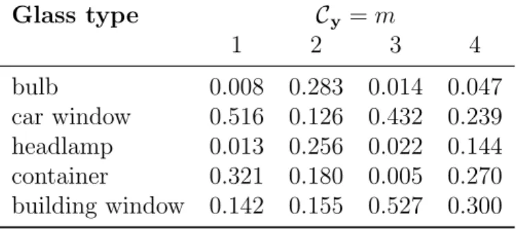
4.1 Use type probabilities. . . 102
4.2 Composite model classification results . . . 106
4.3 Data augmentation classification results. . . 106
4.4 SVM.sub classification results . . . 107
4.5 SVM.full classification results . . . 107
4.6 Composite model expected counts . . . 109
4.7 Data augmentation expected counts . . . 109
4.8 SVM.sub expected counts . . . 110
4.9 SVM.full expected counts . . . 110
4.10 Composite model expected probabilities . . . 112
4.11 Data augmentation expected probabilities . . . 112
4.12 SVM.sub expected probabilities . . . 113
4.13 SVM.full expected probabilities . . . 113
4.14 Classification performance measures . . . 122
5.1 Verbal interpretation ofV . . . 144 xi
5.2 SKL scale for interpretingV . . . 145
5.3 Percentage of FN and FP answers . . . 146
6.1 Example application data file . . . 157
B.1 δtl’s for Metropolis-Hastings moves M-H 2 and M-H 3 . . . 180
C.1 Effective sample size from configuration 1. . . 183
C.2 Standard deviations of covariance matrices from config. 1 . . . 185
C.3 Effective sample size from configuration 3. . . 186
C.4 Standard deviations of covariance matrices from config. 3 . . . 188
C.5 Effective sample size from configuration 4. . . 189
C.6 Standard deviations of covariance matrices from config. 4 . . . 192
D.1 Effective sample size from config. 1 using log-ratios . . . 194
D.2 Log-ratio standard deviations for configuration 1 . . . 197
D.3 Effective sample size from config. 3 using log-ratios . . . 198
D.4 Log-ratio standard deviations for configuration 3 . . . 200
D.5 Effective sample size from config. 4 using log-ratios . . . 201
D.6 Log-ratio standard deviations for configuration 4 . . . 203
E.1 Elemental configurations across use types for simulated data . 205
List of Figures
2.1 Scatterplots of item means for the ratios to oxygen . . . 23
2.2 Standard deviation of each fragment against its mean . . . 24
2.3 Scatterplots of all item means from the database . . . 29
2.4 Scatterplots of the item means with configuration 2 . . . 30
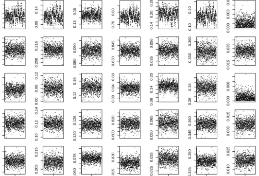
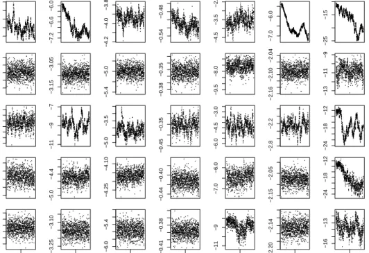
3.1 Trace plots ofθt with the zeros unaltered . . . 46
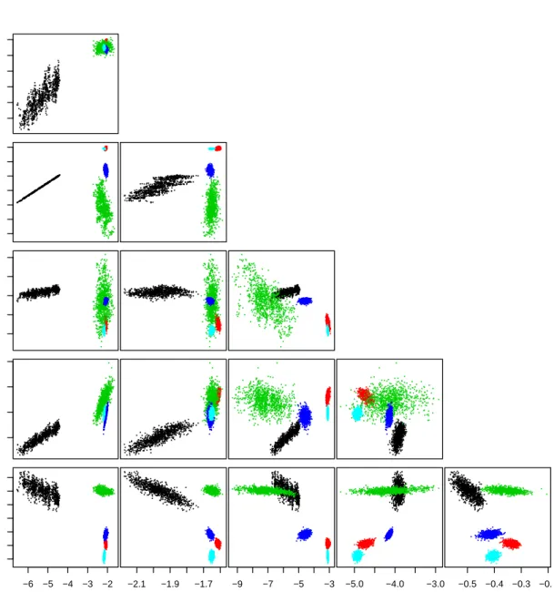
3.2 Scatterplots of θt with the zeros unaltered . . . 47
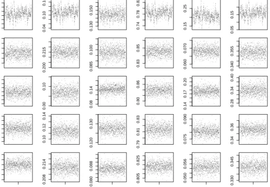
3.3 Trace plots ofθt using data augmentation . . . 53
3.4 Scatterplots of θt for items using data augmentation . . . 54
3.5 Trace plots ofθt for configuration 2 . . . 62
3.6 Scatterplots of θt for items with configuration 2 . . . 63
3.7 Trace plots ofθt using log-ratios . . . 69
3.8 Scatterplots of θt using log-ratios . . . 70
3.9 Log-transformed configuration 2θt trace plots . . . 74
3.10 Log-transformed configuration 2θt scatterplots . . . 75
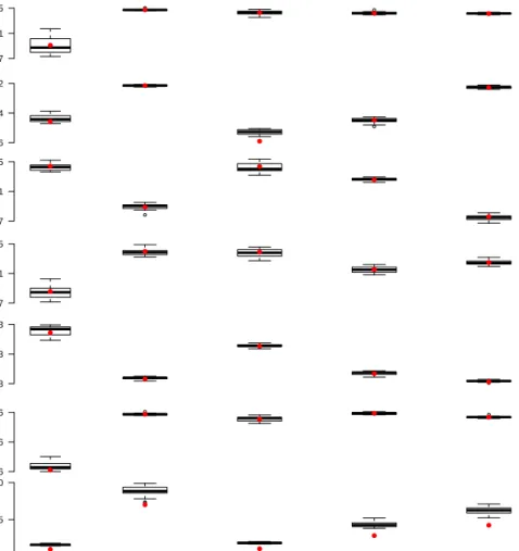
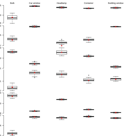
3.11 Boxplots of simulated θt from data augmentation . . . 81
3.12 Boxplots of simulated Ω−1 1 from data augmentation . . . 82
3.13 Boxplots of simulated Ω−21 from data augmentation . . . 83
3.14 Boxplots of simulated Ω−1 3 from data augmentation . . . 84
3.15 Boxplots of simulated Ω−41 from data augmentation . . . 85
3.16 Boxplots of simulated Ω−1 5 from data augmentation . . . 86
3.17 Boxplots of simulated Ψ−1 from data augmentation . . . 87
3.18 Boxplots of simulated Λ−1 from data augmentation . . . 88
3.19 Boxplots of simulated θt for configuration 2 . . . 91
3.20 Boxplots of simulated Ω−1 1 for configuration 2 . . . 92
3.21 Boxplots of simulated Ω−21 for configuration 2 . . . 93
3.22 Boxplots of simulated Ω−1 3 for configuration 2 . . . 94
3.23 Boxplots of simulated Ω−41 for configuration 2 . . . 95
3.24 Boxplots of simulated Ω−1 5 for configuration 2 . . . 96
3.25 Boxplots of simulated Ψ−1 for configuration 2 . . . 97
3.26 Boxplots of simulated Λ−1 for configuration 2 . . . 98
4.1 Composite model posterior probabilities . . . 114
4.2 Data augmentation posterior probabilities . . . 115
4.3 SVM.sub posterior probabilities . . . 116
4.4 SVM.full posterior probabilities . . . 117
5.1 Example histograms of simulatedV values . . . 131
5.2 Example Tippett plots . . . 134
5.3 Example DET curve . . . 135
5.4 Example DET curves and Tippett plots. . . 137
5.5 SPSR plot . . . 139
5.6 ECE example plot . . . 142
5.7 Histogram ofV values from composite model. . . 148
5.8 Histogram ofV values from data augmentation . . . 148
5.9 ROC curve from the composite model . . . 149
5.10 ROC curve from data augmentation . . . 149
5.11 Tippett plots from the composite model . . . 150
5.12 Tippets plots from data augmentation . . . 151 xvi
5.13 DET curves from the composite model . . . 152
5.14 DET curves from data augmentation . . . 152
5.15 ECE plots from the composite model . . . 154
5.16 ECE plots from data augmentation . . . 155
6.1 Snapshot of default application screen. . . 158
6.2 Snapshot of classification application screen . . . 161
6.3 Snapshot of evidence evaluation application screen . . . 164
6.4 Snapshot of evidence evaluation results screen . . . 165
6.5 Application screen for differing configurations . . . 166
A.1 Scatterplots of the item means with configuration 1 . . . 176
A.2 Scatterplots of the item means with configuration 3 . . . 177
A.3 Scatterplots of the item means with configuration 4 . . . 178
C.1 Trace plots ofθt for configuration 1 . . . 183
C.2 Scatterplots of θt for items with configuration 1 . . . 184
C.3 Trace plots ofθt for configuration 3 . . . 186
C.4 Scatterplots of θt for items with configuration 3 . . . 187
C.5 Trace plots ofθt for configuration 4 . . . 190
C.6 Scatterplots of θt for items with configuration 4 . . . 191
D.1 Log-transformed configuration 1θt trace plots . . . 195
D.2 Log-transformed configuration 1θt scatterplots . . . 196
D.3 Log-transformed configuration 3θt trace plots . . . 198
D.4 Log-transformed configuration 3θt scatterplots . . . 199
D.5 Log-transformed configuration 4θt trace plots . . . 201
D.6 Log-transformed configuration 4θt scatterplots . . . 202
E.1 Boxplots of simulated θt for configuration 1 . . . 206
E.2 Boxplots of simulated Ω−1 1 for configuration 1 . . . 207
E.3 Boxplots of simulated Ω−21 for configuration 1 . . . 208
E.4 Boxplots of simulated Ω−1 3 for configuration 1 . . . 209
E.5 Boxplots of simulated Ω−41 for configuration 1 . . . 210
E.6 Boxplots of simulated Ω−1 5 for configuration 1 . . . 211
E.7 Boxplots of simulated Ψ−1 for configuration 1 . . . 212
E.8 Boxplots of simulated Λ−1 for configuration 1 . . . 213
E.9 Boxplots of simulated θt for configuration 3 . . . 214
E.10 Boxplots of simulated Ω−1 1 for configuration 3 . . . 215
E.11 Boxplots of simulated Ω−1
2 for configuration 3 . . . 216
E.12 Boxplots of simulated Ω−31 for configuration 3 . . . 217
E.13 Boxplots of simulated Ω−1 4 for configuration 3 . . . 218
E.14 Boxplots of simulated Ω−1 5 for configuration 3 . . . 219
E.15 Boxplots of simulated Ψ−1 for configuration 3 . . . 220
E.16 Boxplots of simulated Λ−1 for configuration 3 . . . 221
E.17 Boxplots of simulated θt for configuration 4 . . . 222
E.18 Boxplots of simulated Ω−1 1 for configuration 4 . . . 223
E.19 Boxplots of simulated Ω−1 2 for configuration 4 . . . 224
E.20 Boxplots of simulated Ω−31 for configuration 4 . . . 225
E.21 Boxplots of simulated Ω−1 4 for configuration 4 . . . 226
E.22 Boxplots of simulated Ω−1 5 for configuration 4 . . . 227
E.23 Boxplots of simulated Ψ−1 for configuration 4 . . . 228
E.24 Boxplots of simulated Λ−1 for configuration 4 . . . 229
Chapter 1
Introduction
Forensic science is the application of existing sciences to help determine the outcome of an investigation based on the evidence collected. The objective of the forensic scientist, or expert witness, is to quantify the strength of the accumulated evidence found at a crime scene or accident. Most often the evidence gathered in such cases is recovered in the form of traces and is
therefore referred to as trace evidence. All trace evidence collected by the
forensic expert is brought to a forensic laboratory where various measure-ments are recorded for analysis. Common forms of trace evidence found at crime scenes are body fluids and glass fragments. The class of trace evidence
that is of most interest is known as transfer evidence.
Transfer evidence is evidence that has been transferred to or from a crime scene. This can include blood from an assault victim and glass fragments collected from an individual’s clothing, hair or shoes. There are two types of transfer evidence to be considered: that of unknown (questioned) origin and
CHAPTER 1. INTRODUCTION 2
of known origin. For example, glass fragments obtained from a suspect are considered to be of unknown origin as the source of the fragments is
question-able; they are referred to as the recovered sample. Fragments found at the
scene of a crime would usually be of known origin as they are collected from
an on-scene broken source; they are referred to as thecontrol sample (Aitken
and Taroni, 2004). However, control and recovered samples of transfer evi-dence are not always associated with crime scenes and suspects, respectively. For example, a footprint found at a crime scene would be a recovered sample and not a control sample as the footwear that made the print is unknown, and therefore the footprint is of unknown (questioned) origin. The control sample in this case would come from the footwear of a suspect as it would then be of known origin.
A measure of the evidential value or strength of transfer evidence can be com-puted relevant to two complementary propositions: the prosecution propo-sition and the defence propopropo-sition. Three levels of propopropo-sitions comprise a
hierarchy of propositions (Aitken and Taroni, 2004). These are the source
level, activity level and crime level propositions. Source level propositions involve the analysis of control and recovered samples. Here the prosecution proposition would be that the control and recovered samples come from the same source, while the defence proposition would be that the control and recovered samples come from different sources. Activity level propositions include some form of action. For example, the prosecution proposition could be that the suspect assaulted the victim, while the defence proposition would be that the suspect did not assault the victim. Crime level propositions in-volve non-scientific information of interest to the jury, which can include such
CHAPTER 1. INTRODUCTION 3
information as the validity or reliability of eyewitness reports. This thesis will focus on source level propositions involving glass fragments. Chapter
10 of Aitken and Taroni (2004) details how the evidence under evaluation is
computed under these two complementary propostions, with their
terminol-ogy adopted in this thesis. Let E denote the evidence, Hp and Hd denote
the prosecution and defence propositions, and I be additional background
information connected to the case under investigation. The value V of the
evidence forms the likelihood ratio or Bayes factor in favour of the
prosecu-tion proposiprosecu-tion Hp, given the evidence E:
V = Pr(E|Hp, I)
Pr(E|Hd, I)
. (1.1)
The value V in (1.1) can be derived from Bayes’ Theorem which is used to
convert prior beliefs about a proposition, say Hp, to posterior beliefs after
observing some evidence E:
Pr(Hp|E, I) =
Pr(E|Hp, I)×Pr(Hp|I)
Pr(E|I) , (1.2)
where Pr(Hp|E, I) is the posterior probability of Hp given the evidence E,
and Pr(Hp|I) is the prior probability of Hp before observingE. The value of
the evidence V in (1.1) then arises by taking the ratio of (1.2) forHp against
Hd to acquire the posterior odds:
Pr(Hp|E, I) Pr(Hd|E, I) | {z } Posterior odds = Pr(E|Hp, I) Pr(E|Hd, I) | {z } Likelihood ratio (Bayes factor) × Pr(Hp|I) Pr(Hd|I) | {z } Prior odds = V × Pr(Hp|I) Pr(Hd|I) | {z } Prior odds . (1.3)
Prior to receivingE the odds in favour ofHp are given by the prior odds, or
CHAPTER 1. INTRODUCTION 4
beliefs in favour of the prosecution proposition, Hp, into posterior beliefs
in favour of Hp, relative to the defence proposition, Hd, by multiplying the
prior odds by V. Hence, a value of V >1 provides support for Hp, whereas
V <1 provides support for Hd. The way in which V is computed allows for
the evidence to be considered under two complementary propositions, i.e.Hp
andHdare mutually exclusive and exhaustive propositions, while allowing for
other possible factors to be considered during the evaluation of the evidence. The expert witness receives less information about a case than the judge and jury, with their sole purpose to quantify the strength of the evidence, and
so should not be concerned with trying to determine the prior odds (Lucy,
2005). For more information on the evaluation of evidence see Aitken and
Taroni (2004).
The type of forensic evidence that will be analysed within this thesis is on fragments of glass from an experimental database by the Institute of Foren-sic Research, Krakow, which will be referred to as the glass database for the remainder of the thesis. Glass fragments are a common source of trace evi-dence in forensic investigations, with the strength of the evievi-dence evaluated under two complementary propositions as described earlier. Here the pros-ecution proposition would be that the control and recovered samples come from the same glass object, whereas the defence proposition would be that they originated from different glass objects. The main question of interest is then: do the fragments obtained from the suspect come from the glass object found at the crime scene?
As glass fragments collected from a suspect are of unknown origin it would be useful to infer their use type. For example, if a person is involved in an
CHAPTER 1. INTRODUCTION 5
incident such as a car crash or assault where fragments of glass are recov-ered, being able to determine the use type of those fragments could aid a police investigation. Most glass fragments collected for analysis by forensic experts are too small for their use type to be determined by physical
prop-erties such as their thickness or colour (Zadora, 2009), so physico-chemical
measurements, such as the refractive index or elemental composition, are acquired.
Lindley (1977) proposed an approach for continuous measurements in the
form of refractive indices from glass fragments. Here focus is on the el-emental composition of glass. The elel-emental compositions consist of the percentage weights associated with each of the main chemical elements com-prising a glass fragment. As is common with compositional data, many of the recorded weight percentages are zero, indicating those elements’ absence from a fragments composition. Standard statistical procedures developed for analysing compositional data require careful consideration of any zeros present within a composition. The most common approaches to analysing compositional data include transformations involving logarithmic terms, such as the additive log-ratio (alr) and centred log-ratio (clr) transformations of
Aitchison (1986), and the more recently introduced isometric log-ratio (ilr)
transformation of Egozcue et al. (2003). This means that any zeros present
within a composition require special treatment before such transformations can be computed.
This thesis considers two different approaches to handling the compositional zeros. The first method is the most common approach to dealing with zeros as it treats them as rounded zeros. Rounded zeros indicate that an element
CHAPTER 1. INTRODUCTION 6
is present within a fragment but that traces of that element are below the detection limit of the measuring equipment. This method essentially updates any zeros with non-zero values that are below limits of detection. The second method treats the zeros as essential zeros, indicating the absolute absence of
that element from a fragment’s composition (Mart´ın-Fern´andezet al.,2003).
This method is similar to that of Stewart and Field (2011) in that the glass
data is partitioned depending on whether elements are present or absent from each glass composition. This can lead to a reduction in the dimension of the data, and to the modelling of subcompositions.
The methods of dealing with zeros mentioned above will be incorporated into a Bayesian hierarchical model. The model takes into consideration the glass use type and the hierarchical structure of the glass data by including three levels of variability. The model is then used to classify glass items into one of five use type categories and for computing the evidential value of glass fragments relating to two competing propositions.
1.1
Overview of thesis
Chapter 2provides a review of current methods used in the analysis of
com-positional data, as well as a detailed description and exploratory analysis of
the glass database. Chapter 3 details the Bayesian hierarchical model and
the Markov Chain Monte Carlo (MCMC) implementation, and also describes the two different approaches taken to handling the many compositional zeros
present in the glass database. Chapter 3 also presents the posterior draws
clas-CHAPTER 1. INTRODUCTION 7
sification procedure and results of classifying all glass items in the database
are detailed in Chapter4, while the evaluation of glass fragments as evidence
is described, including the results, in Chapter 5. Chapter 6describes a web
application of the classification and evidence evaluation approaches along with instructions on how to load the data into the application. Discussion
Chapter 2
Compositional data
As already mentioned in the introduction, the glass database contains mea-surements on percentage weights and so is compositional in nature. This chapter will begin with an overview of statistical methods for compositional data and the techniques used to analyse it before going on to later detail the glass database itself.
Compositional data commonly occurs in scientific disciplines such as chem-istry, geology, economics, and many others. Compositional data are vectors comprised of non-negative parts of some whole. The sample space or simplex
as defined by Aitchison (1986) is SD−1 = ( w= (w1, . . . , wD) :wd≥0; D X d=1 wd=c ) , (2.1)
wherecis the constant sum constraint and value of the full composition, i.e.
c = 1,100, . . . for proportions, percentages etc. The simplex has the vector operations of perturbation and power transformation which are analagous to
CHAPTER 2. COMPOSITIONAL DATA 9
translation and scalar multiplication in RD.
The perturbation operation can be used to record changes in a composition.
If x is a D-part composition consisting of decaying components and u is
a D-part vector containing the decay rates of x, then the newly perturbed
composition y can be written as
y=x⊕u=C(x1u1, . . . , xDuD). (2.2)
The closure operator C used in (2.2) is defined as
C(x) = PDc
d=1xd
x, (2.3)
and is used to convert raw composition measurements into proportions,
per-centages etc. depending on the choice of c. The vector u containing any
change or perturbation in a composition can be found from the inverse op-eration:
u=yªx=C(y1/x1, . . . , yD/xD), (2.4)
with u = 1D the neutral element corresponding to no change from x to y.
The perturbation operation allows for compositional measurements collected from a source, that may be represented in different units, to produce the same qualitative results under statistical analyses if there exists a perturbing
vector u that allows for easy transformations between units. The power
transformation can also be used to rescale a composition given some constant
a:
y=a⊗x=C(xa
CHAPTER 2. COMPOSITIONAL DATA 10
An analogue to the Euclidean distance in the simplex, known as Aitchison
distance (Aitchison,1986), is defined by
da(x,y) = " 1 D X i<j µ lnxi xj −lnyi yj ¶2#1/2 = " D X i=1 µ ln xi g(x)−ln yi g(y) ¶2#1/2 , (2.6)
where g(x) = (x1· · ·xD)1/D is the geometric mean of x. The Aitchison
dis-tance satisfies the property of subcompositional dominance (Aitchison,1992).
Subcompositional dominance is the property whereby the distance between
two full compositions x and y is at least as large as the distance between
any two subcompositionsx∗ andy∗, i.e.d
a(x,y)≥da(x∗,y∗). There are two
principles of compositional data to consider before carrying out any analysis.
These are scale invariance and subcompositional coherence (Aitchison and
Egozcue, 2005).
Compositional vectors w1 and w2 are considered compositionally equivalent
if C(w1) = C(w2), which implies the existance of a proportionality constant,
λ, such that w1 =λ·w2. A functionf is said to be scale invariant if
f(w1) =f(λ·w1). (2.7)
Since scale invariance is satisfied by taking the ratio of D−1 components
to the Dth component of a composition, and as compositions carry relative
information, compositional data are most often expressed in terms of ratios of the component parts. A function is also said to be permutation invariant if it is unaffected by changes to the ordering of the component parts.
For any subset S of the indices (1, . . . , D) of a D-part composition such that
CHAPTER 2. COMPOSITIONAL DATA 11
should be equal to the corresponding ratio in the full composition w:
si
sj
= wi
wj
∀ (i, j ∈S). (2.8)
This is referred to as subcompositional coherence, and along with scale in-variance, is the reason why analyses of compositional data regularly involve the use of component ratios. The use of ratios also removes the constant sum constraint of the simplex allowing for the use of standard multivariate techniques, and for the dimension of the data to be reduced by one. Typi-cally data transformations are then applied to the ratios to improve variance stability and normality.
2.1
Transformations
2.1.1
Additive log-ratio
The most common transformation applied to compositional data was
intro-duced by Aitchison (1982) and involves taking the logarithm of D−1
com-ponents to the remaining one. This is referred to as the additive log-ratio (alr) transformation: alr(w) = µ ln µ w1 wD ¶ , . . . ,ln µ wD−1 wD ¶¶ . (2.9)
The alr transformation removes the sum constraint allowing for the appli-cation of standard multivariate techniques, such as assuming the data to be multivariate normally distributed, where the variance-covariance matrix, Σ,
CHAPTER 2. COMPOSITIONAL DATA 12
would be of dimension (D−1)×(D−1) and given as
Σ = · cov ½ ln µ wi wD ¶ ,ln µ wj wD ¶¾ : i, j = 1, . . . , D−1 ¸ . (2.10)
The alr transformation satisfies the principles of compositional data described earlier, but it is not without its issues. One potential issue is that it does
not treat the parts of w symmetrically with wD taking on the role of the
common divisor in the log-ratios. Also, despite the invariant property, the
choice of the common divisor wD in the ratio still has an important role
to play in terms of the goodness of fit to normality of the log-transformed
data (Rayens and Srinivasan, 1991a). The component chosen as the divisor
needs to be greater than zero within a composition in order to avoid further complications involving compositional zeros.
Baxteret al.(2005) point out that performing a principal component analysis (PCA) on the standardised ratios recovers the structure of the data much better than using the alr transformed data. This is due to component parts with very low absolute values and high variability strongly influencing the
structure of the log-transformed data; see also Wang et al. (2008). The alr
transformation also requires that all component parts be strictly positive, but zero measurements occur frequently in compositional data, leading to the development of strategies to deal with the presence of such values. These
strategies are detailed in Section 2.2.
2.1.2
Centred log-ratio
Another transformation proposed byAitchison (1986) that satisfies the
CHAPTER 2. COMPOSITIONAL DATA 13
clr transformation is the logarithm of the ratio of all D-parts to their
geo-metric mean: clr(w) = µ ln µ w1 g(w) ¶ , . . . ,ln µ wD g(w) ¶¶ , (2.11)
whereg(w) is the geometric mean. Unlike the alr, the clr treats compositions
symmetrically by not having a component singled out as the common divisor.
For the clr, theD×Dvariance-covariance matrix, Γ, of aD-part composition
w is given as Γ = · cov ½ ln µ wi g(w) ¶ ,ln µ wj g(w) ¶¾ : i, j = 1, . . . , D ¸ . (2.12)
An advantage the clr has over the alr is being able to visualise allD-parts of a
composition when performing an exploratory analysis of the data (Campbell
et al.,2009). However, as (2.12) is singular, it is simpler to revert back to the alr transformation when using standard methods requiring the inverse of the
variance-covariance matrix, similarly to howCampbellet al.(2009) analysed
data on New Zealand nephrite.
2.1.3
Isometric log-ratio
Egozcue et al. (2003) introduced the isometric log-ratio (ilr) transformation for compositional data which allows for angles and distances in the simplex to be associated with angles and distances in real space. The ilr transformation
is given as ilr(w) =x= (x1, . . . , xD−1)∈RD−1 where
xi = 1 p i(i+ 1)ln ÃQi j=1wj (wi+1)i ! . (2.13)
The relationships between the ilr and the alr and clr transformations are
CHAPTER 2. COMPOSITIONAL DATA 14
Other logarithmic transformations that have been applied to compositional
data include the complementary log-log transformation (Neocleous et al.,
2011) and the multiplicative log-ratio (mlr) transformation (Stewart and
Field,2011). However, as previously stated, in order to compute logarithmic transformations all component parts must be strictly positive. This has led to the proposal of non-logarithmic transformations for compositional data.
2.1.4
Box-Cox family
Rayens and Srinivasan (1991a) propose using the family of transformations
considered by Box and Cox (1964) to improve the fit to normality of
com-positional data. Rayens and Srinivasan believe that the ratio transformation alone alleviates most of the issues concerning the statistical analysis of com-positional data, with the additional logarithmic transformation used mainly to improve normality. As the log transformation is part of the Box-Cox fam-ily of transformations, a better fit to normality, and thus a better use of normal based multivariate techniques, should be achievable by considering the whole family of transformations.
Letxbe the ratios ofD−1 components to the remaining one. The Box-Cox
transformation is then applied to each component of xas follows
yi = xλii −1 λi , if λi 6= 0, ln(xi), if λi = 0, (2.14)
where λ= (λ1, . . . , λD−1) are the power parameters of the transformation.
CHAPTER 2. COMPOSITIONAL DATA 15
subcompositional analysis with the use of non-logarithmic transformations. However, they believe this concern can be resolved in practice if an ever present component is commonly accepted by practitioners to be the common divisor.
Application of the Box-Cox and alr transformations to real data in Rayens
and Srinivasan (1991a) show improvements in goodness of fit to
normal-ity in favour of the Box-Cox transformation. Rayens and Srinivasan ex-tend their application of the Box-Cox transformation in parametric and
non-parametric approaches to modelling compositional data inRayens and
Srini-vasan (1991b).
2.1.5
Hypersphere
Wanget al.(2007) andNeocleouset al.(2011) avoid the complication of zero components by applying a hyperspherical transformation to compositional
data. First the square root is applied to all D-parts of a compositionw:
sqrt(w) = (√w1, . . . ,
√
wD), (2.15)
transforming it onto the surface of the (D−1)-dimensional hypersphere. The
Cartesian coordinates of (2.15) are then mapped to polar coordinates using
a recursive relationship. Scealy and Welsh (2011) used (2.15) to allow for
directional data distributions - such as the Kent distribution - to be used
when modelling compositional data; see also Scealy and Welsh (2014).
Regardless of which transformation is applied to compositional data, there still lies the problem pertaining to zeros, especially in datasets where they
CHAPTER 2. COMPOSITIONAL DATA 16
are abundant. However, zeros are still notably more problematic for any of the logarithmic transformations, with even a small number of zeros caus-ing computational issues; they also have a stronger influence on the data
distribution, as will be demonstrated in Section 2.3.
2.2
Compositional zeros
Zero measurements occur frequently in compositional data causing problems with the application of any of the logarithmic transformations mentioned in
Section 2.1. There are two types of compositional zeros: rounded zeros,
in-dicating the presence of a component but below some detection limit; and essential zeros, denoting the absolute absence of a component from an
ob-servation (Mart´ın-Fern´andez et al., 2003). Different approaches have been
adopted for both types of zeros.
2.2.1
Rounded zeros
Non-zero traces of components that are below limits of detection for some measuring equipment are reported as zero concentrations and referred to as rounded zeros. The simplest strategy then is to replace rounded zeros by
some small constant equal to or below the detection limit (Neocleous et al.,
2011). To satisfy the constant sum constraint the non-zero components would
then have to be adjusted accordingly, which can be done using one of several techniques.
CHAPTER 2. COMPOSITIONAL DATA 17
Simple replacement strategy
The easiest of such zero replacement techniques is known as the simple
re-placement strategy (Mart´ın-Fern´andez and Thi´o-Henestrosa, 2006). A D
-part composition wcontaining rounded zeros is replaced by an updated
non-zero composition u: ud= c c+P{k:wk=0}δkδd, if wd = 0, c c+P{k:wk=0}δkwd, if wd >0, (2.16)
wherec=Pwdis the constant sum constraint, and δis a value below limits
of detection.
Additive replacement strategy
Aitchison (1986) proposed an additive replacement strategy where any D
-part composition w, containingZ zeros is replaced by an updated non-zero
composition u: ud = δ(Z+1)(D−Z) D2 , if wd= 0, wd− δ(ZD+1)2 Z, if wd>0, (2.17)
where δ is a value smaller than the given threshold of the measuring
equip-ment. A problem with this strategy is that it fails to preserve the ratios
between components of the original composition w and the updated
non-zero composition u, leading to subcompositional incoherence. This led to
other replacement strategies being proposed with Fry et al. (2000) adopting
CHAPTER 2. COMPOSITIONAL DATA 18
dealing with share ratios in economic data, and to the introduction of the
multiplicative replacement strategy of Mart´ın-Fern´andez et al. (2000).
Multiplicative replacement strategy
The zero replacement technique of Mart´ın-Fern´andez et al. (2000) does not
rely on the number of components D, or the number of zerosZ, but only on
the given threshold value δ:
ud = δd, if wd= 0, wd−wcd P {d:wd=0}δd, if wd>0, (2.18)
where c=Pwd is the constant sum constraint. This proposed replacement
strategy preserves the ratios between the old observations w, and the newly
adjusted observations u. Sanford et al. (1993) suggest values equal to 0.55
times the threshold δ be used when imputing values below limits of
detec-tion. A comparison of the performance of the additive and multiplicative
replacement strategies can be found in Mart´ın-Fern´andez et al. (2003).
Although the multiplicative replacement strategy preserves ratios it can run into problems with compositional datasets containing a large number of zeros
(more than 10% (Sanford et al., 1993)). The issue of artificial correlation
induced by the strategy for datasets containing a large proportion of zeros is
raised in Palarea-Albaladejoet al. (2007).
Palarea-Albaladejo et al. (2007) propose a parametric approach to replac-ing components below the limits of detection in the presence of many zero
algo-CHAPTER 2. COMPOSITIONAL DATA 19
rithm that takes into account that rounded zeros are seen as missing values (Mart´ın-Fern´andez and Thi´o-Henestrosa,2006), however they are not consid-ered missing at random (MAR), but below limits of detection, so are therefore treated as not missing at random (NMAR). Their method also takes into ac-count the covariance structure of the data ensuring imputed values for zeros of the same component differ from one another, thus reducing the artificial correlation induced by the multiplicative replacement strategy.
2.2.2
Essential zeros
Essential zeros are different to rounded zeros in that they are not zero due to limits of detection, but considered to be actual zeros. Essential zeros appear in compositions in disciplines such as economics. Most often zeros in compositional data are treated as rounded zeros and so fewer advancements
have been made for zeros considered to be essential. Aitchison and Kay
(2003) believe that such zero problems may not exist once the precise aims of
a study of compositional data containing essential zeros have been obtained.
Zadora et al. (2010) modelled non-zero subcompositions using a two stage model approach, with the presence of zeros treated using an independent
bi-nary model as suggested by Aitchison and Kay (2003). Bacon-Shone (2003)
explores the problem of essential zeros arising in household expenditure data, i.e. households who spend money on alcohol versus those that do not. Bacon-Shone suggests the use of multivariate logistic or probit models for modelling
the essential zero structure within the data. Butler and Glasbey (2008) and
CHAPTER 2. COMPOSITIONAL DATA 20
Gaussian random variable in their models, that has the effect of creating
a point mass at zero. Stewart and Field (2011) developed mixture models
for compositional data containing zeros when examining the diets of preda-tors. Stewart and Field partitioned their data depending on whether different species were present or absent from a predator’s diet, thus only modelling
the non-zero components. Stewart(2013) adapted the model using the
zero-inflated beta distribution, simplifying the previous approach by not having to apply the multiplicative log-ratio transformation to the same data set.
Daunis-i-Estadellaet al.(2008) introduce the idea of a different type of com-positional zeros that occur in count data sets. Referring to them as count
zeros, Daunis-i-Estadella et al.propose the use of the multiplicative
replace-ment strategy in order to preserve ratios between prior and posterior counts when the Dirichlet distribution is used as the conjugate prior of the multi-nomial distribution within a Bayesian framework, thus allowing for the ap-plication of the alr transformation. The glass database will now be detailed, where its unique aspects are highlighted during an exploratory analysis that is informative about the approaches used in its analysis.
2.3
Glass database
The glass database being analysed consists of measurements obtained from an experimental setting, and was provided by Prof. G. Zadora of the Institute of Forensic Research, Krakow. The database is comprised of four fragments -each having three replicate measurements – from 320 glass items to give a to-tal of 3840 measurements. The 320 glass items are split across five use types:
CHAPTER 2. COMPOSITIONAL DATA 21
26 bulbs, 94 car windows, 16 headlamps, 79 containers and 105 building win-dows. The elemental content of each fragment was obtained from a scanning electron microscope with an energy dispersive X-ray (SEM-EDX) spectrom-eter. The fragments chosen for analysis were obtained from an experimental setting by breaking a glass item of a specified use type into smaller fragments. The fragments with the smoothest and flattest surfaces with linear
dimen-sion less than 0.5 mm were then selected for analysis (Zadora, 2009). The
measurements produced by SEM-EDX are on the percentage weights (wt%) – to two decimal places – of the main elements comprising each fragment’s composition. These main chemical elements are: oxygen (O), sodium (Na), magnesium (Mg), aluminium (Al), silicon (Si), potassium (K), calcium (Ca) and iron (Fe). Other methods of elemental analysis of glass fragments in-clude non-destructive energy dispersive X-ray microflourescence (microXRF) (Hickset al.,2003) and laser ablation inductively coupled plasma mass
spec-trometry (LA-ICP-MS) (Trejos and Almirall,2005).
The percentage weights of each fragment are compositional and therefore are non-negative and sum to 100%. Let the number of elements in a fragment’s
composition be D. The percentage weights are then denoted by the D
di-mensional vector w = (w1, . . . , wD), with wd ≥ 0 and
PD
d=1wd = 100. To
remove the sum constraint the elements can be transformed into a (D−1)
dimensional vector of ratios by taking the ratio of (D−1) elements to the
Dth element. The transformed vector is
w∗ = µ w1 wD , . . . ,wD−1 wD ¶ , (2.19)
where oxygen was chosen as the common divisor, wD, due to having the
CHAPTER 2. COMPOSITIONAL DATA 22
A number of the percentage weights are zero with their prevalence
differ-ing across elements, as shown in Table 2.1. Figure 2.1, containing plots of
the item means for the ratios to oxygen, illustrates how a large number of compositional zeros can influence the distribution of the data.
Table 2.1: Frequency of zero measurements by chemical element.
Element O Si Na Ca Al Mg K Fe
Frequency 0 0 0 108 205 265 1168 3036
Percentage 0.0 0.0 0.0 2.8 5.3 6.9 30.4 79.1
In order to improve variance stability and normality, a transformation was
then applied to the ratios in (2.19). In addition to the additive log-ratio
transformation, members from the family of transformations ofBox and Cox
(1964) were examined, with improvements in variance stability and
normal-ity of the data obtained by applying the square root to (2.19). Figure 2.2
contrasts the alr and square root transformations, and shows that the square root transformation improves variance stability in the data more so than the alr transformation. This is due to the chemical elements with many zeros and very low weight percentages having a much stronger influence over the log-transformed ratios than those of the square root. Not only is the square root transformation more effective at stabilising the variability in the data, it also does not require any zeros be altered in order to be computed. Due to these reasons the square root transformation has been chosen as the appropriate transformation for the analysis of the glass database.
CHAPTER 2. COMPOSITIONAL DATA 23 0.10 0.20 Na 0.00 0.03 0.06 Mg 0.00 0.02 0.04 Al 0.4 0.6 0.8 Si 0.00 0.06 0.12 K 0.000 0.006 0.012 0.00 0.10 0.20 Fe Ca 0.10 0.20 Na 0.00 0.03 0.06 Mg 0.00 0.02 0.04 Al 0.4 0.6 0.8 Si 0.00 0.04 0.08 0.12 K Figure 2.1: Scatterplots of the ratios to oxygen for all item means from the
database. The different coloured points correspond to the five use type categories: bulb,car window,headlamp,containerandbuilding
CHAPTER 2. COMPOSITIONAL DATA 24 −8 −6 −4 −2 0 0.0 0.5 1.0 1.5 2.0 2.5 3.0
Mean of each fragment
sd of each fr agment Na Mg Al Si K Ca Fe 0.0 0.2 0.4 0.6 0.8 1.0 0.00 0.02 0.04 0.06 0.08 0.10
Mean of each fragment
sd of each fr agment Na Mg Al Si K Ca Fe
Figure 2.2: Plots of fragments’ standard deviations against corresponding means, using the alr (left panel) and the square root (right panel) transformations. For the alr, 0.005 was added to all compositional zeros. Seven elemental pairs (mean, sd) are plotted for each frag-ment, computed using the fragment’s three repeated measurements. While the variability is roughly the same across the range of mean levels for the square root transformed data, the range of sd’s changes considerably across mean levels for the alr transformed data.
Despite the square root transformation improving normality and stabilising the variability in the data, the presence of many zeros still has a bearing on the distribution of the data. One way to reduce the influence of the zeros is to partition the glass data depending on whether an element is present or
absent from a glass item’s composition. This reduces (2.19) from a (D−1)
dimensional composition to a (D−Z −1) dimensional subcomposition by
eliminating the Z zero elements.
CHAPTER 2. COMPOSITIONAL DATA 25
an item’s composition is when it comes to determining that item’s use type. For example, the database has no bulbs or headlamps containing iron, and so if a composition containing iron is observed then it is unlikely that it is either of these two use types. Three elements are always present in glass: oxygen, silicon and sodium. The remaining five can be present or absent from the
composition of a glass item, which gives 25 = 32 possible configurations of
the elements according to their presence or absence. Ten of the possible 32
configurations were observed in the glass database, as shown in Table2.2. As
can be seen from Table2.2, most of the configurations account for very few of
the items in the database. The elements iron and potassium are accountable
for 87.9% of the zero measurements in the database, as seen in Table 2.1,
therefore most of the zeros present in the database can be removed by only focusing on the presence or absence of these two elements. Therefore only
four configurations are later considered as shown in Table 2.3, where some
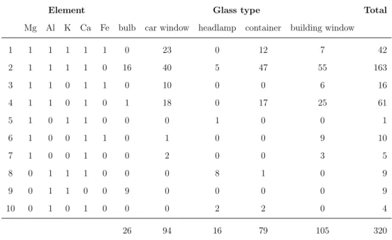
CHAPTER 2. COMPOSITIONAL DATA 26
Table 2.2: Presence (1) and absence (0) of elements at item level by use type.
Element Glass type Total
Mg Al K Ca Fe bulb car window headlamp container building window
1 1 1 1 1 1 0 23 0 12 7 42 2 1 1 1 1 0 16 40 5 47 55 163 3 1 1 0 1 1 0 10 0 0 6 16 4 1 1 0 1 0 1 18 0 17 25 61 5 1 0 1 1 0 0 0 1 0 0 1 6 1 0 0 1 1 0 1 0 0 9 10 7 1 0 0 1 0 0 2 0 0 3 5 8 0 1 1 1 0 0 0 8 1 0 9 9 0 1 1 0 0 9 0 0 0 0 9 10 0 1 0 1 0 0 0 2 2 0 4 26 94 16 79 105 320
Table 2.3: Presence (Fe, K) and absence (Fe,K) at item level by use type.
Glass type Configuration m Total
1: Fe, K 2: Fe, K 3: Fe, K 4: Fe, K
bulb 0 25 0 1 26 car window 23 40 11 20 94 headlamp 0 14 0 2 16 container 12 48 0 19 79 building window 7 55 15 28 105 42 182 26 70 320
Just from observing an item’s composition it is obvious which elements are present and which are absent: only eight of the 320 items have an element where all 12 measurements are neither all positive nor zero, as shown in
Ta-CHAPTER 2. COMPOSITIONAL DATA 27
ble 2.4. Here an element is assumed to be present in an item’s composition
if at least one of its 12 measurements is positive. Of the eight items in Table
2.4 five of them contain measurements on iron or potassium that are neither
all positive nor zero. For those five items 28/120 of the total measurements
associated with the elements iron and potassium are zero. Under the as-sumption that an element is present if at least one of its measurements is
positive this means that 28/4204 = 0.7% of zero measurements would ‘slip
by’ when observing the presence or absence of these two elements. Also,
across all eight of the items in Table 2.4 containing an element with its 12
measurements not all positive or all zero, these zeros account for only 0.9% of zeros in the entire glass database, and so the assumption that an element is present if at least one measurement is positive seems reasonable.
Table 2.4: Frequency of items containing chemical elements where all 12 mea-surements are neither all positive nor zero.
Glass type Element Total
Mg Al K Ca Fe
car window 0 1 0 0 2 3
building window 1 1 3 0 0 5
Total 1 2 3 0 2 8
Taking into account the presence or absence of elements should improve normality assumptions when it comes to modelling the data by decreasing the influence of the zeros on the distribution of the data. This can be seen
by comparing Figure 2.3, containing plots of the means at item level for all
items in the database, with Figure 2.4, containing plots of the item means
CHAPTER 2. COMPOSITIONAL DATA 28
The next chapter discusses a Bayesian hierarchical model for the glass data. It also details the two different approaches taken to dealing with the many compositional zeros. The first approach assumes all of the compositional ze-ros are due to the concentrations of those elements being below the limits of the detection equipment, and updates the zeros during the modelling proce-dure with values below this detection limit. The second approach focuses on using the four configurations mentioned above by separating the data into four distinct subsets according to the presence or absence of the elements iron and potassium. This gives four separate models for this approach that are then brought together to form a single model.
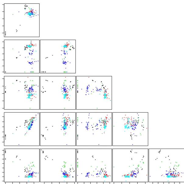
CHAPTER 2. COMPOSITIONAL DATA 29 0.30 0.40 0.50 Na 0.00 0.10 0.20 Mg 0.00 0.10 0.20 Al 0.65 0.80 Si 0.00 0.15 0.30 K 0.00 0.04 0.08 0.12 0.0 0.2 0.4 Fe Ca 0.30 0.40 0.50 Na 0.00 0.10 0.20 Mg 0.00 0.10 0.20 Al 0.65 0.75 0.85 Si 0.00 0.15 0.30 K Figure 2.3: Scatterplots of the square root transformed ratios of all item means
from the database. The different coloured points correspond to the five use type categories: bulb,car window,headlamp,container and
CHAPTER 2. COMPOSITIONAL DATA 30 0.30 0.40 0.50 Na 0.00 0.10 0.20 Mg 0.00 0.10 0.20 Al 0.65 0.75 0.85 Si 0.0 0.1 0.2 0.3 0.4 0.00 0.10 0.20 0.30 Ca K 0.30 0.40 0.50 Na 0.00 0.10 0.20 Mg 0.00 0.10 0.20 Al 0.65 0.75 0.85 Si Figure 2.4: Scatterplots of the square root transformed ratios of the item means
for items with configuration 2 from Table2.3. The different coloured points correspond to the five use type categories: bulb, car window, headlamp,containerand building window.
Chapter 3
Models
The elemental content of glass fragments has been previously modelled by
Aitken and Lucy (2004) and Neocleous et al. (2011) from a frequentist per-spective. The models proposed were random effects models incorporating two levels of variation: between-item and within-item. The between-item level variability is captured by a random effect associated with individual glass items, and the within-item variability by a random effect associated
with individual fragments from the same glass item. Aitken and Lucy(2004)
performed their analysis on building windows using the logarithm of three
different ratios believed to be the most discriminatory for such data.
Neo-cleous et al. (2011) used log-ratios for the entire elemental composition of glass, with oxygen chosen as the common divisor. Along with the log-ratio
transformation, Neocleous et al. (2011) also used a complementary log-log
transformation – logarithm of the negative log-ratio transformation – and a spherical transformation mapping the elemental composition onto the unit
CHAPTER 3. MODELS 32
hypersphere. In terms of results, there was no single transformation
outper-forming the others. For instance under the normal model used by Neocleous
et al. (2011), the spherical transformation yielded the lowest false positive rate, while the log-ratio transformation yielded the lowest false negative rate. Here a Bayesian approach is used to model the hierarchical structure of the data using a mixed effects model. As the hierarchical structure of the data contains an additional layer relating to the repeated measurements on each fragment, an additional random effect is placed at this measurement error level on top of the two levels of variability already mentioned. The model is a mixed effects model and not a random effects model as it also includes a fixed effect term for the overall mean for each glass type. For a detailed
introduction to mixed effects models see Pinheiro and Bates(2000). See also
Gelman et al.(2004) for details on hierarchical models in a Bayesian
frame-work. As was seen from the exploratory analysis in Chapter 2 the square
roots of the compositional ratios improved normality and stability in the data variability more so than the log-ratios. Therefore the primary transfor-mation used when analysing the glass database will be the square roots of the compositional ratios, with oxygen chosen as the common divisor. Also, unlike the log-ratio transformation, the square root transformation does not require any zeros present in the data to be altered. Results from the model using the log-ratio transformation will also be produced for comparison’s sake, and to demonstrate why it does not perform as well as the square root transformation.
CHAPTER 3. MODELS 33
3.1
Bayesian hierarchical model
Denote the square root ratios for each glass measurement by ztijk, where
ztijk is the k-th replicate measurement from the j-th fragment of the i-th
glass item of use type t. The dimension p of ztijk at item level may differ
across the elemental configurations detailed in Section2.3when the approach
to modelling the presence or absence of the elements iron and potassium is
taken; see Section 3.2.3. It is then assumed that
ztijk =θt+bti+ctij +²tijk,
bti iid∼Np(0,Ωt−1), ctij iid∼Np(0,Ψ−1), ²tijk ∼iidNp(0,Λ−1).
(3.1)
The fixed effect term for the mean of use typet is denoted by the parameter
θt; the item-level random effect by bti; the fragment within-item random
effect byctij; and the error at measurement level by²tijk. Each of the random
effects are assumed to have multivariate normal distributions, with unknown
precision matrices Ωt, Ψ and Λ. The separate covariance matrices, Ω−t1, were
introduced at item level for each use type after observing dissimilar levels of random variability between items of differing use types, which will be seen from the model results. The assumption of normality is questionable and may
not hold after looking at scatterplots of the data in Chapter2, even when the
zero concentrations are removed. However, the validity of this assumption did not have any substantial affect on the conclusions drawn from the models used, as seen from the results of classification and evidence evaluation in
chapters4and5. Misspecifying random effects distributions does not greatly
affect estimations of the random effects variances (McCulloch and Neuhaus,
CHAPTER 3. MODELS 34
θ = {θt}Tt=1; b = {bti}Ii=1t Tt=1; c = {ctij}Jj=1 Ii=1t Tt=1 and Ω = {Ωt}Tt=1. Here
T = 5 denotes the number of use types in the database; It denotes the
number of glass items of each use type t (I1 = 26, I2 = 94, I3 = 16, I4 = 79,
I5 = 105);J = 4 denotes the total number of fragments associated with each
item; andK = 3 is the number of replicate measurements on each fragment.
For a glass item z of use type Tz = t with JK measurements, model (3.1)
implies - without conditioning on the random effects - that the distribution
of item z is
z|Tz =t, ξ ∼NJKp(1JK⊗θt, Σt), (3.2)
where ξ = {θ,Ω,Ψ,Λ} collectively denotes the model parameters. When
modelling the presence and absence of iron and potassium the model
param-eters for the subset of items with configurationmin Table2.3will be denoted
by ξm. The covariance matrix Σt is given by
Σt = (1JK10JK)⊗Ω−t1+ [IJ ⊗(1K10K)] ⊗Ψ−1 +IJK⊗Λ−1, (3.3)
where1ddenotes a column vector ofd1’s, andIdis thed×didentity matrix.
The prior distributions placed on the fixed effects θt are also assumed
inde-pendent multivariate normals, but they are restricted to the positive orthant, in order to ensure that the square root transformed means are non-negative:
θtiid∼Np(0,Φ−1), θt >0, t= 1, . . . , T. (3.4)
The covariance matrix, Φ−1, of the fixed effects is fixed and set equal to
s · Ip, where s is a relatively large constant. All subsequent results used
the value s = 1000. This gives a priori independent components of θt with
CHAPTER 3. MODELS 35
corresponding sample means. The precision matrices for the random effects have conjugate Wishart hyperpriors placed on each of them:
Ωt∼Wp(d1t, At), Ψ∼Wp(d2, B), Λ∼Wp(d3, C), (3.5)
where d1t, d2 and d3 denote the degrees of freedom; and At, B and C are
precision matrices. The degrees of freedom of the Wishart distribution need
to be greater than the data dimension minus one, e.g.d2 > p−1, so
noninfor-mative prior values for the degrees of freedom are set equal top; seeDeGroot
(1970) for details on the Wishart distribution. The precision matrices At,
B and C are all set equal to (1/1000)·Ip so that, as mentioned for the θt’s
above, posterior inferences would be largely driven by the data.
3.1.1
Markov Chain Monte Carlo implementation
In Bayesian inference Markov Chain Monte Carlo (MCMC) methods are used to simulate and draw samples from distributions of interest. Monte Carlo methods are used to approximate integrals and closed-form expressions that are otherwise extremely difficult or impossible to evaluate. This is done by creating a Markov chain which, after reaching a state of equilibrium, is effectively sampling from the desired target distribution. This is an iterative algorithm procedure that after a period of time will have produced a chain consisting of samples drawn from the target distribution.
The two most frequently used MCMC algorithms are the Gibbs sampler and the Metropolis-Hastings algorithm. Depending on the model, only one of the sampling techniques may be required, but it is also possible to have a hybrid
CHAPTER 3. MODELS 36
sampling technique that uses both methods. As the core of the sampler used here is Gibbs sampling, the Gibbs sampler will be described first, before then going on to look at the Metropolis-Hastings algorithm and the corresponding moves incorporated into the sampler.
Gibbs sampling
Since the full conditional distributions of the random effects {b,c} and the
parameters of ξ = {θ,Ω,Ψ,Λ} - minus θ with its applied restriction - are
known standard distributions, Gibbs sampling moves can be used to update these parameters. Gibbs sampling moves work by generating values from the full conditional distribution of a variable, i.e. the conditional distribution of a variable given all other variables. For example, let the vector containing all
parameters of interest be ζ = (ζ1, . . . , ζn)0, then the Gibbs sampler operates
as follows:
1. First set initial values for the parametersζ0 = (ζ0
1, . . . , ζn0)0
2. Iteratively generate values for ζ where the first iterate is generated as
follows: ζ11 ∼p(ζ11 |ζ20, . . . , ζn0) ζ21 ∼p(ζ21 |ζ11, ζ30, . . . , ζn0) ζ1 3 ∼p(ζ31 |ζ11, ζ21, ζ40, . . . , ζn0) ... ζ1 n∼p(ζn1 |ζ11, . . . , ζn1−1)