Original Citation:
Matching under Preferences
Cambridge University Press Publisher:
Published version: DOI:
Terms of use: Open Access
(Article begins on next page)
This article is made available under terms and conditions applicable to Open Access Guidelines, as described at http://www.unipd.it/download/file/fid/55401 (Italian only)
Availability:
This version is available at: 11577/3281635 since: 2018-10-21T22:41:32Z
Matching under Preferences
Bettina Klausa, David F. Manloveb and Francesca Rossic14.1 Introduction and discussion of applications
Matching theory studies how agents and/or objects from different sets can be matched with each other while taking agents’ preferences into account. The theory originated in 1962 with a celebrated paper by David Gale and Lloyd Shapley (1962), in which they proposed the Stable Marriage Algorithm as a solution to the prob-lem of two-sided matching. Since then, this theory has been successfully applied to many real-world problems such as matching students to universities, doctors to hospitals, kidney transplant patients to donors, and tenants to houses. This chapter will focus on algorithmic as well as strategic issues of matching theory.
Many large-scale centralised allocation processes can be modelled by matching problems where agents have preferences over one another. For example, in China, over 10 million students apply for admission to higher education annually through a centralised process. The inputs to the matching scheme include the students’ preferences over universities and vice versa, and the capacities of each university.1 The task is to construct a matching that is in some sense optimal with respect to these inputs.
Economists have long understood the problems with decentralised matching mar-kets, which can suffer from such undesirable properties as unravelling, congestion
andexploding offers(see Roth and Xing, 1994, for details). For centralised markets, constructing allocations by hand for large problem instances is clearly infeasible. Thus centralised mechanisms are required for automating the allocation process.
Given the large number of agents typically involved, thecomputational efficiency
of a mechanism’s underlying algorithm is of paramount importance. Thus we seek polynomial-time algorithms for the underlying matching problems. Equally impor-tant are considerations of strategy: an agent (or a coalition of agents) may ma-nipulate their input to the matching scheme (e.g., by misrepresenting their true
a Faculty of Business and Economics, University of Lausanne, Switzerland. b School of Computing Science, University of Glasgow, UK.
c Department of Mathematics, University of Padova, Italy.
1 In fact, students are first assigned to universities and then to their programme of study within the
preferences, or under-reporting their capacity) in order to try to improve their out-come. A desirable property of a mechanism isstrategy-proofness, which ensures that it is in the best interests of an agent to behave truthfully.
The study of matching problems involving preferences was begun in 1962 with the seminal paper of Gale and Shapley (1962) who gave an efficient algorithm for the so-calledStable Marriage problem (which involves matching men to women based on each person having preferences over members of the opposite sex) and showed how to extend it to the College Admissions problem, a many-to-one extension of the Stable Marriage problem which involves allocating students to colleges based on college capacities, and also on students’ preferences over colleges and vice versa. Their algorithm has come to be known as theGale–Shapley algorithm.
Since 1962, the study of matching problems involving preferences has grown into a large and active research area, and numerous contributions have been made by computer scientists, economists, and mathematicians, among others. Several monographs exclusively dealing with this class of problems have been published (Knuth, 1976; Gusfield and Irving, 1989; Roth and Sotomayor, 1990; Manlove, 2013).
A particularly appealing aspect of this research area is the range of practical applications of matching problems, leading to relife scenarios where efficient al-gorithms can be deployed and issues of strategy can be overcome. One of the best-known examples is the National Resident Matching Program (NRMP) in the US, which handles the annual allocation of intending junior doctors (or residents) to hospital posts. In 2014, 40,394 aspiring junior doctors applied via the NRMP for 29,671 available residency positions (NRMP website, 2014). The problem model is very similar to Gale and Shapley’s College Admissions problem, and indeed an ex-tension of the Gale–Shapley algorithm is used to construct the allocation each year (Roth, 1984a; Roth and Peranson, 1997). Similar medical matching schemes exist in Canada, Japan and the UK. As Roth argued, the key property for a matching to satisfy in this context isstability, which ensures that a resident and hospital do not have the incentive to deviate from their allocation and become matched to one another.
Similar applications arise in the context of School Choice (Abdulkadiro˘glu and S¨onmez, 2003). For example in Boston and New York, centralised matching schemes are employed to assign pupils to schools on the basis of the preferences of pupils (or more realistically their parents) over schools, and pupils’priorities for assignment to a given school (Abdulkadiro˘glu et al., 2005a,b). A school’s priority for a pupil might include issues such as geographical proximity and whether the pupil has a sibling at the school already, among others.
Kidney exchange (Roth et al., 2004, 2005) is another application of matching that has grown in importance in recent years. Sometimes, a kidney patient with a willing but incompatible donor can swap their donor with that of another patient in a similar position. Efficient algorithms are required to organise kidney “swaps”
on the basis of information about donor and patient compatibilities. Such swaps can involve two or more patient–donor pairs, but usually the maximum number of pairs involved is three. Also altruistic donors can trigger “chains” involving swaps between patient–donor pairs. These allow for a larger number of kidney transplants (compared to those one could perform based on deceased donors only) and thus more lives saved. Centralised clearinghouses for kidney exchange are in operation on a nationwide scale in a number of countries including the US (Roth et al., 2004, 2005; Ashlagi and Roth, 2012), The Netherlands (Keizer et al., 2005) and the UK (Johnson et al., 2008). The problem of maximising the number of kidney transplants performed through cycles and chains is NP-hard (Abraham et al., 2007a), though algorithms based on Mixed Integer Programming have been developed and are used to solve this problem at scale in the countries mentioned (Abraham et al., 2007a; Dickerson et al., 2013; Manlove and O’Malley, 2012; Glorie et al., 2014).
The importance of the research area in both theoretical and practical senses was underlined in 2012 by the award of the Sveriges Riksbank Prize in Economic Sci-ences in Memory of Alfred Nobel (commonly known as the Nobel Prize in Economic Sciences) to Alvin Roth and Lloyd Shapley for their work in “the theory of stable allocations and the practice of market design”. This reflects both Shapley’s con-tribution to the Stable Marriage algorithm among other theoretical advances, and Roth’s application of these results to matching markets involving the assignment of junior doctors to hospitals, pupils to schools, and kidney patients to donors. The Nobel prize rules state that the prize cannot be awarded posthumously and hence David Gale (1921-2008) could not be honoured for his important contributions.
Matching problems involving preferences can be classified as being eitherbipartite
ornon-bipartite. In the former case, the agents are partitioned into two disjoint sets
AandB, and the members ofAhave preferences over only the members ofB (and possibly vice versa). In the latter case we have one single set of agents, each of whom ranks some or all of the others in order of preference. For space reasons we will consider only bipartite matching problems involving preferences in this chapter. Bipartite problems can be further categorised according to whether the prefer-ences aretwo-sided orone-sided. In the former case, members of both of the setsA
andB have preferences over one another, whilst in the latter case only the mem-bers ofA have preferences (over the members ofB). Bipartite matching problems with two-sided preferences arise in the context of assigning junior doctors to hos-pitals, for example, whilst one-sided preferences arise in applications including the assignment of students to campus housing and reviewers to conference papers.
Our treatment covers ordinal preferences (where preferences are expressed in terms of first choice, second choice, etc.) rather thancardinal utilities (where pref-erences are expressed in terms of real-numbered valuations). In their simplest form, models of kidney exchange problems can involvedichotomous preferences (a special case of ordinal preferences, where an agent either finds another agent acceptable or not, and is indifferent among those it does find acceptable), on the basis of whether
a patient is compatible with a potential donor or not. However in practice models of kidney exchange are more complex, typically involving cardinal utilities rather than ordinal preferences, and therefore the matching problems defined in this chapter do not encompass theoretical models of kidney exchange.
The problems considered in this chapter sit strongly within the field of compu-tational social choice. This field lies at the interface of economics and computer science, and our approach will involve interleaving key aspects that have hitherto been considered by the two communities in bodies of literature that have largely pertained to the two disciplines separately. Such key considerations involve the ex-istence of structural results and efficient algorithms, and the derivation of strategy-proof mechanisms. These topics will be reviewed in each of the cases of bipartite matching problems with two-sided and one-sided preferences. Although space re-strictions have necessarily limited our coverage, we have tried to include the results that we feel will be of most importance to the readership of this handbook.
The structure of this chapter is as follows. In Section 14.2, we focus on bipartite matching problems where both sides have preferences. Here the most important property for a matching to satisfy isstability. In Section 14.2.1 we define the key matching problems in this class, most notably the Hospitals / Residents problem, and we also define stability in this context. We then state fundamental structural and algorithmic results concerning the existence, computation, and structural prop-erties of stable matchings, in Section 14.2.2. Issues of strategy, and in particular the existence (or otherwise) of strategy-proof mechanisms, are dealt with in Section 14.2.3. Next, in Section 14.2.4, we outline some further algorithmic results, including decentralised algorithms for computing stable matchings, variants of the Hospitals / Residents problem involving ties and couples, and many-to-many extensions.
Bipartite matching problems where only one side of the market has preferences are considered in Section 14.3. The fundamental problems in this class are the
House Allocation problem and its extension to Housing Markets. We define these problems together with key properties of matchings, including Pareto optimality
and membership of the core, in Section 14.3.1. Section 14.3.2 describes some im-portant mechanisms that can be used to produce Pareto optimal matchings and matchings in the core. Strategy-proofness is considered in Section 14.3.3, and then further algorithmic results are described in Section 14.3.4, including the computa-tion ofmaximum Pareto optimal,popular, andprofile-based optimal matchings.
Finally, in Section 14.4 we give some concluding remarks and list some further sources of reading.
14.2 Two-sided preferences
14.2.1 Introduction and preliminary definitions
TheHospitals / Residents problem2(
hr) (Gale and Shapley, 1962; Gusfield and Irv-ing, 1989; Roth and Sotomayor, 1990; Manlove, 2008) was first defined by Gale and Shapley in their seminal paper “College Admissions and the Stability of Marriage” (Gale and Shapley, 1962).
An instanceIofhr involves a setR={r1, . . . , rn1}ofresidents and a setH =
{h1, . . . , hn2} of hospitals. Each hospital hj ∈ H has a positive integral capacity,
denoted by cj, indicating the number of posts that hj has. Also there is a set
E⊆R×H ofacceptableresident–hospital pairs. Letm=|E|. Each residentri∈R has an acceptable set of hospitals A(ri), where A(ri) = {hj ∈ H : (ri, hj)∈ E}. Similarly each hospital hj ∈ H has an acceptable set of residents A(hj), where
A(hj) ={ri∈R: (ri, hj)∈E}.
The agents in I are the residents and hospitals in R∪H. Each agent ak ∈
R∪H has apreference list in which she/it ranksA(ak) in strict order. Given any residentri∈R, and given any hospitals hj, hk∈H,ri is said toprefer hj tohk if
{hj, hk} ⊆A(ri) and hj precedeshk onri’s preference list; theprefers relation is defined similarly for a hospital.
Anassignment M inI is a subset ofE. If (ri, hj)∈M,ri is said to beassigned
to hj, and hj is assigned ri. For each ak ∈ R∪H, the set of assignees of ak in
M is denoted by M(ak). If ri ∈ R and M(ri) = ∅, ri is said to be unassigned, otherwise ri is assigned. Similarly, a hospital hj ∈ H is undersubscribed or full according as|M(hj)| is less than or equal to cj, respectively. Amatching M in I is an assignment such that|M(ri)| ≤1 for eachri ∈Rand |M(hj)| ≤cj for each
hj ∈ H. For notational convenience, given a matching M and a resident ri ∈ R such thatM(ri)6=∅, where there is no ambiguity the notationM(ri) is also used to refer to the single member of the setM(ri).
Given an instanceI ofhr and a matchingM, a pair (ri, hj)∈E\M blocks M (or is ablocking pair forM) if (i) ri is unassigned or prefershj toM(ri) and (ii)
hj is undersubscribed or prefersri to at least one member of M(hj).M is said to bestable if it admits no blocking pair. If a resident–hospital pair (ri, hj) belongs to some stable matching inI,ri is called astable partner ofhj and vice versa.
Example 14.1(hrinstance) Consider the followinghrinstance:
r1: h1 h2 h1: 1 :r3 r2 r1 r4
r2: h1 h2 h3 h2: 2 :r2 r3 r1 r4
r3: h2 h1 h3 h3: 1 :r2 r3
r4: h2 h1
Here,r1 prefersh1 toh2 and does not findh3 acceptable. Also,h1 has capacity 1
2 The Hospitals / Residents problem is sometimes referred to as the College (or University or Stable)
and prefers r3 to r2, etc. M = {(r2, h1),(r3, h2),(r4, h2)} is a matching in which each resident is assigned apart from r1, and each of h1 and h2 is full while h3 is undersubscribed.M is not stable because (r1, h2) is a blocking pair.
TheStable Marriage problem with Incomplete lists(smi) (Gale and Shapley, 1962; Knuth, 1976; Gusfield and Irving, 1989; Roth and Sotomayor, 1990; Irving, 2008) is an important special case of hr in which cj = 1 for all hj ∈H, and residents and hospitals are more commonly referred to asmen andwomen respectively. The classical Stable Marriage problem (sm) is the restriction of smiin which n1 =n2 andE=R×H.
Finally, the School Choice problem (sc) (Balinski and S¨onmez, 1999; Abdulka-diro˘glu and S¨onmez, 2003) is a one-sided preference version ofhr where students and schools replace residents and hospitals respectively, and schools are endowed withprioritiesover students instead of preferences. A school’s priority ranking over students may reflect a school district’s policy choice (e.g., by giving students who are within walking distance or have a sibling in the same school a higher priority) or they may be based on other factors (e.g., grades in an entrance exam, time spent on a waiting list, etc.). For sc, schools are not considered to be economic agents: they neither strategise nor is their welfare measured and taken into account. Many results can easily be translated fromhrtosc, but often the interpretation changes. For instance, the notion of stability can be interpreted as the elimination ofjustified envy (Balinski and S¨onmez, 1999): a student can justifiably envy the assignment of another student to a school if he likes that school better than his own assignment and he has a higher priority (with a lower priority, envy might be present as well but is not justifiable). Two recent and exhaustive surveys on school choice have been written by Abdulkadiro˘glu (2013) and Pathak (2011).
14.2.2 Classical results: stability and Gale–Shapley algorithms
Gale and Shapley (1962) showed that every instance I of hr admits at least one stable matching. Their proof of this result was constructive, i.e., they described a linear-time algorithm for finding a stable matching inI. Their algorithm is known as theresident-oriented Gale–Shapley algorithm(or RGS algorithm for short), since it involves residents applying to hospitals. Given an instance ofhr,
(1) at the first step of the RGS algorithm, every resident applies to her favourite acceptable hospital. For each hospitalhj, thecjacceptable applicants who have the highest ranks according tohj’s preference list (or all acceptable applicants if there are fewer than cj) are placed on the waiting list of hj, and all others are rejected;
(l) at the l-th step of the RGS algorithm, those applicants who were rejected at stepl−1 apply to their next best acceptable hospital. For each hospitalhj, the
who have the highest ranks according to hj’s preference list (or all acceptable applicants if there are fewer than cj) are placed on the waiting list of hj, and all others are rejected.
Example 14.2 (RGS algorithm) We now illustrate an execution of the RGS algorithm for thehr instance shown in Example 14.1. In the first step, each ofr1 andr2applies toh1, and each ofr3andr4applies toh2. Whilsth2accepts each of
r3 andr4,h1 can only acceptr2(from amongr1andr2). Thusr1is rejected byh1 and applies to the next hospital in his preference list, namelyh2, at the second step. At this point,h2acceptsr1, keepsr3, and rejectsr4. In the third step,r4applies to
h1and is rejected again. Now the algorithm terminates since each resident is either assigned to a hospital or has applied to every hospital on his preference list. The resulting matching is thus M0 = {(r1, h2),(r2, h1),(r3, h2)}, and the reader may verify thatM0 is stable.
The RGS algorithm is well-defined and terminates with the uniqueresident-optimal
stable matchingMa that assigns to each resident the best hospital that she could achieve in any stable matching, whilst each unassigned resident is unassigned in every stable matching (Gale and Shapley, 1962; Gusfield and Irving, 1989, Sec. 1.6.3).
It is instructive to give a short sketch of the proof illustrating whyMa is stable. For, consider any resident ri and suppose that hj is any hospital that ri prefers to Ma(ri) (if ri is assigned in Ma) or hj is any hospital that ri finds acceptable (if ri is unassigned in Ma). Then ri applied to hj during the execution of the RGS algorithm, and was rejected byhj. This could only happen ifhj was full and preferred its worst assignee to hj at that point. But hj cannot subsequently lose any residents and indeed can only potentially gain better assignees. Hence inMa,
hj is full and prefers its worst assigned resident to ri. Thus (ri, hj) cannot block
Ma, and sinceri andhj were arbitrary,Ma is stable.
Furthermore,Mais worst-possible for the hospitals in a precise sense: ifM is any other stable matching then every hospitalhj ∈H prefers each resident in M(hj) to each resident inMa(hj)\M(hj) (Gusfield and Irving, 1989, Sec. 1.6.5).
Theorem 14.3(Gale and Shapley, 1962; Gusfield and Irving, 1989) Given anhr
instance, the RGS algorithm constructs, inO(m)time, the unique resident-optimal stable matching, wheremis the number of acceptable resident–hospital pairs.
A counterpart of the RGS algorithm, known as thehospital-oriented Gale–Shapley algorithm, or HGS algorithm for short, involves hospitals offering posts to residents. The HGS algorithm terminates with the uniquehospital-optimal stable matching
Mz. In this matching, every full hospital hj ∈ H is assigned its cj best stable partners, whilst every undersubscribed hospital is assigned the same set of residents in every stable matching (Gusfield and Irving, 1989, Sec. 1.6.2). Furthermore,Mz assigns to each resident the worst hospital that she could achieve in any stable
matching, whilst each unassigned resident is unassigned in every stable matching (Gusfield and Irving, 1989, Theorem 1.6.1).
Theorem 14.4 (Gusfield and Irving, 1989) Given an instance of hr, the HGS algorithm constructs, in O(m) time, the unique hospital-optimal stable matching, wherem is the number of acceptable resident–hospital pairs.
Note that the RGS / HGS algorithms are often referred to asdeferred acceptance algorithms by economists (Roth, 2008).
It is easy to check that for Example 14.2,Ma=M0=Mz. In general there may be other stable matchings — possibly exponentially many (Irving and Leather, 1986) — between the two extremes given by Ma and Mz. However some key structural properties hold regarding unassigned residents and undersubscribed hospitals with respect to all stable matchings inI, as follows.
Theorem 14.5(Rural Hospitals Theorem: Roth 1984a; Gale and Sotomayor 1985; Roth 1986) For a given instance of hr, the following properties hold:
1. the same residents are assigned in all stable matchings;
2. each hospital is assigned the same number of residents in all stable matchings; 3. any hospital that is undersubscribed in one stable matching is assigned exactly
the same set of residents in all stable matchings.
The term “Rural Hospitals Theorem” stems from the tendency of rural hospitals to have problems in recruiting residents to fill all available slots. The theorem’s name then indicates the importance of the result to the rural hospitals’ recruitment problem: under stability one can never choose matchings to help undersubscribed rural hospitals to recruit more or better residents. Additional background to the Rural Hospitals Theorem forhris given by Gusfield and Irving (1989, Sec. 1.6.4). A classical result in stable matching theory states that, for a given instance of sm, the set of stable matchings forms a distributive lattice; Knuth (1976) attributed this result to John Conway (see also Gusfield and Irving, 1989, Sec. 1.3.1). In fact such a structure is also present for the set of stable matchings in a given instance
I of hr(Gusfield and Irving, 1989, Sec. 1.6.5). To describe this structure, we will define some preliminary notation and terminology.
Let S denote the set of stable matchings in I and let M, M0 ∈ S. We say that
ri∈R prefers M toM0 ifri is assigned in bothM and M0, andri prefersM(ri) to M0(ri). Also, we say that ri is indifferent between M and M0 if either (i) ri is unassigned in both M and M0, or (ii) ri is assigned in both M and M0, and
M(ri) =M0(ri). Then,M dominates M0, denotedM M0, if each resident either prefersM toM0, or is indifferent between them.
ForM, M0∈ S we denote byM∧M0 (respectivelyM∨M0) the set of resident-hospital pairs in which either (i) ri is unassigned if she is unassigned in both M andM0, or (ii)ri is given the better (respectively poorer) of her partners inM and
and M ∨M0 is a stable matching in I, representing the join and themeet ofM
andM0 respectively (Gusfield and Irving, 1989, Sec. 1.6.5). These operations give rise to a lattice structure forS, as the following result indicates.
Theorem 14.6 (Gusfield and Irving, 1989) Let I be an instance of hr, and let
S be the set of stable matchings inI. Then(S,)forms a distributive lattice, with
M ∧M0 representing the meet, and M ∨M0 the join, for two stable matchings
M, M0∈ S, whereis the dominance partial order on S.
14.2.3 Strategic results: strategy-proofness
Note that both the RGS and HGS algorithms are described in terms of agents taking actions based on their preference lists (one side proposes and the other side tenta-tively accepts or rejects these proposals). However, unless agents have an incentive to truthfully report their preferences, any preference-based requirement (such as stability) might lose some of its meaning. The following theorem demonstrates that in general, stability is not compatible with the requirement that for all agents truth telling is a weakly dominant strategy (strategy-proofness).
To be more precise, we call a function that assigns a matching to each instance ofhr(orsmi/sm) amechanism. A mechanism that assigns only stable matchings is calledstable. The mechanism that always assigns the resident-optimal (hospital-optimal) stable matching is called theRGS (HGS)mechanism.
A mechanism for which no single agent can ever benefit from misrepresenting her/its preferences is called strategy-proof, i.e., in game-theoretic terms, it is a weakly dominant strategy for each agent to report her/its true preference list. If we restrict preference misrepresentations to one type of agents only, we obtain the one-sided versions of strategy-proofness: a mechanism for which no single resident can ever benefit from misrepresenting her preferences is called strategy-proof for residents. Strategy-proofness for hospitals is similarly defined.
Theorem 14.7(Impossibility Theorem: Roth 1982a) There exists no mechanism forsmithat is stable and strategy-proof.
Assmiis a special case ofhr, Theorem 14.7 clearly extends to thehrcase. The proof of Theorem 14.7 can be shown with the following example.
Example 14.8(Impossibility) Consider the following instance:
r1: h1 h2 h1: r2 r1
r2: h2 h1 h2: r1 r2
The two stable matchings for this instance areMa ={(r1, h1),(r2, h2)}andMz=
{(r1, h2),(r2, h1)}. Assume that the mechanism picks stable matchingMa. Then, if
h1 pretended that only r2 is acceptable,Ma is not stable anymore and the stable mechanism would have to pick the only remaining stable matching Mz, whichh1
would prefer; a contradiction to strategy-proofness. Similarly, if the mechanism picks stable matchingMz,r1could manipulate by declaringh1uniquely acceptable. The intuition behind this impossibility result is that an agent who is assigned to a stable partner that is not her/its best stable partner can improve her/its outcome by truncating the preference list just below the best stable partner: this unilateral manipulation will result in the assignment of the best stable partner to the agent who misrepresented her/its preference list. Alcalde and Barber`a (1994) and Takagi and Serizawa (2010) further strengthened the impossibility result by considerably weakening the stability requirement.
On the positive side, stable mechanisms that respect strategy-proofness for all residents exist.
Theorem 14.9 (Roth, 1985) The RGS mechanism for hr is strategy-proof for residents.
Ashris a generalisation of each ofsmandsmi, clearly Theorem 14.9 also holds in these latter contexts. This theorem forhris an extension of an earlier correspond-ing theorem forsm(Dubins and Freedman, 1981; Roth, 1982b). Strategy-proofness for all residents also turns out to be a key property in characterising the RGS mechanism (Ehlers and Klaus, 2014): almost all real-life mechanisms used in vari-ants ofhr(includingsc) — including the large classes of priority mechanisms and linear programming mechanisms — satisfy a set of simple and intuitive properties, but once strategy-proofness is added to these properties, the RGS mechanism is the only one surviving (and characterised by the respective properties including strategy-proofness). For sc, since residents (aka students) are the only economic agents, Theorem 14.9 in fact establishes a possibility result. For hr, the negative result of Theorem 14.7 persists even if restricting attention only to hospitals.
Theorem 14.10 (Roth, 1986) There exists no mechanism for hr that is stable and strategy-proof for hospitals.
This result implies that even when the HGS mechanism is used, hospitals might have an incentive to misrepresent their preferences.
Once the incompatibility of stability and strategy-proofness is established (The-orems 14.7 and 14.10), the question arises as to whether we can at least find stable mechanisms that are resistantto strategic behaviour, meaning that it is computa-tionally difficult (i.e., NP-hard) for agents to behave strategically. This approach is typical in voting theory, which is the subject of Chapter 6 (Conitzer and Walsh, 2015) on Barriers to Manipulation, since no voting rule is strategy-proof (Arrow et al., 2002; Bartholdi et al., 1989). It is possible to exploit such results to define sta-ble mechanisms that are resistant to strategic behaviour. Pini et al. (2011) showed how to take voting rules that are resistant to strategic behaviour and use them to define stable mechanisms with the same property.
Besides worst-case analysis, we may also consider the occurrence and impact of strategic behaviour when stable matching mechanisms are used in real-world in-stances of hr. Roth and Peranson (1999) showed that, for data from the NRMP, only a few participants could improve their outcomes by changing their preference list. They also showed via simulations that the opportunities for manipulation di-minish when the instances of hr grow larger in population. Since then, various articles have provided theoretical explanations for this phenomenon for large pop-ulation instances ofsmiorhr(Immorlica and Mahdian, 2005; Kojima and Pathak, 2009; Lee, 2014).
14.2.4 Further algorithmic results Decentralised algorithms forsmi
In Section 14.2.2 we described the Gale–Shapley algorithm, which can be regarded as a centralised algorithm forhr. There has also been much interest in the study of decentralised algorithms for finding stable matchings. In particular, Roth and Vande Vate (1990) studied a mechanism forsmithat involves starting from some initial matchingM0(which need not be stable) and constructing a random sequence of matchings M0, M1, M2. . ., where for each i ≥ 1, Mi is obtained from Mi−1 by satisfying a blocking pair (m, w) of Mi−1 (that is, the partners of m and w in Mi−1, if they exist, are both single in Mi, and (m, w) is added to Mi). The blocking pair that is satisfied at each step is chosen at random, subject to the constraint that there is a positive probability that any particular blocking pair (from among those that exist at a given step) is chosen. Roth and Vande Vate (1990) showed that this random sequence converges to a stable matching with probability 1. The algorithm underlying their result became known as the Roth-Vande Vate Mechanism. The special case of this mechanism in whichM0=∅(and some other subtle modifications are made) has been referred to as the Random Order Mechanism (Ma, 1996).
When satisfying a blocking pair (m, w), if the ‘divorcees’ (M(w) andM(m)) are required to marry one another then the situation is very different. In this case there aresminstances and initial matchingsM0such that it is not possible to transform
M0 to a stable matching by satisfying a sequence of blocking pairs (Tamura, 1993; Tan and Su, 1995).
Ackermann et al. (2011) categorised decentralised algorithms forsmiinto better response dynamics and best response dynamics. The former description applies to mechanisms that are based on satisfying blocking pairs, whilst the latter refers to a more specific mechanism where, should a blocking pair be satisfied, it is the best blocking pair for theactiveagent (i.e., the agent who makes the proposal). The authors also consideredrandom better response dynamicsandrandom best response dynamics. In the former case, a blocking pair is chosen uniformly at random, whilst
in the latter case, a blocking pair that corresponds to the best blocking pair for a given proposer is selected uniformly at random. The authors gave exponential lower bounds for the convergence time of both approaches in uncoordinated markets.
Hospitals / Residents problem with Ties
In the context of centralised clearinghouses for junior doctor allocation, often large hospitals have many applicants and may find it difficult to produce a strict ranking over all these residents. In practice a hospital may be indifferent between batches of residents, represented by ties in its preference list. This naturally leads to the
Hospitals / Residents problem with Ties (hrt), the generalisation of hr in which the preference lists of both residents and hospitals can contain ties.
In the hrt context, several stability definitions have been formulated in the literature, with varying degrees of strength. A matchingM isweakly stable if there is no resident–hospital pair (r, h), such that by coming together, each would be strictly better off than their current situation inM. In the case ofstrong stability, in a blocking pair (r, h) it is enough for one of (r, h) to be strictly better off, whilst the other must be no worse off, by forming a partnership. Finally, in the case of
super-stability, all we require is that each of (r, h) must be no worse off.
Example 14.11 (hrtinstance) To illustrate these stability concepts, we insert some ties into the preference lists in the hrinstance shown in Example 14.1. The resulting instance ofhrtis
r1: h1 h2 h1: 1 :r3 (r2 r1) r4
r2: h1 h2 h3 h2: 2 :r2 (r3 r1 r4)
r3: h2 (h1 h3) h3: 1 :r2 r3
r4: h2 h1
Here, parentheses indicate ties in the preference lists, so for example,r3prefersh2to each ofh1andh3, and is indifferent between the latter two hospitals. The matchings
{(r1, h2),(r2, h1),(r3, h2)} and{(r1, h1),(r2, h2),(r3, h3),(r4, h2)} are both weakly stable, but the instance admits no strongly-stable matching, and hence no super-stable matching either.
We continue by considering algorithmic results for hrt under weak stability. Firstly, an hrtinstance is bound to admit a weakly stable matching, and such a matching can be found in linear time (Irving et al., 2000). Recall from Theorem 14.5 that all stable matchings in anhrinstance have the same size. However in the case ofhrt, weakly stable matchings may have different sizes, as illustrated by Example 14.11. Often in the case of centralised clearinghouses, an important consideration is to match as many participants as possible. This motivatesmax hrt, the problem of finding a maximum weakly stable matching, given anhrtinstance. This problem is NP-hard (Iwama et al., 1999; Manlove et al., 2002) even if each hospital has capacity 1, and also even under severe restrictions on the number, length and positions of
the ties (Manlove et al., 2002). A succession of approximation algorithms has been proposed in the literature for various restrictions ofmax hrt, culminating in the best current bound of 3/2 for the general problem (McDermid, 2009; Kir´aly, 2013; Paluch, 2014).
Although an hrt instance I is bound to admit a weakly stable matching as mentioned above, by contrast a strongly stable matching or a super-stable matching inImay not exist (Irving et al., 2000, 2003). However there is an efficient algorithm to find a strongly stable matching or report that none exists (Kavitha et al., 2007). A faster and simpler algorithm exists in the case of super-stability (Irving et al., 2000). Moreover an analogue of Theorem 14.5 holds inhrtunder each of the strong stability and super-stability criteria (Scott, 2005; Irving et al., 2000).
Hospitals / Residents problem with Couples
Another variant of hr that is motivated by practical applications arises in the presence ofcouples. These are pairs of residents who wish to be jointly assigned to hospitals via a common preferences list over pairs of hospitals, typically in order to be geographically close to one another. Each couple (ri, rj) has a preference list over a subset ofH ×H, where each pair (hp, hq) on this list represents the joint assignment ofri tohp andrj tohq. (There may be single residents in addition, as before.) We thus obtain theHospitals / Residents problem with Couples (hrc).
Relative to a suitable stability definition, Roth (1984a) showed that an hrc instance need not admit a stable matching. Ng and Hirschberg (1988) and Ronn (1990) independently showed that the problem of deciding whether anhrcinstance admits a stable matching is NP-complete, even if each hospital has capacity 1 and there are no single residents.
McDermid and Manlove (2010) considered a variant ofhrcin which each resident (whether single or in a couple) has a preference list over individual hospitals, and the joint preference list of each couple (ri, rj) is consistent with the individual lists ofri and rj in a precise sense. Relative to Roth’s stability definition (Roth, 1984a), they showed that the problem of deciding whether a stable matching exists is NP-complete. However if instead we enforce classical (Gale–Shapley) stability on a given matching relative to the individual lists of residents, then the problem of finding a stable matching or reporting that none exists is solvable in polynomial time (McDermid and Manlove, 2010).
Bir´o et al. (2011) developed a range of heuristics for the problem of finding a stable matching or reporting that none exists in a givenhrcinstance, and subjected them to a detailed empirical evaluation based on randomly-generated data. They found that a stable matching is very likely to exist for instances where the ratio of couples to single residents is small and of the magnitude typically found in practical applications.
Ashlagi et al. (2014) studied large random matching markets with couples. They introduced a new matching algorithm and showed that if the number of couples
grows slower than the size of the market, a stable matching will be found with high probability. If however, the number of couples grows at a linear rate, with constant probability (not depending on the market size), no stable matching exists.
Further results forhrcare described in the survey paper of Bir´o and Klijn (2013).
Many-to-many stable matching
Many-to-many extensions of sm (and by implicationhr) have been considered in the literature (Roth, 1984b; Roth and Sotomayor, 1990; Sotomayor, 1999; Ba¨ıou and Balinski, 2000; Fleiner, 2003; Mart´ınez et al., 2004; Echenique and Oviedo, 2006; Bansal et al., 2007; Kojima and ¨Unver, 2008; Eirinakis et al., 2012, 2013; Klijn and Yazıcı, 2014). These matching problems tend to be described in the context of assigning workers to firms, where each agent can be multiply assigned (up to a given capacity). We will discuss the two main models of many-to-many matching in the literature.
The first version we consider, which we refer to as theWorkers / Firms problem, Version 1, denoted bywf-1, involves each worker ranking in strict order of prefer-ence a set of individual acceptable firms, and vice versa for each firm. Ba¨ıou and Balinski (2000) generalised the stability definition for smto the wf-1 case. They showed that every instanceI of wf-1has a stable matching and such a matching can be found inO(n2) time, wheren= max{n
1, n2},n1 is the number of workers andn2 is the number of firms in I. They also generalised Theorems 14.5 and 14.6 to thewf-1 context. Additional algorithms have been given for computing stable matchings with various optimality properties inwf-1(Bansal et al., 2007; Eirinakis et al., 2012, 2013).
In the second version, which we refer to as theWorkers / Firms problem, Version 2, denoted by wf-2, each worker ranks in strict order of preference acceptable subsets of firms, and vice versa for each firm. Two main forms of stability have been studied in the context ofwf-2, namelypairwise stability andsetwise stability. A matching M in a wf-2 instance is pairwise stable (Roth, 1984b) if it can-not be undermined by a single worker–firm pair acting together. Awf-2instance need not admit a pairwise stable matching (Roth and Sotomayor, 1990, Exam-ple 2.7). However Roth (1984b) proved that, given an instance ofwf-2where every agent’s preference list satisfies so-calledsubstitutability(Kelso and Crawford, 1982), a pairwise stable matching always exists, and he gave an algorithm for finding one. Mart´ınez et al. (2004) gave an algorithm for finding all pairwise stable matchings. A more powerful definition of stability issetwise stability. Informally, a matching
M is setwise stable (Sotomayor, 1999) if it cannot be undermined by a coalition of workers and firms acting together. More precisely, several definitions of setwise stability have been given in the literature (Sotomayor, 1999; Echenique and Oviedo, 2006; Konishi and ¨Unver, 2006); the various alternatives were formally defined and analysed by Klaus and Walzl (2009).
by the computer science community, whilst the economics community has mainly focused onwf-2. One reason for this is thatwf-2 suffers from the drawback that the length of an agent’s preference list is in the worst case exponential in the number of agents. A consequence of this is that the practical applicability of any algorithm forwf-2would be severely limited in general, however this problem does not arise withwf-1.
14.3 One-sided preferences
14.3.1 Introduction and preliminary definitions
Many economists and game theorists, and increasingly computer scientists in recent years, have studied the problem of allocating a setH of indivisible goods among a setAof applicants (Shapley and Scarf, 1974; Hylland and Zeckhauser, 1979; Deng et al., 2003; Fekete et al., 2003). Each applicantai may have ordinal preferences over a subset ofH (theacceptable goods forai). Many models have considered the case where there is no monetary transfer. In the literature the situation in which each applicant initially owns one good is known as aHousing Market(hm)3 (Shap-ley and Scarf, 1974; Roth and Postlewaite, 1977; Roth, 1982a). When there are no initial property rights, we obtain theHouse Allocation problem (ha) (Hylland and Zeckhauser, 1979; Zhou, 1990; Abdulkadiro˘glu and S¨onmez, 1998). A mixed model, in which a subset of applicants initially owns a good has also been studied (Abdulkadiro˘glu and S¨onmez, 1999).
House Allocation problems
Formally, an instanceI of theHouse Allocation problem (ha) comprises a setA=
{a1, a2, . . . , an1}ofapplicantsand a setH ={h1, h2, . . . , hn2}ofhouses. Theagents
inI are the applicants and houses inA∪H. There is a setE⊆A×H ofacceptable
applicant–house pairs. Letm=|E|. Each applicantai∈Ahas anacceptable set of housesA(ai), whereA(ai) ={hj ∈H : (ai, hj)∈E}. Similarly each house hj ∈H has an acceptable set of applicantsA(hj), where A(hj) ={ai∈A: (ai, hj)∈E}.
Each applicantai ∈ A has a preference list in which she ranks A(ai) in strict order. Given any applicant ai ∈ A, and given any houses hj, hk ∈ H, ai is said to prefer hj to hk if{hj, hk} ⊆ A(ai), andhj precedeshk onai’s preference list. Houses do not have preference lists over applicants, and it is essentially this feature that distinguishesha fromsmi.
hais a very general problem model and any application domain having an un-derlying matching problem that is bipartite, where agents in only one of the sets have preferences over the other, can be viewed as an instance ofha. These include
the problems of allocating graduates to trainee positions, students to projects, pro-fessors to offices, clients to servers, etc. The literature concerning ha has largely described this problem model in terms of assigning applicants to houses, so for consistency we also adopt this terminology.
An assignment M in I is a subset of E. The definitions of the terms assigned to, assigned, unassigned and assignees relative to M are analogous to the same definitions in thehrcase (see Section 14.2.1). Amatching M inIis an assignment such that, for eachpk ∈A∪H, the set of assignees ofpk inM, denoted byM(pk), satisfies|M(pk)| ≤1. For notational convenience, as in thehrcase, ifpk is assigned in M then where there is no ambiguity the notationM(pk) is also used to refer to the single member of the setM(pk). LetMdenote the set of matchings inI.
Given two matchingsM andM0inM, we say that an applicantai∈AprefersM0
toM if either (i)aiis assigned inM0 and unassigned inM, or (ii)aiis assigned in bothM andM0, andaiprefersM0(ai) toM(ai). We say thatM0Pareto dominates
M if (i) some applicant prefersM0 to M and (ii) no applicant prefersM to M0. A matching M ∈ MisPareto optimal if there is no matchingM0 ∈ Mthat Pareto dominates M. Intuitively M is Pareto optimal if no applicant ai can be better off without requiring another applicant aj to be worse off. For example, M is not Pareto optimal if two applicants could improve by swapping the houses that they are assigned to inM.
Housing Markets
An instanceIof aHousing Market(hm) comprises anhainstanceIwheren1=n2, together with a matching M0 in I (the initial endowment) such that |M0| =n1. A matching M in I is individually rational if, for each applicant ai ∈ A, either
ai prefers M(ai) to M0(ai), or M(ai) = M0(ai). Since we are only interested in individually rational matchings, we assume that M0(ai) is the last house on ai’s preference list, for each ai ∈A. Clearly then, any individually rational matching
M in Isatisfies|M|=n1.
The notion of Pareto optimality in ha is closely related to the concept of core
matchings in the hm context (Roth and Postlewaite, 1977): letI be an instance of hm where M0 is the initial endowment, and let M be an individually rational matching inI. LetM0 be a matching inI, and let S be the set of applicants who are assigned inM0. ThenM0 weakly blocks M with respect to thecoalition S if:
(i) the members of the coalition are only allowed to improve by exchanging their own resources (via their initial endowmentM0):{M0(ai) :ai∈S}={M0(ai) :
ai∈S};
(ii) some member of the coalition ai∈S is better off in M0: some ai∈S prefers
M0(ai) toM(ai);
(iii) no member of the coalition ai ∈ S is worse off inM0 than in M: no ai ∈ S prefersM(ai) toM0(ai).
Mis astrict core matching, orMisin the strict core, if there is no other matching in
Ithat weakly blocksM. AlsoM0strongly blocksMwith respect toSif Condition (i) above is satisfied, and in addition, everyai ∈S prefersM0(ai) to M(ai).M is a
weak core matching, or M is in the weak core, if there is no other matching in I
that strongly blocksM.
Note thatM is Pareto optimal if and only if M is not weakly blocked by any matchingM0such that|M0|=n
1(here the coalition comprises all applicants and is referred to as thegrand coalition). Hence a strict core matching is Pareto optimal.
Example 14.12 (hm instance) Consider the followinghminstance in which the initial endowment isM0={(a1, h4),(a2, h3),(a3, h2),(a4, h1)}.
a1: h1 h2 h3 h4
a2: h1 h2 h4 h3
a3: h4 h1 h3 h2
a4: h4 h3 h2 h1
Now define the matchings M = {(a1, h4),(a2, h3),(a3, h1),(a4, h2)}, M0 =
{(a1, h3),(a2, h2),(a3, h4),(a4, h1)}and M00={(a1, h1),(a2, h2),(a3, h3),(a4, h4)}. ThenM0 strongly blocks M with respect to the coalition S ={a1, a2, a3}, whilst
M00is a strict core matching and hence Pareto optimal.
We call a function that assigns a matching to each instance of ha (or hm) a
mechanism. A mechanism that assigns only Pareto optimal matchings is called
Pareto optimal.
14.3.2 Classical structural and algorithmic results House Allocation problems
All Pareto optimal matchings can be constructed using a classical algorithm called the Serial (SD) Dictatorship Algorithm (see Theorem 14.14). For any fixed or-der of applicantsf = (i1, i2, ..., in1), the SD algorithm is a straightforward greedy
algorithm that takes each applicant in turn and assigns her to the most-preferred available house on her preference list. The associated mechanism is called theSerial Dictatorship (SD) mechanism. The order in which the applicants are processed will, in general, affect the outcome. If a uniform lottery is used in order to determine the applicant ordering, then we obtain a random mechanism called theRandom Serial Dictatorship Mechanismor RSD mechanism(Abdulkadiro˘glu and S¨onmez, 1998). Often, the fixed order of applicants used for the SD mechanism is determined in some objective way. Roth and Sotomayor (1990, Example 4.3) remark that when the United States Naval Academy matches graduating students to their first posts as Naval Officers using an approach based on the SD algorithm, students are con-sidered in non-decreasing order of graduation results. Clearly the SD algorithm
may be implemented to execute in O(m) time (m being the number of acceptable applicant–house pairs).
Strictly speaking RSD produces a probability distribution over matchings, and its output can be regarded as a bi-stochasticn1×n2matrixMin which entry (i, j) gives the probability of applicantai receiving househj. Independently, Aziz et al. (2013) and Saban and Sethuraman (2013) proved that computing M is #P-complete. Saban and Sethuraman (2013) also proved the surprising result that determining whether a given entry (i, j) inM has positive probability is NP-complete. This im-plies NP-completeness for the problem of determining whether, given an applicant
ai and househj, there exists a Pareto optimal matching containing (ai, hj). Krysta et al. (2014) gave an O(n2
1γ) strategy-proof adaptation of RSD to the more general extension ofhain which preference lists may include ties, whereγis the maximum length of a tie in any applicants preference list.
Housing Markets
For a somewhat more general housing market model that allows for indifferences in preference lists, Shapley and Scarf (1974) showed that the weak core is always non-empty by constructing a weak core matching using Gale’sTop Trading Cycles
orTTC algorithm(the authors attributed the now famous TTC algorithm to David Gale). They also showed that the weak core matching constructed is a competitive allocation,4the strict core may be empty and the non-empty weak core may exceed the (not necessarily singleton) set of competitive allocations. Note that for our housing market model with strict preferences, the weak and the strict core coincide. Given an instance ofhm with initial endowmentM0,
(1) at the first step of the TTC algorithm, every applicant points to the owner of her favourite house (possibly to herself). Since there are finitely many applicants, there is at least one cycle (where a cycle is an ordered list (i1, i2, ..., ik), 1≤
k ≤ n1, of applicants with each applicant pointing to the next applicant in the list and applicant aik pointing to applicantai1; k = 1 is the special case
of a self-loop where an applicant points to herself). In each cycle the implied cyclical exchange of houses is implemented and the algorithm continues with the remaining applicants and houses;
(l) at thel-th step of the TTC algorithm, every remaining applicant points to the owner of her favourite remaining house (possibly to herself). Again, there is at least one cycle and in each cycle the implied cyclical exchange of houses is implemented and the algorithm continues with the remaining applicants and houses, and terminates when no applicants remain.
4 While housing markets are modelled as pure exchange economies, a competitive allocation of a
housing market can be defined using fiat money. Then, an allocation is competitive if there exists a price for each house such that, by selling his house at the given price, each agent can afford to buy his most-preferred house (i.e., market clearance ensues).
Note that there is an equivalent two-sided formulation of the TTC algorithm in which agents point to houses as specified above and houses will always point to their owners. The TTC algorithm can be implemented to run in O(m) time (m being the number of acceptable applicant–house pairs) (Abraham et al., 2004). Roth and Postlewaite (1977) demonstrated that the matching found by the TTC algorithm is the unique strict core allocation as well as the unique competitive allocation. The mechanism that assigns to each instance ofhm the strict core matching obtained by the TTC algorithm is called theCore Mechanismor sometimes simply theCore.
Example 14.13 We apply the TTC algorithm to thehm instance shown in Ex-ample 14.12. The initial directed graph has four nodes (representing all applicants) where each applicants points to the owner (in M0) of its most preferred house. Hence there is a directed arc froma1toa4, froma2toa4, froma3 toa1, and from
a4toa1. Since there is a cycle involvinga1anda4, we swap their houses, and thus
a1receivesh1 anda4receivesh4. Now we deletea1 anda4from the graph, as well as their houses from thehminstance. We are thus left witha2 anda3, with an arc froma2 to a3 (since after having deletedh1, the most preferred house of a2 ish2, owned bya3) and similarly an arc froma3toa2. Thus we swap their houses and the algorithm stops, returning the matchingM00={(a1, h1),(a2, h2),(a3, h3),(a4, h4)} as in Example 14.12.
Recall that the only difference between an instance ofhaand an instance ofhm is that in the latter case an initial endowment matchingM0is given as well. Hence, we could define a mechanism for ha that fixes an initial endowment matching
Mf and then uses the Core mechanism for the obtained instance of hm. We call such a mechanism a Core from Fixed Endowments or CFE mechanism. If now a uniform lottery is used in order to determine the initial endowment matching, then we obtain a random mechanism called theCore from Random Endowmentsor
CRE mechanism(Abdulkadiro˘glu and S¨onmez, 1998). Abdulkadiro˘glu and S¨onmez (1998) proved that the two random mechanisms we have introduced are equivalent.
Theorem 14.14(Abdulkadiro˘glu and S¨onmez, 1998) 1. All SD mechanisms for
ha are Pareto optimal. For each Pareto optimal matchingM of an instance of ha, there exists an order of applicants such that the corresponding SD mechanism assignsM.
2. All Core mechanisms forhmare Pareto optimal. For each Pareto optimal match-ingM of an instance ofha, there exists an initial endowment matchingMf such
that the CFE mechanism assigns M.
3. The CRE and the RSD mechanisms forha are equivalent.
Hylland and Zeckhauser (1979) had already shown that the RSD mechanism is ex-post Pareto optimal, i.e., the final matching that is chosen by the RSD lottery is Pareto optimal. Bogomolnaia and Moulin (2001) showed that the RSD mecha-nism, however, is not ex-ante or ordinally efficient (Pareto optimal), i.e., for some
lotteries chosen by the RSD mechanism there exist Pareto dominating lotteries (with stochastic dominance being used to formulate the dominance relation). They also suggested a new random mechanism, theProbabilistic Serial mechanism, that satisfies ex-ante efficiency.
14.3.3 Strategic results: strategy-proofness
As in Section 14.2.1, a mechanism for which no single applicant can ever benefit from misrepresenting her preferences is calledstrategy-proof (i.e., in game-theoretic terms, it is a weakly dominant strategy for each applicant to report her true pref-erence list). All mechanisms introduced so far in this section are strategy-proof, as the following results indicate.
Theorem 14.15(Hylland and Zeckhauser, 1979) The SD mechanisms forhaare strategy-proof.
Theorem 14.16 (Roth, 1982a) The Core mechanism for hm is strategy-proof. Hence, all CFE mechanisms for ha are strategy-proof.
In addition, the Core and CFE mechanisms are group strategy-proof (i.e., no coalition of applicants can jointly misrepresent their true preferences in order for at least one member of the coalition to improve, whilst no other coalition member is worse off; see, e.g., Svensson, 1999). Strategy-proofness is also one of the properties that characterise the Core mechanism.
Theorem 14.17(Ma, 1994) The Core mechanism forhmis the only mechanism that is Pareto optimal, individually rational, and strategy-proof.
Abdulkadiro˘glu and S¨onmez (1999) extended Ma’s characterisation result to a mixed model that combines ha and hm: in the House Allocation problem with Existing Tenants, a subset of applicants initially owns a house. They defined mech-anisms that combine elements of SD as well as Core mechmech-anisms based on the so-called YRMH-IGYT (You Request My House – I Get Your Turn) algorithm. All YRMH-IGYT mechanisms are strategy-proof, Pareto optimal, and individually rational (in the sense that no existing tenant receives a house inferior to his own). In Section 14.2.1 we introducedsc as a one-sided preference variant ofhr, but we could also introduce this class of problems as a variant of ha with the addi-tional properties that objects (i.e., houses/schools) have priorities over students, and objects can be multiply assigned up to some capacity. Either way, the RGS mechanism can be used to find a matching for each instance ofsc. This mechanism is then strategy-proof (by Theorem 14.9) and stable (Gale and Shapley, 1962), but it is not Pareto optimal. In fact, no mechanism is both stable and Pareto optimal (Balinski and S¨onmez, 1999). However it turns out that no other stable mechanism would do better in the following sense.
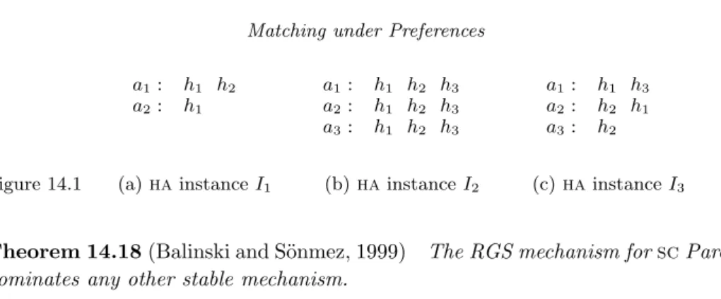
a1: h1 h2 a1: h1 h2 h3 a1: h1 h3 a2: h1 a2: h1 h2 h3 a2: h2 h1
a3: h1 h2 h3 a3: h2
Figure 14.1 (a)ha instanceI1 (b)hainstanceI2 (c)hainstanceI3
Theorem 14.18(Balinski and S¨onmez, 1999) The RGS mechanism forscPareto dominates any other stable mechanism.
Finally, when focusing on strategy-proofness and Pareto optimality only, no bet-ter mechanism than the RGS mechanism emerges.
Theorem 14.19 (Kesten, 2010) The RGS mechanism for sc is not
Pareto-dominated by any other Pareto optimal mechanism that is strategy-proof.
14.3.4 Further algorithmic results Pareto optimal matchings
For a given instance ofha, Pareto optimal matchings may have different sizes, as illustrated by Figure 14.1(a): for the instanceI1shown, matchingsM1={(a1, h1)} andM2={(a1, h2),(a2, h1)}are both Pareto optimal. In many applications we seek to match as many applicants as possible. This motivates the problem of finding a Pareto optimal matching of maximum size, which we refer to as amaximum Pareto optimal matching.
Towards an algorithm for this problem, Abraham et al. (2004) gave a charac-terisation of Pareto optimal matchings in a given ha instance I. A matching M
in I is maximal if there is no pair (ai, hj)∈ E, both of which are unassigned in
M. Also M is trade-in-free if there is no pair (ai, hj) ∈ E such that hj is unas-signed inM, andai is assigned inM and prefershj toM(ai). FinallyM iscyclic
coalition-free if M admits no cyclic coalition, which is a sequence of applicants
C =hai0, ai1, . . . , air−1i, for some r≥ 2, all assigned inM, such that aij prefers
M(aij+1) toM(aij) (0≤j ≤r−1) (with subscripts taken modulo r). Abraham et al. gave the following necessary and sufficient conditions for a matching to be Pareto optimal in terms of these concepts:
Proposition 14.20 (Abraham et al., 2004) Let I be an instance of ha and let
M be a matching in I. Then M is Pareto optimal if and only if M is maximal, trade-in-free and coalition-free. Moreover there is anO(m)algorithm for testingM
for Pareto optimality, wherem is the number of acceptable applicant–house pairs inI.
Abraham et al. also gave a three-phase algorithm for finding a maximum Pareto optimal matching inI, with each phase enforcing one of the conditions for Pareto
optimality given in Proposition 14.20. In Phase 1 they construct a maximum match-ing M in the underlying graph of I, which is the bipartite graph with vertex set
A∪Hand edge setE. This step can be accomplished inO(√n1m) time and ensures that M is maximal. Phase 2 is based on anO(m) algorithm in which assigned ap-plicants repeatedly trade in their own house inM for any preferred vacant house. Once this step terminates, M is trade-in-free. Finally, cyclic coalitions are elim-inated during Phase 3, which is based on an O(m) implementation of the TTC algorithm. Putting these three phases together, they obtained the following result.
Theorem 14.21(Abraham et al., 2004) LetIbe an instance ofha. A maximum Pareto optimal matching in I can be found in O(√n1m) time, where n1 is the
number of applicants andmis the number of acceptable applicant–house pairs inI.
Popular matchings
Pareto optimality is a fundamental solution concept, but on its own it is a rela-tively weak property. A stronger notion is that of apopular matching. Intuitively a matching M in an ha instance I is popular if there is no other matching that is preferred toM by a majority of the applicants who are not indifferent between the two matchings. This concept was first defined by G¨ardenfors (1975) (using the termmajority assignment) in the context ofsmi.
To define the popular matching concept more formally, letM, M0 ∈ M, and let
P(M, M0) denote the set of applicants who prefer M to M0. We say that M0 is
more popular than M, denoted M0 M, if |P(M0, M)| > |P(M, M0)|. Define a matchingM ∈ Mto bepopular (Abraham et al., 2007b) ifM is-maximal (i.e., there is no other matchingM0 ∈ Msuch thatM0M).
Clearly a matchingM is Pareto optimal if there is no other matchingM0 such that|P(M, M0)|= 0 and|P(M0, M)| ≥1. Hence a popular matching is Pareto op-timal. However in contrast to the case for Pareto optimal matchings, anhainstance need not admit a popular matching. To see this, consider thehainstanceI2shown in Figure 14.1(b). It is clear that a matching inI2cannot be popular unless all ap-plicants are assigned. The unique matching up to symmetry in which all apap-plicants are assigned is M = {(ai, hi) : 1 ≤ i ≤ 3}, however M0 = {(a2, h1),(a3, h2)} is preferred by two applicants, which is a majority. The relationin this case cycles, hence the absence of a-maximal solution (therefore, in general,is not a partial order onM).
The potential absence of a popular matching in a given ha instance can be related all the way back to the observation of Condorcet (1785) that, givenkvoters who each rank n candidates in strict order of preference, there may not exist a “winner”, namely a candidate who beats all others in a pairwise majority vote. See also Chapter 2 (Zwicker, 2015).
Abraham et al. (2007b) derived a neat characterisation of popular matchings, leading to anO(m) algorithm to check whether a given matchingM inIis popular.
The same characterisation also led naturally to anO(n+m) algorithm for finding a popular matching or reporting that none exists, wheren=n1+n2. We remark that popular matchings inI can have different sizes, and the authors showed how to extend their algorithm in order to find a maximum popular matching without altering the time complexity. This discussion can be summarised as follows.
Theorem 14.22 (Abraham et al., 2007b) Let I be an instance of ha. There is anO(n+m)algorithm to find a maximum popular matching inI or report that no popular matching exists, wherenis the number of applicants and houses, and mis the number of acceptable applicant–house pairs.
A more complex algorithm, with O(√nm) complexity, can be used to find a maximum popular matching inI or report that no popular matching exists, in the case that preference lists include ties (Abraham et al., 2007b).
McDermid and Irving (2011) showed that the set of popular matchings in an ha instance can be characterised succinctly via a structure known as the
switch-ing graph. Using this representation they showed that a number of problems can be solved efficiently, including counting popular matchings, sampling a popular match-ing uniformly at random, listmatch-ing all popular matchmatch-ings and findmatch-ing various types of “optimal” popular matchings.
As a given ha instance need not admit a popular matching, it is natural to weaken the notion of popularity, and seek matchings that are as popular as possible in cases where a popular matching does not exist. To this end, McCutchen (2008) defined two versions of near-popular matchings, namely aleast unpopularity factor matching and a least unpopularity margin matching. Also Kavitha et al. (2011) studied the concept of apopular mixed matching, which is a probability distribution over matchings that is popular in a precise sense.
Profile-based optimal matchings
Further notions of optimality are based on theprofile p(M) of a matchingM in an hainstance I. Informally,p(M) is anr-tuple whose ith component is the number of applicants who have theirith-choice house, wherer is the maximum length of an applicant’s preference list.
A matchingM isrank-maximal (Irving et al., 2006) if p(M) is lexicographically maximum, taken over all matchings inM. Intuitively, in such a matching, the max-imum number of applicants are assigned to their first-choice house, and subject to this condition, the maximum number of applicants are assigned to their second-choice house, and so on. A rank-maximal matching need not be of maximum cardi-nality. To see this, consider theha instanceI3 in Figure 14.1(c) and the following matchings in I3: M1 = {(a1, h1),(a2, h2)} and M2 = {(a1, h3),(a2, h1),(a3, h2)}. ClearlyM1 is rank-maximal and|M1|= 2, whereas|M2|= 3.
In many applications we seek to assign as many applicants as possible. With this in mind, consider M+, the set of maximum matchings in a given
A greedy maximum matching is a matching M ∈ M+ such that p(M) is lexico-graphically maximum, taken over all matchings in M+. Both rank-maximal and greedy maximum matchings maximise the number of applicants with their s th-choice house as a higher priority than maximising the number of those with their
tth-choice house, for any 1≤s < t≤r. As a consequence, both of these types of matchings could end up assigning applicants to houses relatively low down on their preference lists.
Consequently, define agenerous maximum matching to be a matchingM ∈ M+ such that pR(M) is lexicographically minimum, taken over all matchings in M+, wherepR(M) is the reverse ofp(M). That is,M is a maximum cardinality matching that assigns the minimum number of applicants to their rth-choice house, and subject to this, the minimum number to their (r−1)th-choice house, and so on.
We collectively refer to rank-maximal, greedy maximum and generous maximum matchings as profile-based optimal matchings. Returning to instance I3 shown in Figure 14.1(c), the matching M2 defined above is the unique maximum match-ing and is therefore both a greedy maximum matchmatch-ing and a generous maximum matching.
The following results indicate the complexity of the fastest current algorithms for constructing rank-maximal, greedy maximum and generous maximum matchings in a givenhainstance.
Theorem 14.23(Irving et al., 2006) LetI be an instance ofha. A rank-maximal matching M in I can be constructed inO(min(n1+r∗, r∗
√
n1)m) time, wheren1
is the number of applicants, m is the number of acceptable applicant–house pairs, andr∗ is the maximum rank of an applicant’s house inM.
Theorem 14.24(Huang and Kavitha, 2012) LetIbe an instance ofha. A greedy maximum matchingM inI can be constructed inO(r∗√nmlogn)time, wherenis the number of applicants and houses,mis the number of acceptable applicant–house pairs, and r∗ is the maximum rank of an applicant’s house in M. The same time complexity holds for computing a generous maximum matching.
The algorithms referred to in Theorems 14.23 and 14.24 are also applicable in the more general case that preference list contain ties.
14.4 Concluding remarks and further reading
In this chapter we have tried to cover some of the most important results on match-ing problems with preferences. However the literature in this area is vast, and due to space limitations, we could only cover a subset of the main results in a single survey chapter. Chapter 11 (Thomson, 2015) introduces some of our matching problems within the context of fair resource allocation, namely, object allocation problems
(ha), priority-augmented object allocation problems (sc), and matching agents to each other(smiandhr). The following non-exhaustive list of articles contains nor-mative results for these problems and basic axioms of fair allocation as introduced in Chapter 11 (Thomson, 2015) (e.g., resource-monotonicity, population-monotonicity, consistency, converse consistency): Ehlers and Klaus (2004, 2007, 2011); Ehlers et al. (2002); Ergin (2000); Kesten (2009); Sasaki and Toda (1992); Toda (2006).
One obvious omission has been the Stable Roommates problem (sr), a non-bipartite generalisation ofsm. However a wider class of matching problems, known as hedonic games, which include sr as a special case, are explored in Chapter 15 (Aziz and Savani, 2015).
Looking ahead, it seems likely that the level of interest in matching under pref-erences will show no sign of diminishing, and if anything we predict that this field will continue to grow. This is due in no small part to the exposure that the research area has had on a global stage following the award of the Nobel Prize in Economic Sciences to Alvin Roth and Lloyd Shapley in 2012. Another contributing factor is the increasing engagement by more and more elements of society in forms of electronic communication, thereby easing preference elicitation and centralisation of allocation processes.
To conclude, we give some sources for further reading. For more details on struc-tural and algorithmic aspects ofsm,hrandsr, we recommend Gusfield and Irving (1989). The second author’s monograph (Manlove, 2013) provides an update to Gusfield and Irving (1989) and also expands the coverage to includeha. It expands on the algorithmic results presented in this chapter in particular. For more depth from an economic and game-theoretic viewpoint, the reader is referred to Roth and Sotomayor (1990), which considers issues of strategy insmand hr in much more detail, and also covers monetary transfer and the Assignment Game. Finally, more recent results that also include economic applications (e.g., school choice and kidney exchange) are reviewed by S¨onmez and ¨Unver (2011) and Vulkan et al. (2013).
Acknowledgements
Bettina Klaus acknowledges financial support from the Swiss National Science Foundation (SNFS). David Manlove is supported by grant EP/K010042/1 from the Engineering and Physical Sciences Research Council. Francesca Rossi is partially supported by the project “KIDNEY - Incorporating patients preferences in kidney transplant decision protocol”, funded by the University of Padova. The authors would like to thank Peter Bir´o, Felix Brandt, Vincent Conitzer and Ulle Endriss for detailed comments, which have helped us to improve the presentation of this chapter.