Luminosity functions and galaxy bias in the Sloan Digital Sky Survey

(1)

Luminosity Functions and Galaxy Bias in the

Sloan Digital Sky Survey

by

James G. Cresswell

This thesis is submitted in partial fulfilment of the requirements for the award of the degree of

Doctor of Philosophy of the

University of Portsmouth

(2)

Copyright

c

The copyright of this thesis rests with the Author. Copies (by any means) either in full, or of extracts, may not be made without the prior written consent from the Author.

(3)

This work is dedicated to my parents, without whom I would never have come this far. Thank you.

(4)

Whilst registered as a candidate for the above degree, I have not been registered for any other research award. The results and conclusions embodied in this thesis are the work of the named candidate and have not been submitted for any other academic award.

(5)

Abstract

With the wealth of data provided by modern imaging and redshift surveys, it has be-come essential to obtain measurements of galaxy properties in an automated fashion, and analyse them in a statistical manner.

In this thesis we focus on two fundamental characteristics of the galaxy populations, their distributions in luminosity and their spatial clustering signal .

We examine galaxies from the SDSS-II galaxy redshift survey, quantifying their dis-tribution in luminosity as a function of rest-frame colour and visual morphology taken from the Galaxy Zoo project. In forming samples of the galaxies selected by colour, morphology and luminosity we observe that there are significant populations of both red spiral galaxies and blue early-type galaxies at redshifts of 0.01<z< 0.2.

To aid us in the description and analysis of these distributions we fit them with a para-metric model, the well known Schechter function, in which we include parameterisations for the redshift evolution of absolute magnitude and number density. In comparing the results of fitting our various samples with the function we find that blue galaxies exhibit significantly different behaviour to spiral galaxies and that red galaxies exhibit signifi-cantly different behaviour to early-type galaxies.

We then go on to measure the 2-point clustering statistics of the galaxies in order to explore the dependence of galaxy clustering bias on luminosity and colour. We fit our measurements of scale dependent galaxy clustering with several phenomenological models of galaxy bias. This allows us to describe how the large-scale bias and the transi-tion to non-linear clustering behaviour depend on luminosity and colour. Our key result from this investigation is that red and blue galaxies exhibit significantly different clus-tering behaviour in both the amplitude of their large scale bias and their non-linear bias contributions at smaller scales.

In conclusion we find that in order to extract the maximum amount of cosmological information from future surveys they must be planned and analysed with the understand-ing that galaxy clusterunderstand-ing depends strongly on both luminosity and colour, and that galaxy morphology contains considerable information about a galaxies formation history, inde-pendent of its colour.

(6)

Preface

The work of this thesis was carried out at the Institute of Cosmology and Gravitation University of Portsmouth, United Kingdom.

I would like to take this opportunity to thank my friends for their part in the circumstances which have lead to the writing of this thesis. They have all helped in one way or another, and I would never have made it so far down life’s pathways, at least some of the stranger ones, without them. I don’t have space to thank everyone here, anyone who feels left out should come and buy me a drink so we can talk about it. Alex: you showed me what people could make of themselves if they are determined, and how they can overcome obstacles, and made me want to own chickens. Andre and Susan: without you I would quite clearly have not been here at all, you have both inspired me in many ways, many times. Anna: thank you for so many things, including teaching me the many fine uses of question tags? Oh happy happy tags. Antonio: I am lucky enough to have people in my life who set me good examples, you have set some of the best. Ben: I can’t think of another man I’d rather share a tiny office with for a year. Bjoern: your conscientious-ness and humility in your work is a shining example. You also make excellent gla¨uwine. Chris, Bronwyn and Unknown: Chris, growing up without you around would have been boring, although I might have gotten more sunlight. Diplomat. Bronwyn, I promise not to dig fire pits in your garden without asking first. Unknown, do not trust your father if he tells you to close your eyes and open your hands. Dana¨e: thank you for showing me so clearly what life can be, and for making me want to live up to my potential. Daria: anyone who is lucky enough to have known you will agree that their lives are better and possibly stranger for it. Fabio: writing with you is one of the most enjoyable things I have ever done. We really ought to finish something one of these days. Gaby: mongolita, thank you for encouraging me in my PhD and thesis, in my writing career, and in my gravies; and for being there to listen to me. Good times are here! Condensation. Hidi and Emi: my dear club members, I shall never, ever get bored of watching the film with you, or of drinking fruit juice and checking things. Iain: dude, if it wasn’t for you I might

(7)

never have ended up going to be a middle aged man taking surfing lessons. When the time comes I’ll buy you a beer and you can tell me what I was doing wrong. Jo: I would never have watched all that Doctor Who if it wasn’t for you, you were there whether you were there or not.Kath: I certainly wouldn’t have been doing this if not for you. Thank you. Kelly and Jen: thanks for being such good friends and for being their through the some of the weirder times, it wouldn’t have been the same without you - for one thing it wouldn’t have been as weird. Pudding. Kt: your enthusiasm is contagious, never lose it. We’ve got dancin’ to do. Llin: obviously the whole point of this is that you will have to call me doctor too. Marie: if I am ever half as good at science as you then I will be grateful. Keep it up! Mehri & co.: thank you for for having the strength to remind me that science is only one way of looking at things. Paul: thanks for being there whenever it really counts. I’m really glad I know you. Pete L: I’ve never eaten so much pizza as we did that weekend. I never will again. Thanks for being brilliant. Pete K: you always thought I could understand how the Universe works, I might not have started this other-wise. Thanks! Oli: I have no idea what life would be like without you out there - and no interest in knowing. I think we can almost speak about life with authority at this point, we’d better step up the experiencing of experiences. Sophie: Thank you. For being there, for not being there when I had to work, for anything in between being there and not that you may have been doing. Thank you very, very much.

I would like to thank my PhD supervisor for many useful discussions during the course of my PhD. I would also like to thank my masters degree supervisor, Andrew Liddle, for his support and enthusiasm.

(8)

Acknowledgements

Work in sections 4 and 5 was performed with Steven Bamford and WIll Percival and will be written up and submitted in paper form to MNRAS. The work in section 6 and 7 has been published as “Scale Dependent Galaxy Bias in the SDSS as a Function of Luminosity and Colour” MNRAS 392 682. 2009.

Funding for the SDSS and SDSS-II has been provided by the Alfred P. Sloan Foun-dation, the Participating Institutions, the National Science FounFoun-dation, the U.S. Depart-ment of Energy, the National Aeronautics and Space Administration, the Japanese Mon-bukagakusho, the Max Planck Society, and the Higher Education Funding Council for England. The SDSS Web Site is http://www.sdss.org/. The SDSS is managed by the Astrophysical Research Consortium for the Participating Institutions. The Participating Institutions are the American Museum of Natural History, Astrophysical Institute Pots-dam, University of Basel, University of Cambridge, Case Western Reserve University, University of Chicago, Drexel University, Fermilab, the Institute for Advanced Study, the Japan Participation Group, Johns Hopkins University, the Joint Institute for Nuclear Astrophysics, the Kavli Institute for Particle Astrophysics and Cosmology, the Korean Scientist Group, the Chinese Academy of Sciences (LAMOST), Los Alamos National Laboratory, the Max-Planck-Institute for Astronomy (MPIA), the Max-Planck-Institute for Astrophysics (MPA), New Mexico State University, Ohio State University, University of Pittsburgh, University of Portsmouth, Princeton University, the United States Naval Observatory, and the University of Washington.

This publication has been made possible by the participation of more than 160000 volunteers in the Galaxy Zoo project. Their contributions are individually acknowledged at http://www.galaxyzoo.org/Volunteers.aspx

(9)

List of Tables

1.1 Best fitΛCDM cosmological model key parameters from theLarson et al.

(2010) analysis of the WMAP seven year data. . . 9 2.1 Description of the subcatalogues analysed Chapter 5. The limits of the

absolute magnitude bins are given, with the weighted mean and standard deviation. We also give the galaxy count for each bin. . . 33 3.1 Results of the evolution-corrected Schechter function fits to the r-band

luminosity function for each of our galaxy samples. M⋆_,_α_{and ¯n are the} usual Schechter function parameters, while P and Q are the number den-sity and luminoden-sity evolution parameters. χ2

r is the reduced chi-squared statistic, which provides an estimate of the goodness of the Schechter function fit to the data. A positive value of Q indicates that members of that sample were brighter in the past. A positive value of P indicates that members of that sample were more numerous in the past at a given evolved luminosity (as described by Q). Positive and negative values are coloured orange and green, respectively, for easier viewing. . . 60 4.1 Results of the evolution-corrected Schechter function fits to the r-band

luminosity function for the red and blue galaxy samples defined in Ta-ble2.1. M⋆_,_α_{, P and Q are the Schechter function parameters in Eqn.}_3.5_.

. . . 74 5.1 Maximum Likelihood parameters calculated by fitting the Q-model and

P-model for scale-dependent galaxy bias as given in Eqns. 4.7&4.8, to power spectra calculated for the catalogues described in Table2.1. Best-fit values are presented together with 1-σuncertainties. . . 104 B.1 Correlation matrix of the best fit luminosity function parameters

esti-mated using jackknife resampling for all galaxies. . . 128 B.2 Correlation matrix of the best fit luminosity function parameters

esti-mated using jackknife resampling for red galaxies. . . 128

(13)

B.3 Correlation matrix of the best fit luminosity function parameters esti-mated using jackknife resampling for blue galaxies. . . 128 B.4 Correlation matrix of the best fit luminosity function parameters

esti-mated using jackknife resampling for early-type galaxies. . . 129 B.5 Correlation matrix of the best fit luminosity function parameters

esti-mated using jackknife resampling for spiral galaxies. . . 129 B.6 Correlation matrix of the best fit luminosity function parameters

esti-mated using jackknife resampling for red early-type galaxies. . . 129 B.7 Correlation matrix of the best fit luminosity function parameters

esti-mated using jackknife resampling for blue early-type galaxies. . . 129 B.8 Correlation matrix of the best fit luminosity function parameters

esti-mated using jackknife resampling for red spiral galaxies. . . 129 B.9 Correlation matrix of the best fit luminosity function parameters

(14)

List of Figures

1.1 An illustration of type Ia supernovae discovered in the SDSS-II survey. Each image is centered on a supernova that can be seen with its host galaxy in the background. Credit for image: B. Dilday and the Sloan Digital Sky Survey (http://www.sdss.org). . . 7 1.2 A breakdown of the energy content of the Universe from WMAP 3 data.

Image credit: NASA/the WMAP science team. . . 8 1.3 A Hubble classification tuning fork diagram with thanks to ESA and

NASA for making this diagram publicly available. . . 11 1.4 Illustration of the distribution of galaxies in a slice through the SDSS

galaxy catalouge. Red points represent galaxies with older star popula-tions, blue and green points represent galaxies with younger star popu-lations. Credit for image: M. Blanton and the Sloan Digital Sky Survey (http://www.sdss.org). . . 14 1.5 An example of the effect of bias correction on a power spectrum taken

from taken from Percival et al. (2004). In the upper panel the lower solid thin line shows a standard model power spectrum (dimensionless and ratioed to the power spectrum of the input random catalogue), the upper solid thick line shows the power spectrum corrected for the effect of luminosity dependent bias, the points are data from the 2dFGRS. The lower panel shows the ratio of the two lines, illustrating the effect of not correcting for luminosity dependent bias as a function of scale. . . 19 2.1 The angular mask of the SDSS DR5 main galaxy sample used in the

galaxy zoo morphology analyses. . . 25 2.2 Matched SDSS objects that appear in both the SDSS DR5 and the final

release of the 2dFGRS, positions taken from SDSS. . . 27 2.3 As2.2but for a smaller section with the aspect ratio preserved. Note the

holes in the data, this is caused by unobserved spectroscopic plates in the SDSS data set. . . 27

(15)

2.4 The distribution of a random 10% sample of galaxies in absolute magnitude– redshift space for the SDSS main galaxy sample. Red galaxies are shown in the top panel, blue galaxies in the lower panel. The horizontal, dashed lines denote the boundaries of the absolute magnitude bins. . . 29 2.5 The distribution of galaxies in colour-absolute magnitude space. The

dashed line denotes the boundary of our colour split at M0.1g−M0.1r =0.8. 30

2.6 The distribution of galaxies per absolute magnitude bin as a function of

Mg−Mrcolour. The dashed line denotes the boundary of our colour split

at M0.1g −M0.1r = 0.8. . . 32

2.7 The distribution of a 5% subsample of red galaxies in absolute magnitude– redshift space for the Galaxy Zoo sample. The sample is broken down into red early-type galaxies and red spiral galaxies. The dashed line de-notes the absolute magnitude limit used in the luminosity function fitting. 35 2.8 The distribution of a 5% subsample of blue galaxies in absolute magnitude–

redshift space for the Galaxy Zoo sample. The sample is broken down into blue early-type galaxies and blue spiral galaxies. The dashed line denotes the absolute magnitude limit used in the luminosity function fit-ting. . . 36 2.9 The distribution of a 5% subsample of early-type galaxies in absolute

magnitude–redshift space for the Galaxy Zoo sample. The sample is broken down into red early-type galaxies and blue early-type. The dashed line denotes the absolute magnitude limit used in the luminosity function fitting. . . 38 2.10 The distribution of a 5% subsample of spiral galaxies in absolute magnitude–

redshift space for the Galaxy Zoo sample. The sample is broken down into red spiral galaxies and blue spiral galaxies. The dashed line denotes the absolute magnitude limit used in the luminosity function fitting. . . . 39 2.11 The distribution of red galaxies in redshift for the GalaxyZoo sample.

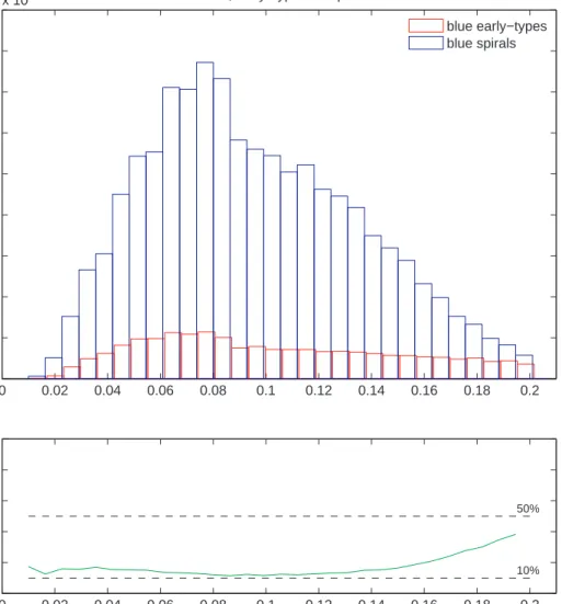
The sample is broken down into red early-type galaxies and red spiral galaxies. Note that within the sample there are never less than_≈ 10% of red galaxies that are spiral. . . 40 2.12 The distribution of blue galaxies in redshift for the GalaxyZoo sample.

The sample is broken down into blue early-type galaxies and blue spiral galaxies. Note that within the sample there are never less than 10% of blue galaxies that are early-type. . . 41 3.1 An illustration of the effect of the Q redshift evolution parameter on a

Schechter luminosity function model at a redshift of z = 0. This can be interpreted as change to the M⋆parameter. . . 48

(16)

3.2 An illustration of the effect of the P redshift evolution parameter on a Schechter luminosity function model at a redshift of z = 0. This can be interpreted as a change in the normalisation of the model. . . 49 3.3 Example SOG fit, large 1/Vmax galaxies causing upturn in faint tail. . . 52

3.4 A proof of good fit for the SOG fits. The initial starting points for the fits, shown by the lines, were randomised. The points represent 1/VMAX

estimates of the luminosity function. The divergence of the two measure-ment techniques at the data-poor faint end of the slope is responsible for the apparent discrepancy in results. . . 53 3.5 An example of the integration limits used in the calculation of the

lumi-nosity functions. The solid green and red lines shows the faint and bright apparent magnitude limits of the survey in absolute magnitude respec-tively. The dashed green and red lines show absolute magnitude limits imposed on the sample by cuts in the data. The curves described by the empty circles show the upper and lower integration limits used in the calculation of the luminosity functions. . . 56 3.6 A Schechter function fit. Note how the 1/Vmax approximation

overesti-mates the luminosity function at both extremes of the distribution, this is a known phenomena (see e.g.Sheth,2007) . . . 58 3.7 A Schechter fit made with a redshift cut at z < 0.01 and an absolute

magnitude cut at0.1Mr >−15.5 is shown by the solid red line. The green

points are the 1/Vmax luminosity function estimate for this data. . . 59 3.8 Average k-correction for all binned in redshift. An interpolation of this

distribution was used in the calculation of integration limits described by Eqn.2.2. . . 61

(17)

3.9 The lower panel shows the luminosity functions for our samples of all (black circles and solid line), red (orange squares and dotted line), blue (cyan triangles and dotted line), early-type (purple crosses and dashed line) and spiral (blue stars and dashed line) galaxies. The lines represent the best-fitting, redshift-evolution corrected z = 0.1 Schechter functions (Eq3.5, see text for details) corresponding to each sample (only consid-ering M0.1_r −5 log h < −18). The points indicate the 1/V_max

evolution-corrected estimates of the true luminosity function, evolution-corrected for redshift evolution (to z= 0.1) using the best-fitting parameters from the relevant Schechter function fits. The points are plotted at the mean magnitude of each bin. The upper panel gives the luminosity functions for each subsample ratioed with luminosity function for the full sample, i.e. the fraction of the total population attributable to each subsample as a func-tion of luminosity. In both panels, error bars are only shown where they exceed the size of the points. . . 62 3.10 An illustration of the redshift evolution of the M⋆parameter from

Equa-tion3.5. The circles show the best-fit values for M⋆from a non-evolving Schechter function fit to a number of redshift slices of the main sam-ple. The solid line shows the M⋆ evolution model given by the best fit Q parameter for the entire sample. Note the limited ability of the linear evolution description, Q (z₋z0), to describe the data. . . 64 3.11 The lower panel shows the luminosity functions for our sample of

early-type galaxies (black circles and solid line), and our early-early-type sample divided into red (orange squares and dotted line) and blue (cyan triangles and dashed line) galaxies. The lines represent the best-fitting, redshift-evolution corrected Schechter functions (Eqn. 3.5, see text for details) corresponding to each sample (only considering M0.1_r−5 log h < −18).

The points indicate the 1/Vmax evolution-corrected estimates of the true luminosity function, corrected for redshift evolution (to z = 0.1) using the best-fitting parameters from the relevant Schechter function fits. The points are plotted at the mean magnitude of each bin. The upper panel gives the luminosity functions for the red and blue early-type subsamples ratioed with luminosity function for the full early-type sample, i.e. the fraction of the early-type population attributable to each colour subsam-ple as a function of luminosity. In both panels, error bars are only shown where they exceed the size of the points. . . 66 3.12 This plot shows the same as Fig. 3.11, but now for spirals rather than

(18)

3.13 Number density at M⋆_all= ₋20.34 versus redshift according to our redshift-dependent luminosity function fits to the morphology subsamples and their breakdown by colour considered in this chapter. Each panel shows the result of fitting to a whole sample (solid, black line), along with the behaviour measured for the two subsamples from which it is composed (coloured, dotted and dashed lines). The sum of the behaviours of the subsamples (dot-dashed, black line) is shown for comparison with that inferred from the fit to the samples combined. . . 70 3.14 Number density at M⋆_all= ₋20.34 versus redshift according to our

redshift-dependent luminosity function fits to the morphology subsamples and their breakdown by colour considered in this article. Each panel shows the result of fitting to a whole sample (solid, black line), along with the behaviour measured for the two subsamples from which it is composed (coloured, dotted and dashed lines). The sum of the behaviours of the subsamples (dot-dashed, black line) is shown for comparison with that inferred from the fit to the samples combined. . . 71 3.15 Number density at M⋆

all= −20.34 versus redshift according to our redshift-dependent luminosity function fits to the colour subsamples and their breakdown by morphology considered in this article. Each panel shows the result of fitting to a whole sample (solid, black line), along with the behaviour measured for the two subsamples from which it is composed (coloured, dotted and dashed lines). The sum of the behaviours of the subsamples (dot-dashed, black line) is shown for comparison with that inferred from the fit to the samples combined. . . 72 4.1 The best fit redshift-evolution corrected Schechter functions presented

in Eqn. 3.5, representing the luminosity functions of the red galaxies, shown as the solid red line, and blue galaxies, shown as the dashed blue line, both at a redshift of z = 0.1. The red, vertical crosses and blue, di-agonal crosses represent the 1/Vmax data estimates of the true luminosity

function for red and blue galaxies respectively, redshift evolution cor-rected using the respective best fit parameters for Eqn. 3.5 to a redshift of z= 0.1. Note that this result is not limited to the Galaxy Zoo data set and so goes out to a redshift of z=0.3. . . 75 4.2 An illustration of the effect of the luminosity function redshift evolution

parameter Q on the derived redshift distribution. The black histogram shows the normalised distribution of the data in redshift, the red curve shows a model with Q= ₋3, the black curve shows the same model with

(19)

4.3 An illustration of the effect of the luminosity function redshift evolution parameter P on the derived redshift distribution. The black histogram shows the normalised distribution of the data in redshift. The coloured curves shows the P parameter ranging from P = ₋5 for the reddest line (the top curve for z < 0.1) to P = 5 for the bluest line (the top curve for

z>0.1), the green curve shows a typical best fit result. . . 77 4.4 An illustration of a redshift evolution corrected Schechter function

de-rived redshift distribution compared to the binned redshift counts of the data it was derived from. . . 78 4.5 An example plot where the redshift distribution model is derived from

the distribution of galaxies in absolute magnitude where a contribution is made to each redshift bin that a galaxy could have been observed in, dependent on the survey apparent magnitude limits, and each redshift bin is then weighted by dV/dZ . This qualitatively demonstrates that the

redshift distributions derived from luminosity function fits provide the correct functional form. This analysis assumes no redshift evolution of absolute magnitude. . . 79 4.6 Histogram showing the redshift distribution of galaxies in the absolute

magnitude and colour bins defined in Table2.1. Plots on the left are for blue galaxies, plots on the right are for red galaxies. Top to bottom the plots represent magnitude bins 1 (-22.30 _≤ M0.1r < -21.35), 2 (-21.35

≤ M0.1r < -20.89) and 3 (-20.89 ≤ M0.1r < -20.47) respectively. The

black is the binned redshift distribution of the data, the cyan line is the model distribution derived from the appropriate luminosity function via the relation shown in Eq. 4.1) calculated at each bin centre, the red line is the monte-carlo sampled redshift distribution drawn from the model. . 81 4.7 Histogram showing the redshift distribution of galaxies in the absolute

magnitude and colour bins defined in Table2.1. Plots on the left are for blue galaxies, plots on the right are for red galaxies. Top to bottom the plots represent magnitude bins 4 (-20.47 _≤ M0.1r < -20.00), 5 (-20.00

≤ M0.1r < -19.34) and 6 (-19.34 ≤ M0.1r < -17.00) respectively. The

black is the binned redshift distribution of the data, the cyan line is the model distribution derived from the appropriate luminosity function via the relation shown in Eq. 4.1) calculated at each bin centre, the red line is the monte-carlo sampled redshift distribution drawn from the model. . 82

(20)

4.8 Expected comoving number density as a function of redshift. Plots on the left are for blue galaxies, plots on the right are for red galaxies. Top to bottom the plots represent magnitude bins 1, 2 and 3 respectively. The empty circles show the model predictions for comoving number den-sity derived from the model redshift distributions for each bin. The red crosses show data estimates of the comoving number density in each red-shift bin for comparison. . . 83 4.9 Expected comoving number density as a function of redshift. Plots on

the left are for blue galaxies, plots on the right are for red galaxies. Top to bottom the plots represent magnitude bins 4, 5 and 6 respectively. The empty circles show the model predictions for comoving number den-sity derived from the model redshift distributions for each bin. The red crosses show data estimates of the comoving number density in each red-shift bin for comparison. . . 84 4.10 Comparison of data and mock power spectra in each of the absolute

mag-nitude bins for red galaxies described in Table. 2.1. The data power spectra shown by the solid lines were created using the method given in Section.4.3. Mock catalogues were created using the methods given in Section 4.4 and spectra generated the same way, the dot-dash lines here show the average mock power spectrum for each sample. . . 86 4.11 Comparison of data and mock power spectra in each of the absolute

mag-nitude bins for blue galaxies described in Table. 2.1. The data power spectra shown by the solid lines were created using the method given in Section.4.3. Mock catalogues were created using the methods given in Section4.4 and spectra generated the same way, the dot-dash lines here show the average mock power spectrum for each sample. . . 87 4.12 Examples of measured power spectra with estimated uncertainties for the

brightest red bin and faintest blue bin. . . 88 4.13 Comparison of data and linear theory dark matter power spectra in each

of the absolute magnitude bins for red galaxies described in Table. 2.1. The data power spectra shown by the solid lines were created using the method given in Section.4.3. The dark matter linear theory power spectra shown by the dotted lines we generated as set out in Section4.5, each was convolved with the window function of the appropriate galaxy sample. . 90

(21)

4.14 Comparison of data and linear theory dark matter power spectra in each of the absolute magnitude bins for blue galaxies described in Table.2.1. The data power spectra shown by the solid lines were created using the method given in Section.4.3. The dark matter linear theory power spectra shown by the dotted lines we generated as set out in Section4.5, each was convolved with the window function of the appropriate galaxy sample. . . 91 4.15 Example comparison of the fiducial, linear theory power spectrum model

for the brightest red bin multiplied by the best fit results for the Q-model (solid, red line), and P-model (dashed, brown line). . . 93 4.16 The variation of the Q-model shape as Q varies with a fixed large scale

bias parameter. The large scale bias is kept fixed at the best fit Q-model parameter value for the brightest red bin, the input linear spectrum is for the same colour-magnitude bin, Q varies as shown in the legend. The black line shows the best fit parameter model for same colour-magnitude bin. . . 94 4.17 The variation of the P-model shape as P varies with a fixed large scale

bias parameter. The large scale bias is kept fixed at the best fit P-model parameter value for the brightest red bin, the input linear spectrum is for the same colour-magnitude bin, Q varies as shown in the legend. The black line shows the best fit parameter model for same colour-magnitude bin. . . 95 5.1 Comparison of relative, large-scale, constant, linear bias as a function

of luminosity for galaxies split into red and blue colours. Five and six pointed stars represent our measurements of bias relative to our red galaxy

M⋆bin, for red and blue galaxies respectively. The horizontal dashed line shows no bias relative to our red M⋆bin. . . 100 5.2 As Fig. 5.1additionally with the upper, solid line is a fit to Eq.4.11 for

our red galaxy bias points, see text for details. The lower, dash-dot line is the fit to blue galaxies. . . 101 5.3 As Fig.5.1additionally with squares and circles showing the results from

Swanson et al.(2008) renormalised to match our M⋆values, see text for

details. . . 102 5.4 Comparison of best-fit power spectra calculated with bias from the

Q-model (solid lines) to the data (circles with 1σerrors). The power spec-trum for each sample (see Table 2.1) is divided by our fiducial linear power spectrum convolved with the appropriate window function. . . 105 5.5 As Fig. 5.4 (see Table 2.1 for sample descriptions), but now for model

(22)

5.6 Best-fit blinmodel parameter as a function of absolute magnitude, as

pre-sented in Table5.1, from a fit including the Q-model bias prescription. Circles and crosses are for red and blue galaxies respectively. Solid, hor-izontal lines about each data point show the extent of each absolute mag-nitude bin. The solid line shows the model of Eqn.5.1and the dashed line shows the model of 5.2 red and blue galaxies respectively. It should be noted that the models were not fitted to the individual data points above but rather to all galaxy bias measurements in a given colour bin simulta-neously, and so the lines representing the magnitude dependence of the individual model parameters are here shown only for comparison. . . 109 5.7 Best-fit Q model parameter as a function of absolute magnitude, as

pre-sented in Table5.1, from a fit including the Q-model bias prescription. Circles and crosses are for red and blue galaxies respectively. Solid, hor-izontal lines about each data point show the extent of each absolute mag-nitude bin. The solid line shows the model of Eqn.5.1and the dashed line shows the model of 5.2for red and blue galaxies respectively. It should be noted that the models were not fitted to the individual data points above but rather to all galaxy bias measurements in a given colour bin simultaneously, and so the lines representing the magnitude dependence of the individual model parameters are here shown only for comparison. . 110 5.8 Best-fit blinmodel parameter as a function of absolute magnitude, as

pre-sented in Table 5.1, from a fit including the P-model bias prescription. Circles and crosses are for red and blue galaxies respectively. Solid, hor-izontal lines about each data point show the extent of each absolute mag-nitude bin. The solid line shows the model of Eqn.5.1and the dashed line shows the model of 5.2for red and blue galaxies respectively. It should be noted that the models were not fitted to the individual data points above but rather to all galaxy bias measurements in a given colour bin simultaneously, and so the lines representing the magnitude dependence of the individual model parameters are here shown only for comparison. . 111

(23)

5.9 Best-fit P model parameter as a function of absolute magnitude, as pre-sented in Table 5.1, from a fit including the P-model bias prescription. Circles and crosses are for red and blue galaxies respectively. Solid, hor-izontal lines about each data point show the extent of each absolute mag-nitude bin. The solid line shows the model of Eqn.5.1and the dashed line shows the model of 5.2for red and blue galaxies respectively. It should be noted that the models were not fitted to the individual data points above but rather to all galaxy bias measurements in a given colour bin simultaneously, and so the lines representing the magnitude dependence of the individual model parameters are here shown only for comparison. . 112 5.10 As Fig.5.4, but now showing models with parameters calculated from a

simple fit to the luminosity dependent trends observed in Figs.5.6,5.7,5.8&5.9. 113

5.11 As Fig.5.5, but now showing models with parameters calculated from

our simple fit to the luminosity dependent trends observed in Figs.5.6,5.7,5.8&5.9. 115

B.1 The scatter in the best-fit Q and P luminosity function parameters for the jackknife resamplings of the galaxies. . . 126 B.2 The scatter in the best-fit Q and P luminosity function parameters for the

jackknife resamplings of the galaxies. . . 127 C.1 The distribution of galaxies per absolute magnitude bin as a function of

Mg−Mrcolour. The dashed line denotes the boundary of the colour split

at M0.1g−M0.1r =0.8. The dot-dash line denotes the magnitude dependent

colour split calculated as an investigation of the validity of the original split. . . 132 C.2 The distribution of galaxies in colour-absolute magnitude space. The

dashed line denotes the boundary of the colour split at M0.1g−M0.1r = 0.8.

The dot-dash line denotes the magnitude dependent colour split calcu-lated as an investigation of the validity of the original split. . . 133 C.3 Luminosity functions fits for the red galaxy sample. The lines represent

the best-fitting, redshift-evolution corrected z = 0.1 Schechter functions (Eq3.5, the solid line corresponds to the constant colour cut used in the main text, the dashed line corresponds to the magnitude dependent colour cut. The points indicate the 1/Vmax-corrected estimates of the true lumi-nosity function, corrected for redshift evolution (to z = 0.1) using the best-fitting parameters from the relevant Schechter function fits,+ sym-bols represent the result for the constant cut and squares the magnitude dependent cut. The points are plotted at the mean magnitude of each bin. . 134

(24)

C.4 Luminosity functions fits for the blue galaxy sample. The lines represent the best-fitting, redshift-evolution corrected z = 0.1 Schechter functions (Eq3.5, the solid line corresponds to the constant colour cut used in the main text, the dashed line corresponds to the magnitude dependent colour cut. The points indicate the 1/Vmax-corrected estimates of the true lumi-nosity function, corrected for redshift evolution (to z = 0.1) using the best-fitting parameters from the relevant Schechter function fits,+ sym-bols represent the result for the constant cut and squares the magnitude dependent cut. The points are plotted at the mean magnitude of each bin. . 135 C.5 Luminosity functions fits for the red early-type and blue early-type galaxy

sample. The lines represent the best-fitting, redshift-evolution corrected

z = 0.1 Schechter functions (Eq 3.5, the red dot and blue dash-dot lines corresponds red and blue early-type results using the constant colour cut used in the main text, the red dotted and blue dotted lines cor-responds red and blue early-type results using the magnitude dependent colour cut. The points indicate the 1/Vmax-corrected estimates of the true luminosity function, corrected for redshift evolution (to z = 0.1) using the best-fitting parameters from the relevant Schechter function fits, cross symbols represent the result for the constant cut and circles the magni-tude dependent cut. The points are plotted at the mean magnimagni-tude of each bin. . . 136 C.6 Luminosity functions fits for the red spiral and blue spiral galaxy sample.

The lines represent the best-fitting, redshift-evolution corrected z = 0.1 Schechter functions (Eq3.5, the red dash-dot and blue dash-dot lines cor-responds red and blue spiral results using the constant colour cut used in the main text, the red dotted and blue dotted lines corresponds red and blue spiral results using the magnitude dependent colour cut. The points indicate the 1/Vmax-corrected estimates of the true luminosity function, corrected for redshift evolution (to z = 0.1) using the best-fitting param-eters from the relevant Schechter function fits, cross symbols represent the result for the constant cut and circles the magnitude dependent cut. The points are plotted at the mean magnitude of each bin. . . 137

(25)

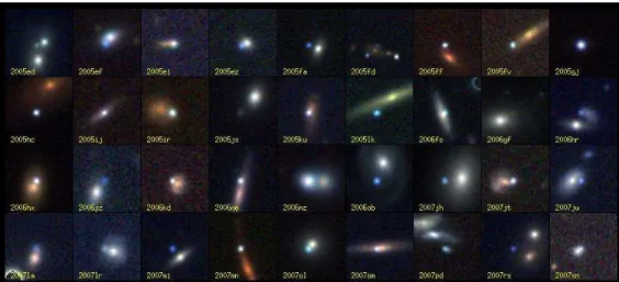
D.1 A random selection from our blue spirals sample, with z_≈ 0.05 and ab-solute magnitude close to the mean of our whole sample at that redshift,

M0.1_r ≈ −19.4. The images are ordered by their colour and morphology,

such that objects which only just satisfy the criteria for this sample are at top-left, whereas those which have very blue colour and high psp are at bottom-right. The numbers by each object give their pspand their true

M0.1_g− M0.1_rcolour, respectively. . . 139

D.2 As Fig.D.1, but for blue early-types. . . 140 D.3 As Fig.D.1, but for red spirals. . . 140 D.4 As Fig.D.1, but for red early-types. . . 141 D.5 A random selection from our blue spirals sample, with z_≈ 0.10 and

ab-solute magnitude close to the mean of our whole sample at that redshift,

M0.1_r≈ −20.5. Other details as for Fig.D.1. . . 141

D.6 As Fig.D.5, but for blue early-types. . . 142 D.7 As Fig.D.5, but for red spirals. . . 142 D.8 As Fig.D.5, but for red early-types. . . 143 D.9 A random selection from our blue spirals sample, with z_≈ 0.15 and

ab-solute magnitude close to the mean of our whole sample at that redshift,

M0.1_r≈ −21.2. Other details as for Fig.D.1. . . 143

D.10 As Fig.D.9, but for blue early-types. . . 144 D.11 As Fig.D.9, but for red spirals. . . 144 D.12 As Fig.D.9, but for red early-types. . . 145

(26)

Chapter 1 Introduction

Cosmology is the study of the past and future evolution the physical Universe (Peebles,

1994;Liddle, 2003;Peacock, 2003). In this chapter we work from the basic principles

up to the current observation and theory, setting the scene for the rest of the work that will be presented in this thesis to take the field forward.

We first review General Relativity, the cosmological framework describing the re-lationship between mass-energy and the geometry of space-time, in which the analyses presented in this thesis will be carried out. A key observable in understanding the distri-bution of mass in the Universe is the recession velocity of objects, related to their distance from us and measured via their redshift which is introduced in Section1.2. We then con-sider how this distribution of baryonic matter is clumped into high density regions called galaxies which themselves have a non-random clustering signal. We introduce the con-cept of measuring the distribution of galaxies in terms of their light output or luminosity. We then discuss the relationship between the clustering of the galaxies and the distribu-tion of the total mass, a reladistribu-tionship referred to as galaxy bias. In this thesis we use the dependence of the luminosity distributions and galaxy bias on other observable galaxy properties to constrain relationships between different galaxy populations, an overview of the new work is given in Section1.10.

1.1 The standard cosmological model

The standard description of the evolution of Universe on the largest scales is derived from Einstein’s General Relativity and assumes a Hot Big Bang event followed by a period of inflation.

(27)

CHAPTER 1. INTRODUCTION 2

1.1.1 Einstein’s theory of general relativity

The Einstein equations, relating the mass-energy content of the Universe to the geometry of space-time, with a geometrical cosmological constant, are:

Gµν−Λgµν= 8πG

c4 Tµν. (1.1)

Assuming the validity of the Cosmological Principle, which states that the Universe is homogeneous and isotropic, the Friedmann-Lemaˆıtre-Roberston-Walker time-dependent solution may be derived:

c2dτ2 =c2dt2₋a(t)2 dr 2 1₋kr2 +r 2_d_θ2₊_r2_sin2 θdφ2 ! , (1.2)

where a(t) is the scale factor of the Universe, normalised to unity in the present (a(t0)= 1) and k indicates the intrinsic curvature of space-time taking one of three values

k=₋1,0,+1, corresponding to negative, zero and positive curvature respectively. From this solution it is possible to derive the dependence of the scale factor evolution on the mass-energy content of the Universe:

H2 = _˙a a 2 = 8πG 3 ρ− kc2 a2 + Λc2 3 , (1.3)

referred to as the Friedmann equation, where ρ is the total energy density of the Universe andΛcan be interpreted as field with an energy density that does not depend on the expansion of the Universe. Defining a critical density of the Universe which satisfies the condition k=0 we have:

ρc =

3H2

8πG, (1.4)

which we may use to rewrite the Friedmann equation in terms of critical densities, e.g.Ω_M = ρM/ρcrit:

H2(a)= H2₀hΩ_DE + Ω_ma−3+ Ω_ra−4₋(Ω₋1) a2i, (1.5) whereΩ_DEis the dark energy density,Ω_mis the non-relativistic matter energy density andΩ_r is the radiation energy density and H0 is defined in Eqn.1.10. From Eqn.1.5it can be seen that different components of the matter-energy content of the Universe dom-inate the evolution at different times, see Section.1.4for more details.

Various alternatives to Einstein gravity and the standard model of cosmology have been proposed. However, to be considered as a replacement theory each must be at least as consistent with current observations as General Relativity. Some examples are:

(28)

CHAPTER 1. INTRODUCTION 3 Self-accelerating models which do not require a cosmological constant, (e.g. Silva &

Koyama,2009); Bouncing cosmologies which do away with the difficult question of why

a big bang scenario might arise (e.g. Cardoso & Wands, 2008) and non-trivial spatial topologies (e.g Cresswell et al., 2006) in which General Relativity still applies to the local geometry, but the usually unspecified global topology is assumed to be non-trivial and non-infinite in at least one direction.

1.2 Redshift

Observed redshift is a ratio of the emission of light from an object at an assumed rest-frame wavelength and at the observed wavelength after Doppler shifting due to the mo-tion of the object away from the observer (Hogg,1999):

z_≡ νe

νo −

1= λo

λe −

1. (1.6)

The radial motion is due to a combination of the expansion of the Universe, referred to as the Hubble flow, and the radial component of the non-cosmological peculiar velocity of the object. Ignoring peculiar velocities, we may write,

1+z= a(t0)

a(te)

= 1

a(te)

. (1.7)

For small redshifts, and hence small distances, d (see Section.1.3), we have,

z_≈ v c =

d DH

, (1.8)

where DHis the Hubble distance defined in Eqn.1.11.

There are two processes which cause an object’s redshift to deviate from the relation described in Eqn.1.8. The first effect is the peculiar velocity of a given galaxy due to the galaxy’s motion towards some local overdensity in the matter field, known as the Kaiser effect this distorts distance measurements inferred from redshifts and so distorts cluster-ing measurements. The second is known as the Fcluster-ingers of God effect, the virialisation of the motion of collapsing objects increasing their velocity dispersion (e.gKaiser, 1987). Efforts can be made to mitigate the effects of these processes, however this introduces a new source of potential systematic error into the analysis and in this thesis we choose to carry out our work in redshift space with an application of the methods of Chapters3&4 to redshift space distortion corrected data left to future work.

(29)

1.3 Distance and volume measurements

Eqn.1.8gives a linear relationship between redshift and distance. If we assume a linear relationship between redshift and recession velocity (which is valid for small z) then it is possible to surmise a linear relationship between recession velocity v and distance d (Hogg,1999):

v= H0d. (1.9)

where H0 is the constant of proportionality. This is also the only recession velocity-distance relationship that satisfies the cosmological principle (Peacock, 2003). This re-lation was confirmed to be a good fit to the available data in one of the earliest result in observational physical cosmology byHubble(1929). A current best estimate of this parameter is 71.0_± 2.5Km.s−1_._{M pc}−1 ₍_{Larson et al.}_, ₂₀₁₀_{), where 1 parsec (pc) is the} distance from a point to an object which subtends 1 arcsecond of parallax angle against a fixed (distant) reference when the observer moves 1 astronomical unit (AU, the mean distance from the Earth to the Sun) perpendicular to the line of sight.

It is common to write the Hubble constant in terms of a dimensionless Hubble pa-rameter (Hogg,1999):

H0 =100 h [km s−1M pc−1]. (1.10) The Hubble distance is a convenient quantity often used to define distance measures:

DH =

c H0

. (1.11)

The luminosity distance is defined as

DL≡ r

L

4πS, (1.12)

where L is the bolometric luminosity and S is the flux.

The angular diameter distance is defined as the ratio of an object’s physical transverse size to its angular extent:

DA(z)=

transverse size

(α) , (1.13)

whereαis the angle subtended by the object ion the sky.

A comoving distance can be defined for which objects that only move relative to each other with the expansion of the Universe always have the same separation, the radial

(30)

CHAPTER 1. INTRODUCTION 5 comoving distance may be written as:

DC(z)= DH Z z 0 dz′ E(z′₎. (1.14) where, E(z)_≡ pΩ_M(1+z)3_{+ Ω} k(1+z)2+ ΩΛ, (1.15) and Ω_M+ Ω_k+ ΩΛ= 1. (1.16)

The luminosity distance, transverse comoving distance and angular diameter distance are related by:

DL(z)=(1+z)DM(z)=(1+z)2DA(z). (1.17)

AssumingΩ_k =0 allows us to write

DM(z)= DC(z). (1.18)

The comoving volume element may then be defined as:

dVc = DH (1+z)2_D2 A E(z) dΩdz= DH D2_C E(z)dΩdz, (1.19)

where dΩis the solid angle element.

1.4 A brief history of the Universe

The observation that the Universe is currently expanding implies that it was smaller in the past; following energy conservation the Universe must have been hotter and denser when it was small, and so these models are called Hot Big Bang models.

In inflationary models (Guth, 1981) the very early universe undergoes a period of exponential expansion. These models conveniently explain the apparent flatness of the Universe in the current epoch and uniformity of the temperature across the cosmic mi-crowave background in areas which would not otherwise have been in causal contact. Density perturbations in the post-inflation Universe are assumed to have been seeded by quantum fluctuations which were blown up by the inflation event (Peacock, 2003). This hot, dense plasma cooled as it expanded. When the average temperature of the plasma reach 13.5eV electrons combined with protons to form neutral helium and the mean free

(31)

CHAPTER 1. INTRODUCTION 6 path of the photons became effectively infinite. The relic radiation from this decoupling has cooled to an average temperature of 2.73 Kelvin due to the expansion of the Universe and is referred to as the cosmic microwave background (CMB) (e.g.Bennett et al.,1996). See Section1.5.3for a brief overview of some of the CMB observational experiments.

From equation1.5 it can be seen that the evolution of the Universe is dominated by different components at different times. At very early times, as a_→0 the radiation term, dependent on the largest inverse power of the scale factor, dominates the dynamics. At late times, as a _{→ ∞}all the terms other than the cosmological constant vanish. As the matter term is dependent on a smaller inverse power of the scale factor than the radiation term, the matter term will dominate at intermediate times.

During the matter dominated era the density perturbations in the matter grow due to gravitational collapse. Baryonic matter forms into gravitationally bound structures, called galaxies, which are described in Section1.6.

1.5 Current cosmological constraints

Astrophysical cosmology, combining truly huge datasets (e.g.Bennett et al., 1996;

Col-less et al., 2003; Adelman-McCarthy et al., 2006;Hinshaw et al., 2007;Spergel et al.,

2007) and the tools of statistical inference (e.g. Lewis & Bridle, 2002; Hobson et al.,

2002; Marshall et al., 2006; Liddle et al., 2006; Lahav & Liddle, 2006), has told us a

huge amount about the nature of the observable Universe. The primary dataset used in this thesis is the Sloan Digital Sky Survey (Adelman-McCarthy et al., 2006); where cosmological parameters are assumed in analyses they are taken from the WMAP exper-iment third year data, best fit WMAP only results (Spergel et al.,2007) unless specified otherwise.

1.5.1 Evidence for the existence dark matter

Since the 1930s observational evidence has been gathered that suggests that the majority of matter in the Universe is not visible. In 1937 measurements of the mass of the Coma galaxy cluster were made based on both the amount of luminous matter visible and the dynamics of galaxies within it from the application of the Virial theorem, the dynamical mass estimate exceeded that of the luminous matter by a factor of_∼ 500 (Zwicky,1937). In 1970 measurements of the rotation curve of the Andromeda galaxy M31 showed devia-tion from simple Keplerian modevia-tion out to a high galactic radius suggesting the presence of unseen matter (Rubin & Ford,1970). There have also been attempts to detect “dark mat-ter” more directly through effects such as gravitational lensing (Kochanek,2005;Clowe

(32)

Figure 1.1: An illustration of type Ia supernovae discovered in the SDSS-II survey. Each image is centered on a supernova that can be seen with its host galaxy in the background. Credit for image: B. Dilday and the Sloan Digital Sky Survey (http://www.sdss.org).

et al.,2006) and interactions with underground detectors (Sumner,2004). For reviews of

astronomical dark matter observational evidence seeRubin(2003);Kuijken(2005).

1.5.2 Evidence for the existence of dark energy

Observations of supernovae have provided evidence that the expansion of the Universe is accelerating (e.g.Perlmutter et al., 1998;Riess et al.,1998; Dilday et al., 2010). Su-pernovae type Ia occur when a white dwarf star reaches its Chandrasekhar mass limit and undergoes a massive amount of nuclear fusion in a short time, _∼ days. After nor-malisation the shape of the emitted light-curve is near identical in all cases, allowing the supernovae to be used as standard candles. This provides direct measurement of the ob-ject’s redshift and luminosity distance. Fitting cosmological models to this distribution favours the existence of a cosmological constant, referred to as a dark-energy field, as seen in Eqns.1.1 &1.3. It has been suggested that dark energy and dark matter might interactCaldera-Cabral et al.(2009).

Figure1.1illustrates a sample of type Ia supernovae taken from the SDSS-II survey. Note how in each case they outshine their host galaxy.

1.5.3 Information from the cosmic microwave background

The Cosmic Background Explorer (COBE) (Bennett et al.,1996) determined that the cos-mic cos-microwave background radiation (CMB), emitted when the primordial plasma of the early universe became cool enough for a phase transition to predominantly neutral hydro-gen to take place, has an emission spectra of an almost perfect black body with deviations

(33)

Figure 1.2: A breakdown of the energy content of the Universe from WMAP 3 data. Image credit: NASA/the WMAP science team.

from its mean temperature 2.725+/- 0.002 Kelvin across the sky at the level of one part in one hundred thousand. The Wilkinson Microwave Anisotropy Probe (WMAP) (Hinshaw

et al., 2007; Spergel et al., 2007) later made statistically significant measurements of

these tiny fluctuations in the temperature (e.g.Bennett et al.,2003) of the early Universe, indicating the presence of perturbations in density which through gravitational collapse grew to form the large scale, gravitationally bound structures (clusters of galaxies) which we see in the Universe today (Straumann, 2006;Eisenstein et al., 2005). The WMAP experiment has now released a seventh year of scientific data and analyses (e.g.Larson

et al.,2010).

A key result from WMAP was a constraint on the relative contribution of the compo-nents of the Universe to the total energy density, see Figure1.2for typical results.

Assuming aΛCDM cosmological model in which the Universe contains energy den-sity contributions from a cosmological constant, cold dark matter and baryonic matter, the current best fit WMAP parameters are given in Table1.1.

Where h is the Hubble parameter defined in Eqn. 1.10, Ω_b is the physical baryon density in terms of the critical density as defined in Eqn.1.4,Ω_DMis the cold dark matter density, ΩΛ is the dark energy density, ∆2_R is the amplitude of the primordial, scalar

perturbations,τis the optical depth of the last scattering surface, nsis the spectral of the

density perturbations,Ω_mis the total mass energy density, t0 is the age of the Universe,

σ8 is the amplitude of the density perturbations, in linear theory, smoothed at a scale of 8h−1M pc and zeqis the redshift of matter-radiation equality.

(34)

CHAPTER 1. INTRODUCTION 9 Table 1.1: Best fit ΛCDM cosmological model key parameters from theLarson et al.

(2010) analysis of the WMAP seven year data.

Parameter Best fit value

h 0.710_±0.025 Ω_b 0.0449_±0.0028 Ω_DM 0.222_±0.026 ΩΛ 0.734±0.029 ∆2 R (2.43±0.11)×10− 9 τ 0.088_±0.015 ns 0.963±0.014 Ω_m 0.266_±0.029 t0 13.75±0.13 Gyr σ8 0.801±0.030 zeq 3196₋+134₁₃₃

Larson et al. (2010) state that none of the models they consider are a statistically

better fits to the available data than the ΛCDM model. The persistent success of this model, being also confirmed by other probes such as galaxy redshift surveys, Lyman-alpha surveys and supernovae surveys, has lead to it being referred to as the concordance cosmology.

1.6 Galaxies

We find that the visible baryonic matter is clumped in objects of about 1011solar masses, which are referred to as galaxies. Galaxies can be subdivided according to various ob-servable quantities, such as the distribution of their luminous matter or their colour. We briefly describe such populations in Section1.6.1, first we define galaxy absolute magni-tude and colour.

Apparent magnitude is a measure of the luminosity of an object relative to some zero-point calibration, as for instance given by the AB magnitude system:

mAB= −2.5 log10( fv)−48.60, (1.20)

where fv is the flux from the object measured in erg.sec−1.cm−2.Hz−1 (Oke, 1971).

(35)

CHAPTER 1. INTRODUCTION 10 distance of 10pc and is related to the observed apparent magnitude, m, through Eqn.1.21:

M= m₋log₁₀ " DL(z) 10 [pc] # −K(z), (1.21) where DLis the luminosity distance as defined in Eqn.1.17and K is the k-correction

which corrects for the fact that objects observed at different redshifts are generally ob-served at different rest-frame wavelengths (Hogg et al.,2002) - i.e. it corrects for the fact that for two objects with identical spectra which exist at different redshifts, observed by an instrument with a (set of) finite-width band-pass filter(s) of a given shape, that filter will sample different parts of the rest-frame spectra of the two objects.

Note that the following relationship holds between absolute luminosity and absolute magnitude: log₁₀ L L⋆ = 1 2.5(M−M ⋆₎ , (1.22)

where L⋆ _{and M}⋆ _{are a reference absolute luminosity and magnitude for the same} source (Lang,1997).

Rest frame colour as used throughout this thesis is defined as the difference between two absolute magnitudes observed through different band-pass filters. Throughout this thesis when we refer to our measurements or analysis of galaxy colour, we specifically mean unless stated otherwise, rest-frame colour defined by the relation:

C = Mg−Mr, (1.23)

where Mg and Mr are the absolute magnitudes observed in the g and r bands of the

Sloan Digital Sky Survey (Fukugita et al.,1996;Gunn et al.,1998) respectively, for more information on the SDSS please see Chapter2.

1.6.1 Galaxy populations

Galaxy morphology and colour have been used as a basis for galaxy population selection (see Sections1.6.2 &1.6.3 for references) although, as there is not a one to one corre-spondence between the two quantities, e.g. not all spiral galaxies are exactly the same colour, it is clear that neither of them uniquely identifies a galaxy’s formation history. Observations of galaxy morphology and colour suggest that there are at least two popula-tions of galaxies with distinct formation histories as discussed in Secpopula-tions1.6.2&1.6.3.

(36)

Figure 1.3: A Hubble classification tuning fork diagram with thanks to ESA and NASA for making this diagram publicly available.

1.6.2 Galaxy morphology

Although a great deal of information about a galaxy’s structure, and so dynamical his-tory, is evident in the distribution of its visible mass, it has proved difficult to extract meaningful quantitative measurements from this morphology; for instance several peo-ple looking at an image of a spiral galaxy could disagree on how many spiral arms it has. Even so, it is clear that the galaxy population can be split into spirals (or late-types) and early-types (comprising elliptical and lenticular galaxies). This natural division strongly implies (at least) two different evolutionary paths. These two broad morphology types and an implied evolutionary history are shown in Figure1.3. Studying the behaviour of these separate morphological classes can help us to understand the physical mechanisms at work in the galaxy population.

In an attempt to include physical, morphological information in studies of large galaxy surveys, a variety of structural statistics have been used as proxies to try to under-stand the importance of different physical processes, and their relationship to large scale physics. The most widespread of these are concentration, the ratio of the radii containing

(37)

CHAPTER 1. INTRODUCTION 12 two different fractions of a galaxy’s total flux (e.g., Strateva et al.,2001); and the index of a Sersic profile fit to a galaxy’s radial profile (e.g.,Blanton et al.,2003c). In principal, concentration and Sersic index quantify the dominance of the spheroid and disk com-ponents within a galaxy. These structural quantities are related to visual morphology, early-type galaxies generally being more concentrated and having higher Sersic indices than spirals; but the correspondence, as with colour, is far from perfect (e.g., van der Wel, 2008), for example these quantities contain no information about spiral arms. Fur-thermore, it has been shown that these quantities display a large scatter versus bulge/disk ratio in a significant fraction of cases, even for model images (Gonzalez et al.,2008).

As part of this thesis we utilise visual morphological classifications for_∼105galaxies from the Galaxy Zoo project (Lintott et al.,2008) to investigate the differences between morphological and colour based divisions of the galaxy population. We do so by measur-ing luminosity functions (see Chapter3), long used as one of the fundamental methods of studying and characterising galaxy populations.

1.6.3 Galaxy colour

The integrated light from a galaxy encodes its star formation history (e.g. Bruzual &

Charlot,2003). Stellar populations of different ages and metallicities in the host galaxy

affect the shape of its observed spectrum (e.g. Bruzual & Charlot, 2003), with older populations resulting in redder spectra with most of the blue light in young populations coming from main sequence stars (e.g.Maraston,1998). The effects of age and metallic-ity on the broadband colours of galaxies are somewhat degenerate (e.g.Maraston,2005;

Renzini,2006).

It has been known for some time that the colour-magntiude relation of early-type galaxies has a predictable form. Given a galaxy with a stellar population of a known metallicity this relationship allows limits to be placed on the age that population (Bower

et al.,1992). Assuming that early-type galaxies tend to be red then this colour-magnitude

relation can be seen in the “red sequence” of Fig.2.5.

Galaxy colour, like galaxy morphology, is observed to be bimodal, again suggesting that there exist at least two observed galaxy populations with different evolutionary his-tories (Strateva et al.,2001;Baldry et al.,2004). In this thesis we are interested in galaxy colour as an empirical selector of galaxy population. It has long been apparent that there is an overall correlation between morphological type and colour, early-types have a ten-dency to be redder red while spirals have a tenten-dency to be more blue. The connection between the morphological structure of a galaxy and its colour has now been shown very clearly (e.g.,Strateva et al., 2001;Driver et al.,2006). Given the simplicity with which

(38)

CHAPTER 1. INTRODUCTION 13 galaxy rest-frame colour can be measured it has become a very popular quantity with which to define galaxy populations for study. Because of this clear correlation it has be-come common practice for studies which utilise colour alone to discuss their results in morphological terms: referring to red galaxies as early-type galaxies and blue galaxies as late-type galaxies. However, this can be misleading, as morphology and colour are certainly not perfectly correlated (e.g. Bernardi et al., 2006) and they provide different and complementary information. Our work investigating the dependence of luminosity functions on both colour and morphology as presented in this thesis is a novel exploration of this relationship.

1.7 Statistical distributions of galaxy properties

Galaxies are not randomly distributed in relation to their observable properties such as absolute luminosity or redshift. A typical galaxy will have an absolute luminosity of ∼1012 solar luminosities and observations show a larger number of small, faint galaxies than large, bright ones.

Luminosity functions are used to describe the distribution of galaxy number number density as a function of absolute luminosity. As stated in Section 1.6.2 we investigate the dependence of luminosity functions on each of galaxy colour and visual morphol-ogy individually and then on both combined. We find non-trivial relationships between colour and morphology, highlighting the need for automated morphological type deter-mination in future survey analysis. For further information on luminosity functions and our methods for measuring and analysing them please see Chapter3.

We then go on to derive redshift and so radial distributions of the galaxies from lu-minosity functions derived for samples selected in colour only. These distributions are subsequently used to measure power spectra for each galaxy sample and so to measure galaxy clustering bias as a function of galaxy colour.

1.8 The distribution of matter in the Universe

The primordial perturbations in the density field grow through gravitational collapse to form over-dense regions in which galaxies form. The angular positions and redshifts of galaxies can then be combined to reveal the three-dimensional distribution of luminous, baryonic matter in the Universe (Peacock,2003;Peebles,1994).