Heuristic decomposition and mathematical programming for workforce scheduling and routing problems

(1)

Laesanklang, Wasakorn (2017) Heuristic decomposition

and mathematical programming for workforce

scheduling and routing problems. PhD thesis, University

of Nottingham.

Access from the University of Nottingham repository: http://eprints.nottingham.ac.uk/39883/1/Wasakorn_Thesis.pdf Copyright and reuse:

The Nottingham ePrints service makes this work by researchers of the University of Nottingham available open access under the following conditions.

This article is made available under the Creative Commons Attribution licence and may be reused according to the conditions of the licence. For more details see:

http://creativecommons.org/licenses/by/2.5/

(2)

School of Computer Science

Heuristic Decomposition and

Mathematical Programming for

Workforce Scheduling and

Routing Problems

Wasakorn Laesanklang

Thesis submitted to the University of Nottingham

for the degree of Doctor of Philosophy

(3)

(4)

Abstract

This thesis presents a PhD research project using a mathematical programming approach to solve a home healthcare problem (HHC) as well as general work-force scheduling and routing problems (WSRPs). In general, the workwork-force scheduling and routing problem consists of producing a schedule for mobile workers to make visits at different locations in order to perform some tasks. In some cases, visits may have time-wise dependencies in which a visit must be made within a time period depending on the other visit. A home healthcare problem is a variant of workforce scheduling and routing problems, which con-sists of producing a daily schedule for nurses or care workers to visit patients at their home. The scheduler must select qualified workers to make visits and route them throughout the time horizon.

We implement a mixed integer programming model to solve the HHC. The model is an adaptation of the WSRP from the literature. However, the MIP solver cannot solve a large-scale real-world problem defined in this model form because the problem requires large amounts of memory and computational time. To tackle the problem, we propose heuristic decomposition approaches which split a main problem into sub-problems heuristically and each sub-problem is solved to optimality by the MIP solver. The first decomposition approach is a geographical decomposition with conflict avoidance (GDCA). The algorithm avoids conflicting assignments by solving sub-problems in a sequence in which worker’s availabilities are updated after a sub-problem is solved. The approach

(5)

can find a feasible solution for every HHC problem instance tackled in this thesis. The second approach is a decomposition with conflict repair and we propose two variants: geographical decomposition with conflict repair (GDCR) and repeated decomposition and conflict repair (RDCR). The GDCR works in the same way as GDCA but instead of solving sub-problems in a given se-quence, they are solved with no specific order and conflicting assignments are allowed. Later on, the conflicting assignments are resolved by a conflict-ing assignments repair process. The remainconflict-ing unassigned visits are allocated by a heuristic assignment algorithm. The second variant, RDCR, tackles the unassigned visits by repeating the decomposition and conflict repair until no further improvement has been found. We also conduct an experiment to use different decomposition rules for RDCR. Based on computational experiments conducted in this thesis, the RDCR is found to be the best of the heuristic de-composition approaches. Therefore, the RDCR is extended to solve a WSRP with time-dependent activities constraints. The approach requires modifica-tion to accommodate the time-dependent activities constraints which means that two visits may have time-wise requirements such as synchronisation, time overlapped, etc.

In addition, we propose a reformulated MIP model to solve the HHC prob-lem. The new model is considered to be a compact model because it has signi-ficantly fewer constraints. The aim of the reformulation is to reduce the solver requirements for memory and computational time. The MIP solver can solve all the HHC instances formulated in a compact model. Most of solutions ob-tained with this approach are the best known solutions so far except for those the instances for which the optimal solution can be found using the full MIP model. Typically, this approach requires computational time below one hour per instance. This problem reformulation is so far the best approach to solve the HHC instances considered in this thesis.

(6)

The heuristic decomposition and model reformulation proposed in this thesis can find solutions to the real-world home healthcare problem. The main achieve-ment is the reduction of computational memory and computational time which are required by the optimisation solver. Our studies show the best way to con-trol the use of solver memory is the heuristic decomposition approach, par-ticularly the RDCR method. The RDCR method can find a solution for every instance used throughout this thesis and keep the memory usage within per-sonal computer memory ranges. Also, the computational time required to solve an instance being less than 8 minutes, for which the solution gap to the optimal solution is on average 12%. In contrast, the strong point of the model reformu-lation approach over the heuristic decomposition is that the model reformula-tion provides higher quality solureformula-tions. The relative gaps of solureformula-tions between the solution for solving the reformulated model and the solution from solving the full model is less than 1% whilst its the computational time could be up to one hour and its computational memory could require up to 100 GB. Therefore, the heuristic decomposition approach is a method for finding a solution us-ing restricted resources while the model reformulation is an approach for when a high solution quality is required. Hence, two mathematical programming based heuristic approaches are each more suitable in different circumstances in which both find high quality solutions within an acceptable time limit.

(7)

(8)

List of Figures

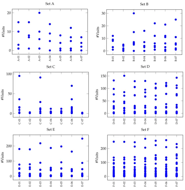
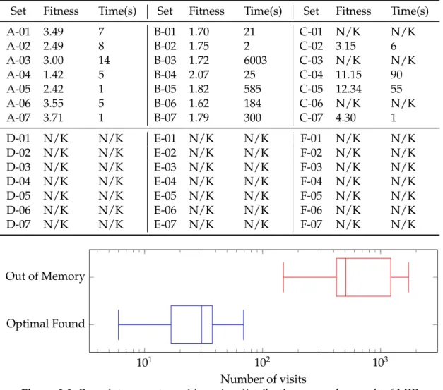
2.1 Distribution of the number of visits in a geographical region of the 42 problem instances . . . 56 2.2 Box plot presents problem size distribution group by result of

MIP solver. . . 58 4.1 Outline of the experimental study in three parts: permutation

study, observation step and strategies study. . . 98 4.2 Relative gap obtained from solving A-04, A-05, A-07 using

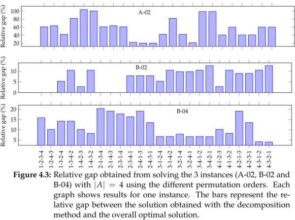
dif-ferent permutation orders. . . 99 4.3 Relative gap obtained from solving A-02, B-02, and B-04 using

different permutation orders . . . 100 4.4 GDCA Computation time used to solve instance sets A, B, D and F105 5.1 Illustrating the Geographical Decomposition with Conflict

Re-pair Approach. . . 113 5.2 Proportion of tasks assigned in the three stages of GDCR. . . 120 5.3 Proportion of travelling distance generated in the three stages of

GDCR. . . 120 5.4 Proportion of computation time used by the three stages of GDCR.121 5.5 Overview of RDCR . . . 123 5.6 Overall results using the nine decomposition procedures within

(15)

5.7 The number of best known solutions and average objective func-tion of automated algorithms and human solufunc-tion . . . 134 6.1 Illustration of the time-dependent constraint modification example

when the assignments do not need the conflicting assignments repair . . . 152 6.2 Illustration of the time-dependent constraint modification example

when the conflicting assignments repair assigns time-dependent activities . . . 154 6.3 Illustration of the time-dependent constraint modification example

when the conflict assignments repair does not assign time-dependent activities . . . 156 6.4 Illustration of the time-dependent constraint modification example

when the conflict assignments repair does not assign one of the time-dependent activities . . . 158 6.5 Number of best solutions obtained by GHI and RDCR . . . 167 6.6 Average relative gap to the best known solution obtained by GHI

and RDCR. . . 167 6.7 Cumulative distribution on relative gap by RDCR and GHI. . . . 169 6.8 Box and Whisker plots showing the distribution of computational

time used by RCDR to solve WSRP . . . 170 7.1 The estimated number of constraints of the full MIP model and

the compact MIP model. . . 197 7.2 Scatter Plot between the number of constraints and the

(16)

List of Tables

2.1 WSRP constraints in the literature . . . 15 2.2 Relation between WSRP conditions/requirements and WSRP

con-straints to be implemented in MIP model . . . 20 2.3 Notation used in MIP model for WSRP . . . 22 2.4 Visit assignment constraint comparison between five different

mathematical models. . . 24 2.5 Route continuity constraint implemented on five mathematical

models. . . 26 2.6 Start and end locations implemented by five mathematical models. 28 2.7 Travel time feasibility constraint implemented on five

mathem-atical models. . . 30 2.8 Time window constraint implemented on five mathematical

mod-els. . . 32 2.9 Skill and qualification constraint implemented by five

mathem-atical models. . . 34 2.10 working hours limit implemented by five mathematical models. . 35 2.11 Workforce time availability implemented by five mathematical

models. . . 38 2.12 Problem specific constraint implemented on five mathematical

(17)

2.13 Comparison of requirement from real world data, proposed model and others in the literature . . . 41 2.14 Information on the WSRP instances obtained from real-world

op-erational scenarios. . . 55 2.15 Objective value and computational time of 42 test instances using

MIP solver. . . 58 2.16 Estimated amount of constraints and memory requirement of 42

test instances. . . 60 3.1 Additional notation used for the HHC master problem. . . 69 3.2 Additional notation used for the pricing problem in the HHC

model. . . 70 3.3 Objective value and computational time from the MIP solver and

the column generation algorithm, applied to 14 HHC problem instances. . . 74 4.1 GDCA solution gap to the optimal solution of 14 smaller instances

by six ordering strategies. . . 101 4.2 Relative gap (%) of best permutation VS. best strategy. . . 102 4.3 Objective value obtained from solving large instances using six

ordering strategies. . . 103 4.4 Friedman statistical test and mean ranks of objective value on six

ordering strategies. . . 104 4.5 Friedman statistical test and mean ranks of computational time

on six ordering strategies. . . 106 4.6 Objective value improvement and average ratios between

num-ber of visits and numnum-ber of workers for instance sets D and F. . . 109 5.1 Friedman statistical test and mean ranks of objective value on 9

(18)

5.2 Friedman statistical test and mean ranks of computational time on 9 decomposition rules of RDCR. . . 133 5.3 Summation of differences in pairwise comparison between the 9

decomposition rules. . . 133 5.4 Friedman statistical test on solution quality and computational

time on five solution methods. . . 135 5.5 Objective value obtained for each of 42 problem instances by five

solution methods . . . 136 5.6 Computation time obtained for each of 42 problem instances by

five solution methods . . . 138 6.1 Notation used in MIP model for WSRP . . . 144 6.2 Notations and definition for constraint (6.12) . . . 148 6.3 Value of time-dependent parameter si,j(constraint 6.12) for each

of the five time-dependent activities constraints. . . 148 6.4 Conditions to validate the satisfaction of each time-dependent

activities constraint. . . 148 6.5 Summary of Solomon’s instances. . . 163 6.6 Statistical result from Related-Samples Wilcoxon Signed Rank

Test provided by SPSS . . . 167 6.7 Summary of the problem features for Set All, Set GHI, and Set

RDCR. . . 171 6.8 Summary of the problem features for group Reject Heur and

Ac-cept Heur. . . 173 6.9 Summary of the problem features for group Reject GHI and

Ac-cept GHI. . . 174 6.10 Summary of the problem features for group Reject RDCR and

(19)

6.11 Summary of recommended approaches to tackle WSRP based on problem size . . . 176 7.1 Summary of dimensions and value types of four data

compon-ents for the compact model. . . 184 7.2 Notation used in HHC compact model. . . 188 7.3 Constraints implementation in the full model and the compact

model. . . 193 7.4 Objective value of solutions provided by five solution methods. . 198 7.5 Computational time (seconds) for solving a solution using six

solution methods. . . 200 7.6 Friedman statistical test on solution quality and computational

time on five solution methods. . . 203 7.7 Comparison of objective values between optimal solution, VNS,

GA, and compact model solution. . . 205 8.1 Solution relative gap to the best known solution of four

decom-position/reformulation techniques. . . 215 B.1 Number of visits (V) and number of workers (K) by regions of

instance set A. . . 243 B.2 Number of visits (V) and number of workers (K) by regions of

instance set B. . . 244 B.3 Number of visits (V) and number of workers (K) by regions of

instance set C. . . 244 B.4 Number of visits (V) and number of workers (K) by regions of

instance set D. . . 244 B.5 Number of visits (V) and number of workers (K) by regions of

(20)

B.6 Number of visits (V) and number of workers (K) by regions of instance set F. . . 246 C.1 Summary of instances used in Chapter 6. . . 247 D.1 Results RDCR to solve WSRP with time-dependent activities

(21)

Acknowledgements

I would like to give a special thank my supervisor Dr. Dario Landa-Silva for the continuous support, guidance and encouragement throughout my doctoral study. He always provides positive criticism in research and thesis writing. His support went beyond his academic duties. I would like to thank my second supervisor Dr. Rong Qu for her suggestions and comments which improved my work. My gratitude also goes to my viva voce examiner Dr. Chris Potts and Dr. Jason Atkin for their comments in the final version of this thesis.

This PhD research would not have been possible without financial support provided by the Institute for the Promotion of Teaching Science and Technology (IPST), the Royal Thai Government through the Development and Promotion of Science and Technology Talents Project.

My thanks go to many ASAP researchers at Nottingham. Among them: Rodrigo, Arturo, Haneen, Peng, Wenwen, Binhui, Jonata, Imo, Raras and Os-man. I also thank the support provided by the administrative staff at the school of computer science, in particular Deborah Pitchfork and Christine Fletcher.

Finally, I would like to thank my parents Mr. Pharuehat Laesanklang and Mrs Wareebhorn Laesanklang for their constant support and motivation. Equally important, I would like to thank my sister Ms. Tidarat Laesanklang and my friends in Thailand.

(22)

Chapter 1 Introduction

This thesis focuses on ways to exploit mixed integer programming to solve a workforce scheduling and routing problem (WSRP). The problem is to find schedules for mobile workers to visit multiple locations. A home healthcare problem (HHC) is an example of WSRP. The home healthcare problem is to produce plans for nurses or care workers to carry out services at a patient’s home [91]. The solution methods presented in this thesis are mainly developed to tackle the HHC.

1.1 Background and Motivation

The workforce Scheduling and Routing Problem (WSRP) has become especially important in recent years because the number of businesses using a mobile workforce is growing [72]. These businesses usually provide services to people at their home. Examples are home care, home healthcare, security patrol ser-vices, broadband installation serser-vices, etc. In this type of scenario, a mobile workforce must travel from its base to visit multiple locations to deliver ser-vices. The problem focuses on delivery of services, i.e. workers who perform a task must have essential skills to make the visit. The WSRP is considered as

(23)

a highly constrained problem, in which a minimal change to the feasible solu-tion is likely to generate an infeasible one [42]. As such, replacing the qualified worker with a random worker to make a visit may not be possible because the random selected worker may not have essential skills to deliver the service. In addition, most of WSRPs in the real-world are large scale problems because the nature of business is to provide services to a large number of customers which then also requires a large number of workers to deliver those services.

The literature shows that WSRP is a difficult problem [33]. Various meta-heuristic methods have been applied to solve WSRP such as tabu search [58, 120], constructive heuristics [36], genetic algorithm [6, 30, 74], particle swarm optimisation [4, 5], simulated annealing [77], and variable neighbourhood search [43, 91, 103]. Using these methods has been reported to provide robust and good feasible solutions. They have reasonably low computational resource re-quirements, i.e. physical memory and computational time. However, imple-menting a heuristic method for a highly constrained problem might be difficult unless the constraints can be implemented directly to the algorithms [29, 59].

There have been attempts to use mathematical programming method to find an optimal solution for WSRP [33, 36, 107]. The problems are usually formu-lated as mixed integer programs (MIP) and implemented as a flow problem [22, 25, 55]. Although, the linear programming model [7] and the integer pro-gramming model [76] have also been presented. Implementing constraints into linear formulations from scratch is not easy but most of the important con-straints arising in WSRP have already been published in the literature. There are two main types of real-world requirements: hard conditions and soft con-ditions [28]. A hard condition is a strict case in which a solution violates the condition will become infeasible or invalid. Implementing hard conditions to the MIP is strait forward, i.e. adding a linear formulation to the model as a problem constraint. A constraint creates a linear boundary in which solutions

(24)

outside the boundary line are invalid, or infeasible. On the other hand, a solu-tion violating soft condisolu-tion, remains feasible but the solusolu-tion is less preferred than the solution with no soft violation or having fewer soft condition viola-tions. A soft condition can be implemented by having a surplus variable added to a linear constraint. In addition, a soft condition violation cost is added to the objective value for every unit of the surplus variable that is used. This will guarantee the lowest soft condition violation in the optimal solution. The soft condition can be seen as a goal where the condition satisfy the soft condition is desirable. A MIP model is usually tackled by MIP solvers such as IBM ILOG CPLEX, Gurobi or AMPL. However, because solving real-world problems usu-ally requires very high computational resources, the MIP solvers are typicusu-ally able to find solutions for only small instances.

Using a decomposition method is a way to extend the use of a mathem-atical programming method to the large scale problem. The decomposition method breaks the main problem into smaller parts which are easier to solve. For example, Dantzig-Wolfe decomposition, which works as a main decompos-ition for delayed column generation algorithm, splits a problem into a master problem and multiple pricing sub-problems [50]. The aim of solving a pricing sub-problem is to find a combination of visits to be made by a single worker, to which a combination is defined as a column. However, only reduced cost columns can be used in the master problem because selecting those reduced cost columns decreases the overall objective value. The master problem then decides reduced cost columns to be used in the solution in which the selected column set must provide the cheapest cost solution to the current master prob-lem. The process iteratively solves pricing sub-problems and master problem until no further improvement can be made, i.e. no column with reduced cost found from solving the pricing sub-problems. Generally, a master problem is small and easy to solve but the pricing sub-problems become challenging and

(25)

they usually have to be solved heuristically.

Heuristic decomposition is another way to use mathematical programming method to find a good feasible solution for the large problem [51, 83]. In this thesis, heuristic decomposition is an approach to find feasible solutions by break-ing a problem into sub-problems, in which the decomposed problem may not cover all feasible solutions. The approach does not consider the best bound calculations to prove optimality. This approach can be considered a hybrid method as it uses mathematical programming method in the heuristic way. For example, heuristics for the generation of columns in the column generation method [25], partitioning the problem into sub-problems, and then obtaining a global solution [78], etc.

The HHC instances used in this research are scenarios from real-world prob-lems in which a service provider delivers healthcare across the UK. The HHC can be considered a non-deterministic polynomial time hard (NP-hard) prob-lem, because it is a combination of two NP-hard problems: the personal schedul-ing problem [27] and the vehicle routschedul-ing problem [80]. Some of these instances are considered to be large-scale highly constrained scenarios, i.e. the largest in-stance involves scheduling 1,011 workers to make 1,726 visits. An assignment must consider worker availability, appointment time, visit duration, skills and qualifications, visit requirements, preferences and costs. The example is the actual operations of year 2014 where the number of customers is increasing.

In addition to the WSRP, there is a set of special constraints, called time-dependent activities constraints, representing situations in which visits have time-wise relations such as synchronising two workers to make a visit. There are several real-world examples with time-dependent activities such as groups of technicians deployed in multiple locations at the same time for cable net-work maintenance jobs, a doctor making a visit only when a nurse is attending the same patient, etc. This set of constraints makes the problem more

(26)

diffi-cult particularly to find a feasible solution. The time-dependent activities con-straints reduce flexibility of visit assignments. These concon-straints are not applied to the HHC instances.

This thesis evaluates solution approaches to solve a problem instance by two main measurements: solution quality and computational time. The solu-tion quality can be presented by the solusolu-tion objective value provided by an objective function of each problem. For a minimisation problem, which ap-plies to all problems in this thesis, a lower objective value is a better solution. The solution objective function may be compared with the optimal solution to stipulate how far the obtained solution can be improved; the relative gap to the optimal solution can be calculated by:

Gap= z−z

∗

|z∗| ×100

wherezis the objective value of the current solution, andz∗ is the value of the optimal solution. This formulation has been used widely in the MIP solver such as CPLEX. In some problem instances, the optimal solution might not be found. Thus, a modification of gap measurements can be bounded by comparing the current solution to the best known solution as given by:

Gap = z−z

b

|zb_| ×100

wherezis the objective value of the current solution, and zb is the value of the best known solution. The relative gap can be normally ranged from [0, inf). This formulation has been used by Castillo-Salazar et al. [36].

This research focuses on implementing a mathematical programming model, investigating the use of a mathematical programming solver, developing heur-istic decomposition approaches which harness the use of an MIP solver and finding ways to obtain a good feasible solution to a case study. In addition, this

(27)

thesis also extends a heuristic decomposition method to solve the WSRP with time-dependent activities constraints.

1.2 Summary of Contributions

This thesis investigates ways to harness the use of mathematical programs on real-world problems including:

• A review of mathematical formulations used by five mathematical mod-els. The review, presented in Chapter 2, compares formulations which could apply to WSRP. Formulations are selected to be implemented for HHC scenarios, which is used throughout this thesis as a full MIP model. Solutions given by solving the full model using the mathematical solver provides 18 benchmark results out of 42 instances. The rest were found to be too difficult to be solved optimally by the state-of-the-art mathematical solver.

• A decomposition method with conflict avoidance scheme. This proposed method decomposes a problem into sub-problems heuristically. Sub-problems are then solved in hierarchical order in order to avoid conflicting assign-ments. The study reveals that decomposing a problem into parts signi-ficantly reduces computational resources required by the mathematical solver. However, there are parts of the problem to be shared between sub-problems in which applying a different sub-problem solving order affects the quality of the solution. We argue that finding a sub-problem solving order to deliver the best solution would take too much permutation to find the best solving sequence and it may not exist. However, this ap-proach is the first attempt that finds a feasible solution within 8 hours of computational time. The work has been presented in a conference paper

(28)

(see Section 1.4, Publication 2) and an extended paper is to present in a book chapter (see Section 1.4, Publication 3).

• A decomposition method with conflict repair. This is an improvement to the heuristic decomposition with conflict avoidance which no longer re-quires to define a sub-problem solving order. Conflicting assignments are allowed when solving sub-problems. These conflicting assignments are then repaired by conflicting assignments repair. This work presents two varieties: heuristic assists (Decomposition, Conflict Repair and Heuristic assignment) or iterative procedure (iteratively used Decomposition and Conflict Repair). The decomposition with conflict repair put its computa-tional resources mainly into the conflicting assignments which results in increasing the solution quality. However, the computational study shows that the main computational time is taken by the first iteration of solv-ing decomposed sub-problems, which can be reduced by decreassolv-ing the sub-problem size. The study also shows the decreased sub-problem size with iterative procedure is the fastest of these decomposition approach and provides solutions with the highest quality amongst the decomposi-tion approaches.

• A modification of the decomposition with conflict repair method to tackle WSRP with time-dependent activities constraints. The modification is an extension to support time-dependent activities constraints. A sub-problem of the decomposition step has an additional rule, in which time-dependent activities must be allocated in the same sub-problem. This res-ults in the sub-problem solutions satisfy time-dependent activities con-straints. The assigned time of these visits are forced to remain unchanged in the later process to guarantee the constraint satisfaction of the final solution. Overall, the solutions of this approach are slightly better than

(29)

the greedy heuristic algorithm which is tailor-made to solve this problem. • A proposed problem-specific mathematical model for HHC scenarios. This

is a reformulation of the mathematical model based on knowledge of spe-cific HHC scenarios. The reformulation reduces the problem complexity by simplifying constraints and restriction of the problem into a few terms. The reformulated model may discard some conditions which cause addi-tional decision making. This reformulated model is small enough to solve by a mathematical solver. However, it requires a different data represent-ation which compresses almost every detail from the original data. The reformulation approach provides the best solution of the HHC instances.

1.3 Structure of Thesis

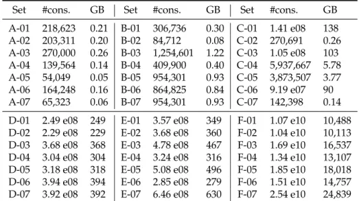
Chapter 2 presents constraints and requirements of the WSRP. It shows math-ematical models formulated in the literature to tackle the WSRP. The mathem-atical formulations are used in the implementation of the HHC instances used throughout this thesis. This chapter also describes information about HHC in-stances and the computational results from applying the MIP solver to those real-world scenarios. Finally, this chapter describes the amount of resources required to solve this problem by the MIP solver. The computational study shows some HHC instances can be solved optimally by the mathematical pro-gramming solver. These results are then set as benchmark results to which the quality of other heuristic solutions can be compared. However, for the other 24 instances, the mathematical programming solver requires computa-tional memory more than 100 GB limits. An estimation shows the largest in-stance may require up to 24 TB of RAM. The result of the study, particularly with the 24 larger instances, reveals challenges to tackle these problem using the mathematical programming solver. This leads to investigations taken in the

(30)

other following chapters.

Chapter 3 describes decomposition methods used in the literature. This chapter also presents an implementation of a decomposition method, the Dantzig-Wolfe decomposition. A computational study using the decomposition on the HHC instances is presented. This clearly shows that HHC instances are difficult as the Dantzig-Wolfe decomposition cannot bring enough of an improvement to the solution. Alternatively, the chapter also reviews the use of heuristic de-composition methods. These heuristic dede-composition methods can solve the other combinatorial problems, i.e. vehicle routing problem, which motivates the development of the heuristic decomposition method to tackle HHC.

Chapter 4 proposes a heuristic decomposition, geographical decomposition with conflict avoidance approach (GDCA). This method decomposes a problem heuristically. It splits a problem into sub-problems by geographical regions. To avoid conflict, this approach requires a sub-problem solving order. Such a solving order could give a distinct solution. Therefore, we executed two exper-iments: applying all possible solving orders to small instances, and applying a defined solving order rules to every instance. We also present an experiment to find a sub-problem order which can produce an acceptable solution.

An extension of GDCA is also given in this chapter. The extension finds a neighbour workforce, which lives nearby the geographical region but is not available on the region, to act as reinforcements. Assignments made to neigh-bour workforce will result in reducing the number of unassigned visits and adding soft constraint violations. Note that the cost of an unassigned visit is less than the soft constraint violation cost. The computational results show a reduction on computational requirements in which the GDCA finds a feasible solution for every HHC instance in a time limit. The solution quality is in an acceptable range, 30% relative gap to the optimal solution on average. How-ever, there is room for improvements in both computational time and solution

(31)

quality.

Chapter 5 proposes an improved heuristic decomposition which does not require a solving order. We propose two variants of this heuristic decompos-ition approach: geographical decomposdecompos-ition with conflict repair (GDCR) and repeated decomposition and conflict repair (RDCR). This heuristic approach does not avoid conflicting assignments. Therefore, a conflicting assignments repair is introduced here to fix the conflicting assignments. However, the repair process might cancel some assignments made by decomposition. Those unas-signed are tackled in two different variants: heuristic assignment in GDCA or using iterative process in RDCR. This chapter also tests an effect of applying different decomposition rules. Finally, it proposes a decomposition rule that is relatively faster and better than the conflict avoidance method.

Chapter 6 applies one of the method proposed in Chapter 5, the repeated decomposition and conflict repair (RDCR), to the WSRP with time-dependent activities constraints. We cannot apply the decomposition method directly be-cause the conflicting assignment repair step may rearrange assignment times which potentially violate time-dependent activities constraints. Therefore, a modification to time-dependent activities constraints is applied. The first modi-fication is made to the process of generating decomposition sub-problem, in which time-dependent activities are grouped in the same sub-problem. The solution to a sub-problem satisfies the time-dependent activities constraints. The time-dependent assignments are then fixed to preserve the time-dependent activities constraint satisfaction even if these assignments has time conflicts with the other assignments, which is then resolved by the conflicting assign-ments repair. A computational study compares the RDCR solutions with a greedy heuristic algorithm proposed in [36]. The results show the RDCR provides a slightly higher number of better solutions.

(32)

trans-forms a full model proposed in Chapter 2 into a smaller one. Thus, a compact model to solve HHC instances is proposed, in which the number of constraints is much smaller than the full model. This compact model requires a differ-ent data format in response to the differdiffer-ent model constraints. Therefore, we also present a reformulation process to the data instance. The full data is com-pressed into three matrices which present 1) time conflicting between visits, 2) compatibility of workforce to take visits, and 3) the total assignment costs. The compact model is then solved to optimality by a mathematical programming solver. The solution to the small model is then transformed back to the solution format supported by the full model so that comparison between algorithms can be made.

Chapter 8 sums up the contribution of this thesis and presents research dir-ections on this topic for future research.

1.4 List of Publications

1. Wasakorn Laesanklang and Dario Landa-Silva. Mixed-integer

program-ming for the workforce scheduling and routing problem.InInternational

Conference on Applied Mathematical Optimization and Modelling (APMOD

2014), pp. 34, 2014, Abstract Only.

2. Wasakorn Laesanklang, Dario Landa-Silva and J. Arturo Castillo-Salazar.

Mixed Integer Programming with Decomposition to Solve a Workforce

Scheduling and Routing Problem. In Proceedings of the 4th International

Conference on Operations Research and Enterprise Systems (ICORES 2015), pp.

283–293, Scitepress, Lisbon, Portugal, January 2015, Best Student Paper Award.

(33)

and Dario Landa-Silva.Extended Decomposition for Mixed Integer

Pro-gramming to Solve a Workforce Scheduling and Routing Problem. In

Operations Research and Enterprise Systems, Series Communications in

Com-puter and Information Science, Vol. 577, pp. 191–211, Springer, 2015. 4. Wasakorn Laesanklang, Dario Landa-Silva and J. Arturo Castillo-Salazar.

Mixed Integer Programming with Decomposition for Workforce

Schedul-ing and RoutSchedul-ing With Time-dependent Activities Constraints. In

Pro-ceedings of the 5th International Conference on Operations Research and

Enter-prise Systems (ICORES 2016), pp. 283–293, Scitepress, Rome, Italy,

Febru-ary 2016.

5. Wasakorn Laesanklang and Dario Landa-Silva.Decomposition Techniques with Mixed Integer Programming and Heuristics to Solve Home

Health-care Planning Problems.Annals of Operations Research,

doi:10.1007/s10479-016-2352-8, 2016.

6. Wasakorn Laesanklang, Dario Landa-Silva and J. Arturo Castillo-Salazar.

An Investigation of Heuristic Decomposition to Tackle Workforce

Schedul-ing and RoutSchedul-ing With Time-dependent Activities Constraints.

submit-ted, to be appear in Operations Research and Enterprise Systems, Series Com-munications in Computer and Information Science.

(34)

Chapter 2 Mixed Integer Programming for a

Workforce Scheduling and Routing

Problem

This chapter focuses on the problem to be solved in this thesis. The main prob-lem is a home healthcare probprob-lem (HHC) which is a variant of a workforce scheduling and routing problem (WSRP). The HHC problem has almost the same component as the WSRP, except that it has fixed time windows and does not have time-dependent activities constraints. HHC instances are described in Section 2.5. Methods proposed in this thesis all aim to to solve the HHC problem, except methods in Chapter 6 which aim to solve the WSRP with time-dependent activities constraints (more details inside the chapter).

This chapter provides background knowledge for the WSRP, a review of the literature for WSRP mathematical models, the HHC problem and our imple-mented MIP model, the HHC instances to be used throughout this thesis, and its solutions producing by a MIP solver.

The MIP model in this chapter has been presented in the following papers: • Wasakorn Laesanklang, Rodrigo Lankaites Pinheiro, Haneen Algethami

(35)

and Dario Landa-Silva.Extended Decomposition for Mixed Integer

Pro-gramming to Solve a Workforce Scheduling and Routing Problem. In

Operations Research and Enterprise Systems, Series Communications in

Com-puter and Information Science, Vol. 577, pp. 191–211, Springer, 2015.

• Wasakorn Laesanklang and Dario Landa-Silva. Decomposition Techniques with Mixed Integer Programming and Heuristics to Solve Home

Health-care Planning Problems.Annals of Operations Research, online-first, 2016.

2.1 Workforce Scheduling and Routing Problem

The Workforce Scheduling and Routing Problem (WSRP) is to address the schedul-ing of mobile personnel visitschedul-ing different locations [35]. Examples of WSRP Scenarios include home healthcare, home care, scheduling technicians, secur-ity personnel routing and rostering, and manpower allocation. An assumption when defining a problem to be WSRP is that the workforce should spend more time doing work than travelling. Therefore, the focus of the business is to de-liver the right services to its customers.

Table 2.1 presents WSRP characteristics and their definition which are found in the literature. The first column shows types of characteristic and the second column presents a definition of each characteristic. There are 7 characteristics which are summarised by Castillo-Salazar et al. [35]: time windows, skills and qualifications, service time, start and end locations, connected activities, and teaming.

1. Time Windows

A time window indicates the time by which the activity must start [118]. The values are commonly presented as the earliest starting time and the latest starting time for each visit. A visit to be made must start within the

(36)

Table 2.1:WSRP constraints in the literature

Constraint Definition

Time Windows A time interval for starting a visit. Workforce can start the work as soon as they reach the working location in between the inter-val. Time windows can be flexible or tight depending on problem requirements. An exact time window is also possible, i.e. a visit must start at the appointment time.

Skills and Qualifications Only qualified workforce can work on a visit which requires primary skills. Generally, an organisation has diversity of skilled workforce. Hence, assigning under-skilled workforce is prohib-ited. Some cases also require the minimisation of assigning over-qualified workforce as they should be preserved for the high skill requirement only.

Service Time A duration of a working visit. In reality, the duration is very dependent on an individual worker. In practice, the service time is assumed to be of a fixed duration.

Start and End Locations Workforce may (leave from/return to) a single starting location (office), or many locations (i.e. from their home). Starting loca-tion and ending localoca-tion may be defined as different places. Connected Activities Two or more visits may depend on each other. It includes

sequen-tial dependency (a visit must be performed before the other), syn-chronisation (visits start at the same time), overlap (the second visit starts while another visit is in progress) and dependency with time differences (sequenced visits with a break interval and/or expired time before starting the next visit).

Teaming Visits require a group or team to participate. Problem of having fixed teams, because they are not changed for the whole plan. This case may define a team as a single worker. The other cases show team may be changed during the time horizon. For ex-ample, a worker may join a team during his morning visit and join the other team in the afternoon.

Clusterisation Visits are grouped in clusters or zones. It may apply to prevent assigning a worker long distances to travel. It also can be used to reduce the size of the problem by tackling sub-problems instead of the whole problem.

(37)

time interval. The time window interval shows a flexibility of the visit. A visit with time-wised priority usually has a narrower time window in-terval, e.g. a visit for patient to have medicine should have 10 minutes of time window interval. In some cases, the time window interval has length 0, i.e. the earliest start time is equal to the latest start time, which is called anexact time window[61]. This exact time window case appears in the home healthcare scenarios which are used throughout this thesis.

2. Skills and Qualifications

Skills and qualifications are values to narrow the candidate workers down. In this case, a visit must be made by workers who have the required skills. A problem might define workers with no differences in skills, called uni-skill worker [15, 67, 75, 127]. The uni-uni-skill problem usually is a simpli-fied case which only arranges the number of workers for each working shift. However, problems related to the real-world usually have multiple skills. The hierarchical skill is when higher ranked skills can substitute lower ranked skills, and the reverse is not valid [19, 114, 122]. The worker with higher ranked skills is known as a specialist and the worker with lower ranked skills is defined as a generalist. Assigning an over qualified worker might result in penalty costs in the proposed solution. The multi-skill case is when two different multi-skills cannot be replaced by each other. A job requirement may state a combination of skills [64, 70, 81]. How-ever, the real world problem usually has a combination of multiple and hierarchical skills [38]. In summary, workforce scheduling is to allocate qualified workers for jobs that have certain skills demands.

3. Service Time

A service time is a duration that workers must spend when they make a visit. Generally, the service time is tackled as a fixed value for each visit.

(38)

However, the duration might be defined based on worker’s skills, e.g. a worker with higher ranked skills should take less time on a visit com-pared to a worker who has lower ranked skills. This latter case is rarely found in the literature because it adds difficulties of the problem and some cases may require workers to attend a visit for the whole duration.

4. Start and End Locations

Workers can start and end their journey at any location depending on the type of the problem. A start and end location can be a single point, called a single depot problem [37, 40, 79, 118]. The problem can be extended to a multiple depots problem when a worker starts and finishes their journey at the same location but different workers may have different depots [48, 53, 88]. An example is the case that workers leave their home for work and finally finish the day by returning to their home. The other case is the combination of single depot and multiple depot, i.e. workers must start their work from the central depot but they can go straight to their home after they complete the last visit.

5. Connected Activities

This characteristic explains a visit that may depend on another visit. Con-nected activities may be defined in a time-based restriction, known as

time-dependent activities[107]. There are five types of time-dependent

activ-ities: synchronise, overlap, minimum difference, maximum difference, and min-max difference. The time-dependent activities will be further ex-plained intime-dependent activities constraints which appears later in this chapter.

6. Teaming

Some visits may require a team due to the nature of the work [82]. Team members may remain unchanged throughout the planning horizon which

(39)

a whole team is can be considered as a single person. Although, the gen-eralised problem should consider temporally teams, i.e. a team is formed just for a required visit and its members can travel to different locations and continue on to other visits. This case might be considered as a group of synchronised visits which requires multiple visits to be made at the same time.

7. Clusterisation

Visits might be grouped when they are located in the same regions e.g. the same building, the same street or the same county. A reason behind clusterisation is that workers usually not prefer to work too far away from their home. As a result, workers may choose a set of regions they prefer. Additionally, clusterisation might be used to reduce the number of visits by considering a group as a single visit location which then decreases the problem difficulty.

WSRP scenarios may have their specific features depending on their real-world application. We choose home healthcare (HHC) scenarios as an example, with its requirements given by our industrial partner. We remind the reader that the HHC problem is to allocate care workers to make visits at to homes of the patients. In practice, patients or customers usually order regular visits, e.g. a visit every Monday at 10 AM. We note that this problem is an exact time window problem.

Each visit requests workers with multiple skills which can be expressed into two sets: minimum skill requirements and additional skill requirements. Work-ers who will make the visit must at least have the minimum skill requirements and workers who have the additional skills are preferable. A patient may re-quest a team to make visits. For this problem, temporally team approach is applied, i.e. a nurse and a doctor are met at patient home, so the team can be

(40)

split thereafter. A visit requires a fixed service time, i.e. workers must stay with the patient for the whole duration.

The HHC is a multiple depots problem because care workers prefer to leave for work from their home. The problem also assumes that workers return to their home after they finish their tour. The problem also clusters visits into geo-graphical regions. Workers also have their responsibility regions and preferred regions. The scheduler should assign visits located in worker’s responsibility regions. However, the problem does not take this as a strict condition because realistically a worker can make visits outside their responsibility regions. Work-ers also have their working times so visits assigned to workWork-ers should lie within their working period. However, workers might be requested to make visits out-side their working times. We note that some visits may be left unassigned due to lack of skilled workers. The value of unassigned visits are very important to our industrial partner to estimate their limitation and which possibly a future improvement to their services.

A solution to the WSRP is evaluated by multiple criteria, for example: trav-elling distances, travtrav-elling times, operational costs, workforce efficiency, work-force/client preferences and the number of unassigned visits. These multiple aspects can be tackled as a multi-objective problem [9, 18]. The multi-objective approach finds multiple solutions and leave decision makers to choose which solution they will use [24]. These solutions must not be completely dominated by the other solutions, i.e. all quality measure values of the completely domin-ated solution are lower than a dominating solution. This approach requires a large computational time to provide a set of non-dominated solutions. Altern-atively, a single objective approach can be used if the decision maker has a rule for decision making. The rule is then converted to a mathematical function, called weighted-sum, which is a summation of the weighted quality measure value, where the weights are provided by decision maker.

(41)

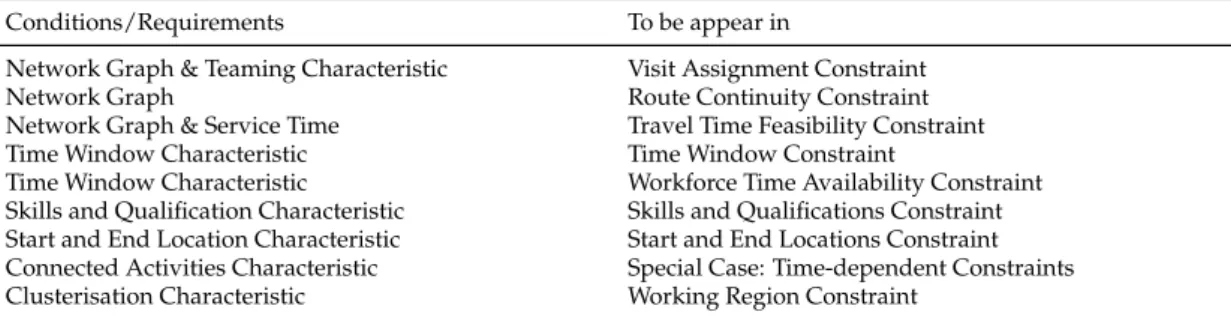
Table 2.2:Relation between WSRP conditions/requirements and WSRP con-straints to be implemented in MIP model

Conditions/Requirements To be appear in

Network Graph & Teaming Characteristic Visit Assignment Constraint Network Graph Route Continuity Constraint Network Graph & Service Time Travel Time Feasibility Constraint Time Window Characteristic Time Window Constraint

Time Window Characteristic Workforce Time Availability Constraint Skills and Qualification Characteristic Skills and Qualifications Constraint Start and End Location Characteristic Start and End Locations Constraint Connected Activities Characteristic Special Case: Time-dependent Constraints Clusterisation Characteristic Working Region Constraint

2.2 Literature Review

The problem characteristics from the previous section leads us to the WSRP constraints and their implementation. Before explaining the details of each con-straint, this section starts with explanation of general concept of mathematical models.

MIP models defining the WSRP are usually formulated as a flow model [26]. Generally, a directed graph G = (V,E) represents the network flows, where

V is a set of nodes to represent visits and start-end locations and E is a set of edges between nodes which each edge presents a travel route between two visits. The problem is to find paths along edges that set off from starting nodes, then pass the visiting nodes and reach the ending nodes, while maximising the number of nodes to be visited. The maximum number of paths is equal to the number of workers. The network model has been applied to other problem such as scheduling problems, and routing problems. In addition, constraints of the scheduling problem and the routing problem can be adopted for the WSRP because they share the graph structure.

Problem characteristics and the network structure are defined as constraints in MIP models as shown in Table 2.2. Table 2.2 presents two columns to re-late the problem characteristics and the network structure of the problem with the constraints implemented in the MIP model. In mathematical programming problem, constraints are treated as boundaries of search space in which feasible

(42)

solutions are located inside the border (including the border line), known as feasible regions. These constraints are generally explained in mathematical for-mulations. The objective function can be used to evaluate the solution quality. Both objective function and constraints are very important in a mathematical programming problem [23].

There are common constraints where most of the MIP models in the literat-ure are implemented and problem specific constraints which are defined to spe-cific problem requirements. We argue that an integration of constraints presen-ted in the literature might cover the most of existing real-world requirements. In this thesis, we describe details of five selected mathematical models from the literature: Bredstrom and Ronnqvist [26], Rasmussen et al. [107], Dohn et al. [55], Trautsamwieser and Hirsch [121], and Barrera et al. [13].

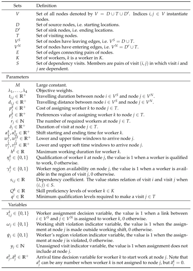
Table 2.3 lists the notation of sets, parameters, and variables for explaining mathematical models in the literature, and the proposed mixed integer pro-gramming model presented later in this chapter. This notation will be used throughout this thesis. The domain of notation presented in this table is presen-ted based on the proposed mixed integer programming model to solve HHC problem which is explained in Section 2.4. Here, we use the same notation in every model to present the notations with the same meaning. Although, there might be differences in their domains, i.e. yjis a binary variable in [107], butyj in our implemented model is an integer variable. This is because models in the literature have different implementation concepts.

(43)

Table 2.3:Notation used in MIP model for WSRP

Sets Definition

V Set of all nodes denoted byV = D∪T∪D0. Indices i,j ∈ V instantiate nodes.

D Set of source nodes, i.e. starting locations. D0 Set of sink nodes, i.e. ending locations.

T Set of visiting nodes.

VS Set of nodes have leaving edges, i.e.VS =D∪T. VN Set of nodes have entering edges, i.e.VN=D0∪T.

E Set of edges connecting pairs of nodes. K Set of workers,kis a worker inK.

S Set of dependency visits. Members are pairs of visit(i,j)in which visitiand jare dependent.

Parameters

M Large constant.

λ1, . . . ,λ4 Objective weights.

ti,j ∈R+ Travelling duration between nodei∈VSand nodej∈VN.

di,j ∈R+ Travelling distance between nodei∈VSand nodej∈VN.

pk_j ∈R+ _{Cost of assigning worker}_k_{to node}_j_∈_T.

ρk_j ∈R+ Preferences value of assigning workerkto nodej∈T.

rj ∈N The number of required workers at nodej∈T.

δj∈R+ Duration of visit at nodej∈T.

αk_L,αk_U ∈R+ Shift starting and ending time for workerk.

wL_j,wU_j ∈R+ _{Lower and upper time windows to arrive node}_j.

vL

j,vUj ∈R+ Lower and upper soft time windows to arrive nodej.

hk _∈_R _{Maximum working duration for worker}_k.

ηk_j ∈ {0, 1} Qualification of workerkat nodej, the value is 1 when a worker is qualified

to work, 0 otherwise.

γk_j ∈ {0, 1} Worker region availability on nodej, the value is 1 when a worker is

avail-able in the region of visitj, 0 otherwise.

si,j∈R Dependency coefficient. The value states relation of visitiand visitjwhen

(i,j)∈S.

Qk _∈_R _{Skill proficiency levels of worker}_k_∈_K

qj∈R Minimum qualification levels required to make a visitj∈T Variables

xk_i_,_j∈ {0, 1} Worker assignment decision variable, the value is 1 when a link between i∈VSandj∈VNis assigned to workerk, 0 otherwise.

ωj ∈ {0, 1} Working shift violation indicator variable, the value is 1 when the

assign-ment at nodejis made outside working shift, 0 otherwise.

ψj∈ {0, 1} Worker’s region violation indicator variable, the value is 1 when the

assign-ment at nodejis violated, 0 otherwise.

yj ∈N Unassigned visit indicator variable, the value is 1 when assignment does not

include at nodej.

ak_j, ˜ak_j ∈R+ _{Arrival time decision variable for worker}_k_{to start work at node}_{j. Note that}

(44)

2.3 Constraints for Workforce Scheduling and

Rout-ing Problem in the Literature

This section analyses constraints implemented on the five selected mathemat-ical models listed above. For simplicity, we use the following short-hand nota-tion to refer to each of the five works:

• ODS-HHC: Optimisation of Daily Scheduling for Home Health Care Ser-vices [121],

• NB-TCS: A Network-based Approach to the Multi-activity Combined Time-tabling and Crew Scheduling Problem: Workforce Scheduling for Public Health Policy Implementation [13],

• VRS-TPS: Combined Vehicle Routing and Scheduling with Temporal Pre-cedence and Synchronization Constraints [26],

• MAP-TTC: The Manpower Allocation Problem with Time windows and Job-teaming Constraints [55], and

• HCS-PCD: The Home Care Crew Scheduling Problem: Preference-based visit clustering and temporal dependencies [107].

Generally, each paper defines its own set of notations to explain its mathem-atical model. However, to make comparisons between models, the notations presented in this thesis are normalised to the same set presented in Table 2.3.

Each constraint is presented individually to compare the five implementa-tion approaches.

2.3.1 Visit Assignment Constraints

This constraint indicates that visits require a worker. It is the backbone of many problems as it pairs workers to attending visits. Table 2.4 compares the visit

(45)

Table 2.4:Visit assignment constraint comparison between five different math-ematical models.

Visit assignment constraint

ODS-HHC All visits need a worker to visit. No unassigned visit allowed.

Hard constraint:

∑

i∈VS_k

∑

∈K

x_ik_,_j =1∀j∈T

NB-TCS All demands need to be filled. Only qualified workforce

indic-ated by a binary parameter can be selected. Assigned visit must

be balanced amongst workforce. bis a variable for maximum

workload differences between workers.

Hard constraint:

∑

k∈Ki∈

∑

VS ηk_jxk_i_,_j =rj ∀j∈T, η_jk, rjare binary Balance assignment:

∑

i,j∈V δjxk_i_,1_j −

∑

i,j∈V δjxk_i_,2_j ≤ b ∀k1,k2 ∈ K : k1 6= k2

Balance objective: Minimiseb

VRS-TPS All visits need a visit. No unassigned visit allowed. bis a

vari-able for maximum workload differences between workers.

Hard constraint:

∑

k∈Ki∈

∑

VS x_ik_,_j =1∀j∈T Balance assignment:

∑

i,j∈V δjxki,1j−

∑

i,j∈V δjxik,2j ≤b∀k1,k2 ∈K:k16=k2

Balance objective: Minimiseb

MAP-TTC Visiting must not exceed demand. Note that objective is to

max-imise the number of assignments made.

Hard constraint:

∑

k∈Ki∈

∑

VS

x_ik_,_j ≤rj∀j∈ T

Obj. function: max

∑

k∈Ki∈

∑

VS_j_∈

∑

_VN

x_ik_,_j

HCS-PCD Soft constraint where unassigned visits are charged in objective

function.

Soft constraint:

∑

i∈VS_k

∑

∈K

x_ik_,_j+yj =1∀j∈ T

Obj. function: Min

∑

j∈T yj

assignment constraint for the five mathematical models.

This constraint can be implemented by simply stating that every visit needs exactly one worker as in models ODS-HHC and VRS-TPS. These two models consider visit assignment as a hard condition where all visits must be made. On

(46)

the other hand, a soft condition implementation of this constraint can be done as presented in model HCS-PCD. As such, visits are allowed to be unassigned but need to be minimised. Models NB-TCS and MAP-TTC tackle this constraint by stating visiting demand explicitly such as that visit jmust havebj workers to visit.

The assignment may also require balancing the workload amongst work-ers as in models NB-TCS and VRS-TPS. These models introduced additional decision variablebwhich is the maximum number of assignments per worker. The value needs to be minimised which ideally gives a solution with a balanced workload.

The visit assignment constraint has been implemented in the same direc-tion, i.e. entering edges of a visiting node must be selected. The number of entering edges to be selected is equal to the number of visiting demand. The hard condition interpretation of the visiting constraint is suitable for problems which have been shown that all visits can be logically made, i.e. the number of skilled workers is sufficient to all visits. The interpretation which suitable for the real-world problems considered here is the soft condition interpretation where unassigned visits are allowed. A solution with unassigned visits could reflect causes of problems in operations such as overbooking, worker short-ages, or skilled worker shortages. Therefore, the constraint to be implemented for a general WSRP is required to support the multiple visiting demand prob-lem which is impprob-lemented as a soft condition (see Section 2.4.1). This results in mixing constraints of two models NB-TCS and HCS-PCD.

2.3.2 Route Continuity Constraints

This is commonly defined as flow conservation constraint and it states that the number of entering flows must be equal to the number of leaving flows. In the WSRP context, the number of flows refers to the number of visiting

(47)

work-Table 2.5:Route continuity constraint implemented on five mathematical models.

Route continuity constraint.

ODS-HHC _{Flow conservation constraint. At a visit, the number of}

enter-ing workers must be equal to the number of leaventer-ing workers.

Hard constraint:

∑

i∈VS xk_i_,_h=

∑

j∈VN x_hk_,_j ∀h∈T,∀k∈K NB-TCS VRS-TPS MAP-TTC HCS-PCD

ers. Hence, the route continuity constraint states that the number of workers arriving to a visit must be the same as the number of workers leaving the visit. Table 2.5 shows the mathematical formulation used in all the five mathematical models to implement this constraint. The same constraint is used in our WSRP model (see Section 2.4.2).

The route continuity constraint presented by all the five models is a typ-ical flow conservation constraint. The mathemattyp-ical formulation shown in the table is in the compact form to describe this constraint which has been shown to be efficient as we can find it implemented in the five models. However, this constraint alone may not enforce a working path, for example, a cycle xk_i_,_i = 1 is feasible by this constraint where the cycle is not satisfied the WSRP because the cycle does not make progress from starting location and terminate at the ending location. Therefore, cycle cases are eliminated from the WSRP solution by travel time feasibility constraints (see 2.3.4). In addition, a complete path requires a starting location and an ending location where those locations are defined in constraint start and end location (see 2.3.3). However, the route con-tinuity constraint is the only formulation to define links between visits which is a backbone of the solution.

2.3.3 Start and End Locations Constraints

Start and end locations are general requirements for flow models. They are special nodes which only have one direction to connect to other nodes. Strictly

(48)

speaking, the start location has only leaving edges and the end location has only entering edges. They are places for distributing workers and collecting them when they finish their journey. Table 2.6 shows the mathematical formulation of start and end locations on the five selected models. There are implement-ations in both single central location and multiple locimplement-ations cases. The single central location has only one centre point to distribute all workers. The mul-tiple locations case is when workers can start their journey from their chosen place, i.e. their home.

Most models implement this constraint by forcing all workers to leave from starting locations and return back to the ending location. Only ODS-HHC does not have this approach, so that using all workers is not required. These condi-tions were subject to requirements of each model.

A single central location problem, as shown in models VRS-TPS, MAP-TTC and ODS-HHC, assumes there is only one location for the start and end of a worker’s route. It applies to general cases where workers need to visit their office before being deployed for work. We denote 0 is an index to represent the central location in models ODS-HHC and MAP-TCC. The constraint means a worker must leave the start location only/at most once. The same requirement applies to end location. Note that the model VRS-TPS shows the formulation for multiple depots but the problem instances tackled in this work only con-sidered a single location.

The NB-TCS model also defines a single location problem. However, the assignment constraints include the condition to control assignments from start to finish. As such, there is no explicit implementation of this condition.

The HCS-PCD model has multiple start and end locations. The case repres-ents a problem with multiple offices or if workers are able to start their journey from their home. The implemented constraint only applies to worker k and their selected start location and edges connecting between the workerkand the

Heuristic decomposition and mathematical programming for workforce scheduling and routing problems

Laesanklang, Wasakorn (2017) Heuristic decomposition

and mathematical programming for workforce

scheduling and routing problems. PhD thesis, University

of Nottingham.

Heuristic Decomposition and

Mathematical Programming for

Workforce Scheduling and

Routing Problems

Wasakorn Laesanklang

Thesis submitted to the University of Nottingham

for the degree of Doctor of Philosophy

Abstract

Contents

List of Figures

List of Tables

Acknowledgements

Chapter 1

Introduction

1.1

Background and Motivation

1.2

Summary of Contributions

1.3

Structure of Thesis

1.4

List of Publications

Chapter 2

Mixed Integer Programming for a

Workforce Scheduling and Routing

Problem

2.1

Workforce Scheduling and Routing Problem

2.2

Literature Review

2.3

Constraints for Workforce Scheduling and

Rout-ing Problem in the Literature

2.3.1

Visit Assignment Constraints

∑

∑

∑

∑

∑

∑

∑

∑

∑

∑

∑

∑

∑

∑

∑

∑

∑

∑

2.3.2

Route Continuity Constraints

∑

∑

2.3.3

Start and End Locations Constraints