A randomized web-cache replacement scheme

(1)

A Randomized Web-Cache Replacement Scheme

Konstantinos Psounis , Balaji Prabhakar

Department of Electrical Engineering

Departments of Electrical Engineering and Computer Science

Stanford University

Stanford, CA 94305

[email protected], [email protected]

Abstract—

The problem of document replacement in web caches has received much attention in recent research, and it has been shown that the eviction rule “replace the least recently used document” performs poorly in web caches. Instead, it has been shown that using a combination of several criteria, such as the recentness and frequency of use, the size, and the cost of fetching a document, leads to a sizeable improvement in hit rate and latency reduc-tion. However, in order to implement these novel schemes, one needs to maintain complicated data structures. We propose randomized algorithms for approximating any existing web-cache replacement scheme and thereby avoid the need for any data structures.

At document-replacement times, the randomized algorithm samples documents from the cache and replaces the least useful document from the sample, where usefulness is determined according to the criteria mentioned above. The next least useful documents are retained for the suc-ceeding iteration. When the next replacement is to be performed, the algo-rithm obtains new samples from the cache, and replaces the least

useful document from the new samples and the previously

re-tained. Using theory and simulations, we analyze the algorithm and find that it matches the performance of existing document replacement schemes for values of and as low as 8 and 2 respectively. Rather surprisingly, we find that retaining a small number of samples from one iteration to the next leads to an exponential improvement in performance as compared to retaining no samples at all.

Keywords— Web caching, document replacement policies, randomized algorithm.

I. INTRODUCTION

HE enormous popularity of the World Wide Web in recent years has caused a tremendous increase in network traffic due to HTTP requests. Since the majority of web documents are static, caching them at various network points provides a natu-ral way of reducing traffic. At the same time, caching reduces download latency and the load on web servers.

A key component of a cache is its replacement policy, which is a decision rule for evicting a page currently in the cache to make room for a new page. The rule that replaces the least cently used (LRU) page from the cache, is the most popular re-placement policy. This is due to a number of reasons: LRU is an optimal online algorithm in the competitve ratio sense1_{, it only}

requires a linked list to be efficiently implemented as opposed to more complicated data structures required for other schemes, and takes advantage of temporal locality in the request sequence

2_.

This research is supported in part by a Stanford Graduate Fellowship, and a Terman Fellowship.

LRU is -competitive and there is no deterministic online algorithm with a competitive ratio smaller than [7].

A sequence of requests is said to exibit temporal locality if the probability to request an object after requests, given that it was just requested, is inversly proportional to .

Suppose that we associate with any replacement scheme a

utility function, which sorts pages according to their suitability for eviction. For example, the utility function for LRU assigns to each page a value which is the time since the page’s last use. The replacement scheme would then replace that page which is most suitable for eviction.

Whereas for processor caches LRU and its variants have worked very well [11], it has recently been found [2] that LRU is not suitable for web caches. This is because some impor-tant differences distinguish a web cache from a processor cache: (i) The size of web documents are not the same, and (ii) the cost of fetching different documents varies significantly. These differences do not occur in a processor cache. Thus, a util-ity function that takes into account not only the popularutil-ity of a web document, but also its size and cost of fetching can be expected to perform significantly better. Recent work pro-poses many new cache replacement schemes that exploit this point (e.g. LRU-Threshold[1], GD-Size[2], GD*[5], LRV[6], SIZE[12], Hybrid[13]).

However, the data structures that are needed for implementing these new utility functions turn out to be complicated. Most of them require a priority queue in order to reduce the time to find

a replacement from to , where is the number

of documents in the cache. Further, these data structures need to beconstantly updated(i.e., even when there is no eviction), although they are solely used for eviction.

This prompts us to consider randomized algorithms which do not need any data structures. For example, the particularly simple Random Replacement (RR) algorithm evicts a document drawn at random from the cache [7]. However, as might be ex-pected, the RR algorithm does not perform very well.

We propose to combine the benefits of both the utility func-tion based schemes and the RR scheme. Thus, consider a scheme which draws documents from the cache and evicts the least useful document in the sample. The “usefulness” of a document is as determined by the utility function. Although this basic scheme performs better than RR for small values of , we find a tremendous improvement in performance by refining it as follows: After replacing the least useful of samples, the identity of the next least useful documents is retained in memory. At the next eviction time, new samples are drawn from the cache and the least useful of these and previously retained is evicted, and the identity of the least useful of the remaining is stored in memory, and so on.

(2)

few randomly drawn samples depends on the quality of the sam-ples. Therefore, by deliberately tilting the distribution of the samples towards the good side, which is precisely what the re-finement achieves, one expects an improvement in performance. Rather surprisingly, we find that the performance improvement can beexponentialfor small values of (e.g. 1, 2 or 3).

The rest of the paper is organized as follows. In Section II we present the randomized algorithm, and in Section III we an-alyze it. In particular, we find that a small value of leads to a big improvement in performance compared to when . On the other hand, we find that choosing too high a value of degrades the performance, since we will have too few fresh samples. Section IV investigates the variation in performance as increases from 0 to . Specifically, we prove that the per-formance of the algorithm is convex in with most the benefit obtained for small values of . In Section V we derive a simple approximate closed form formula for the optimal value of as a function of . Section VI presents trace driven simulations comparing the randomized scheme with various existing deter-ministic schemes. We find that even with small values of and (e.g. 8 and 2 respectively) the randomized scheme performs very competitively. Section VII concludes the paper.

II. A DESCRIPTION OF THEALGORITHM

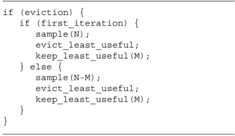
The first time a document is to be evicted, samples are drawn at random from the cache and the least useful of these is evicted. After replacing the least useful document from the sample, the next least useful documents are retained for the next iteration. And when the next replacement is to be performed, the algorithm obtains new samples from the cache, and replaces the least useful document from the

new samples and the previously retained. This procedure is repeated whenever a document needs to be evicted. Figure 1 presents the algorithm in pseudo-code.

if (eviction) { if (first_iteration) { sample(N); evict_least_useful; keep_least_useful(M); } else { sample(N-M); evict_least_useful; keep_least_useful(M); } }

Fig. 1. The randomized algorithm.

An error is said to have occurred if the evicted documentdoes notbelong to the least useful percentile of all the documents in the cache, for some desirable values of . Thus, the goal of the algorithm we consider is to minimize the probability of error. We shall say that a document isuselessif it belongs to the least useful percentile3_.

Note that samples that are good eviction candidates will be called “useless” samples since they are useless for the cache.

It is interesting to conduct a quick analysis of the algorithm described above in the case where so as to have a bench-mark for comparison. Accordingly, suppose that all the docu-ments are divided into bins according to usefulness and documents are sampled uniformly and independently from the cache. Then the probability of error equals ,4

which approximately equals . By increasing this

probability can be made to approach 0 exponentially fast. (For

example, when and , the probability of error is

approximately 0.08. By increasing to 60, the probability of error can be made as low as 0.0067.)

But it is possible to do much better without doubling ! That

is, even with , by choosing , the probability

of error can be brought down to . In the next few

sections we obtain models to further understand the effect of on performance.

We end this section with the following remark. Whereas it is possible for a document whose id is retained in memory to be accessed between iterations, making it a “recently used doc-ument”, we find that in practice the odds of this happening are negligibly small5_{. Hence, in all our analysis, we shall assume}

that documents which are retained in memory are not accessed between iterations.

III. THEMODEL ANDPRELIMINARYANALYSIS In this section we derive and solve a model that describes the behavior of the algorithm precisely. We are interested in com-puting the probability of error, which is the probability that none of the documents in the sample is useless for the cache, for

any given and and for all .

We proceed by introducing some helpful notation. Of the samples retained at the end of the iteration, let

( ) be the number of useless documents. At the

beginning of the iteration, the algorithm chooses

fresh samples. Let , be the number of

useless documents coming from the fresh samples. In the iteration, the algorithm replaces one document out of

the total available (so long as )

and retains documents for the next iteration. Note that it is possible for the algorithm to discard some useless documents because of the memory limit of that we have imposed.

Define to be precisely the

number of useless documents in the sample just prior to the document replacement, that the algorithm would ever replace at eviction times. If , then the algorithm commits an error at the eviction. It is easy to see that is a Markov chain and satisfies the recursion

and that is binomially distributed with parameters

and . For a fixed and , let ,

, denote the probability that useless documents for the cache, and thus good eviction candidates, are acquired during a sampling. When it is clear from the context we will Although the algorithm samples without replacement, the values of are so small compared to the overall size of the cache that almost exactly equals the probability of error.

(3)

X Xm−1 _X_X_m_m AAmm

1

(Xm−1>0)

1

(Xm>0) (m)th (m−1)th (m+1)th

Fig. 2. Sequence of events per iteration. Note that eviction takes place prior to resampling.

abbreviate to . Figure 2 is a schematic of the above Markov chain.

Let denote the transition matrix of the chain for a given value of . The form of the matrix depends on whether is smaller or larger than . Since we are interested in

small values of , we shall suppose that 6_{. It is}

immediate that is irreducible and has the general form

..

. ... ...

As may be inferred from the transition matrix, the Markov chain models a system with one deterministic server, binomial arrivals, and a finite queue size equal to (the system’s overall size is ). An interesting feature of the system is that as

increases, the average arrival rate, ,

decreases linearly and the maximum queue size increases lin-early.

Let denote the stationary distribution of

the chain . Clearly is the probability of error as defined

above. Let be an matrix, with

for all . Let be a matrix

with for all . Since is irreducible, is

invertible [8] and

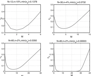
(1) Figure 3 shows a collection of plots of versus for dif-ferent values of and . The minimum value of is written on top of each figure. We note that given and there are values of for which the error probability is very small compared to its value at . We also observe that there is no need for to be a lot bigger than the number of bins for the probability of error to be as close to zero as desired, since

even for the minimum probability of error is

extremely small. Finally, we notice that for small values of there is a huge reduction in the error probability and that the minimum is achieved for a small . As increases further the performance deteriorates linearly.

The exponential improvement for small can be intuitively explained as follows. For concreteness, suppose that

Figure 3 suggests that the at which the probability of error is minimized is less than . 0 2 4 6 0.1 0.2 0.3 0.4 0.5 M π0 N=12,n=10%,min(π₀)=0.1378 0 5 10 15 0 0.1 0.2 0.3 0.4 0.5 M π0 N=30,n=4%,min(π₀)=0.0732 0 10 20 30 0 0.1 0.2 0.3 0.4 0.5 M π0 N=60,n=2%,min(π₀)=0.0350 0 10 20 30 40 0 0.05 0.1 0.15 0.2 0.25 M π0 N=80,n=2%,min(π₀)=0.00003

Fig. 3. Probability of error ( =probability not a useless document for the cache is replaced) versus number of documents retained ( ).

and that the Markov chain has been running from time onwards (hence it is in equilibrium at any time ). The

relationship

imme-diately gives that

. Supposing that ,

and . Therefore

. Compare this number with the case

, where , and the

claimed exponential improvement is apparent.

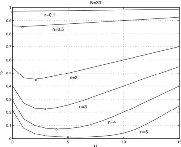
IV. A CLOSERLOOK AT THEPERFORMANCECURVES From Figure 3 it is evident that for the specific values of and used in the plots, as increases from small to large val-ues, the error probability decreases exponentially, flattens out, and then increases linearly. In Figure 4, we plot the error prob-ability for and various small values of , to investigate the behavior of when the value of the sample deteriorates. We observe that in all these curves the error probability is a convex function of , almost always possessing the features mentioned above.

It is therefore interesting to investigate if this convexity holds for any value of and . Before launching into proofs, we briefly give an insight into why the error probability is convex

in .

Fix the values of and and let and be two

instan-tiations of the scheme proposed, with memory sizes of and respectively. Let (respectively, ) be the average arrival rate of useless documents from resampling in system

(respectively, system ). Since

, system gets more useless docu-ments from resampling than system on the average. However, the queue size of system , which equals , is smaller than that of system ’s by one place. Hence there will be times at which system will be full and drop samples, while system will be able to accommodate an extra sample. When increases

(4)

0 5 10 15 0 0.1 0.2 0.3 0.4 0.5 0.6 0.7 0.8 0.9 1 M π0 N=30 n=0.1 n=0.5 n=2 n=3 n=5 n=4 o o o o o o | |

Fig. 4. Convexity of as a function of .

from 0 to 1, the positive effect of an increase in the queue size offsets the negative effect of a decrease in the arrival rate. As increases further, it is less likely for overflows to occur and the dominating phenomenon is the decrease in arrival rate. This trade-off between high arrival rate and high queue size causes to be a convex function of , and thus there is an optimal value of at which is minimized.

To establish convexity directly, it would help greatly if could have been expressed as a function of the elements of

in closed form. Unfortunately, this is not the case and we must use an indirect method, which seems interesting in its own right. Our method consists of relating to the quantity , which is the number of overflows in the time interval from a buffer of size with average arrival rate

. Let

Theorem 1: The probability of error is convex in .

Sketch of proof: Let be the number of arrivals in . Then the probability the system is full as observed by arrivals, or equivalent the probability of drops, equals

Lemma 3 below implies that is convex in .

Proceeding, equating effective arrival and departure rates we obtain

or (2)

Since is linear in , and is

convex in , Equation (2) implies is

convex in .

To complete the proof it remains to show that is con-vex in . The proof of the convexity of is carried out

(M−1) (M) (M+1)

Lemma 1 Lemma 2 Lemma 3

λλ(M−1)λλ(M)λλ(M+1) λλ(M−1)λλ(M)λλ(M+1) λλ(M)

(M) (M) (M) (M−1) (M) (M+1)

Fig. 5. The cases relevant for Lemma 1, Lemma 2, and Lemma 3 respectively.

in Lemmas 1, 2, and 3 below. In the following we

abbrevi-ate to when the arrival process does

not depend on , and to when the buffer size is

constant, regardless of the value of . Lemma 1 shows that

is convex in for all . Lemma 2 shows the

convexity of . Finally, Lemma 3 shows

the convexity of . Figure 5

schematically describes the cases that each lemma deals with. Due to limitations of space, we only give a sketch of the some-what combinatorially involved proofs of these results. The full proofs can be found in [10].

Lemma 1: is a convex function of , for each .

Sketch of proof:To prove convexity it suffices to show that the second order derivative of the number of drops is non-negative; i.e., that

. This can be done by comparing the number of drops

, , and from systems with

buffer sizes , , and respectively, under identical

arrival processes, as shown in figure 5. Essentially, the compar-ison entails considering the situations for buffer occupancies in the three systems that lead to drops.

Let .

Lemma 2: is a convex function of when .

Sketch of proof: We need to show

by considering three sys-tems with same buffer sizes and binomially distributed arrival

processes with average rates , and ,

as shown in figure 5. Thus, there will be common arrivals and exclusive arrivals as categorized below:

(a) An arrival occurs at all three systems.

(b) An arrival occurs only at the system with buffer size . (c) An arrival occurs at the two systems with buffer sizes and and there is no arrival at the system with buffer size

.

Due to the arrival rates being as in the hypothesis of the lemma, category (b) and (c) arrivals are identically distributed. Us-ing this and combinatorial arguments one can then show that

is convex.

Lemma 3: is a convex function of when .

(5)

TABLE I

OPTIMUM VALUES OF AND FOR VARIOUS AND .

=10 =20 =10 =20 8 0.3643 0.0593 1 2 10 0.2450 0.0110 1 3 12 0.1378 0.0011 2 4 =5 =10 =5 =10 20 0.1946 0.0013 2 5 =4 =8 =4 =8 30 0.0732 4 9 =3 =6 =9 =3 =6 =9 40 0.0558 5 12 16 =2 =4 =6 =2 =4 =6 50 0.1354 4 13 18 60 0.0350 - 7 19 -70 0.0025 - - 11 - -80 - - 16 -

-Sketch of proof: We consider three systems of buffer sizes , and , whose arrival processes are Binomially

distributed with rates , and , as shown

in figure 5. This is a combination of Lemma 1 and 2. V. ON THEOPTIMALVALUE OF

The objective of this section is to derive an approximate closed form expression for the optimal value of for a given

and .

Let be the optimal value of . As

remarked earlier, even though the form of the transition matrix, , allows one to write down an expression for , there is no closed form solution from which one might calculate . Thus, we numerically solve Equation (1), compute for

all , and read off for various values of and

, as done in Table I. This table is to be read as follows: For

example, suppose =30 and , the minimum value of

is 0.0732 and it is achieved at .

Even though exact closed form solutions from which one might calculate are hard if not impossible to obtain, we can derive an approximate close form solution using elementary martingale theory [4]. Recall that is the number of useless documents in the sample and that

7_{. The boundaries at 0 and} _{complicate the}

analysis of this Markov Chain (MC). The idea is to work with a MC that has no boundaries, consider its respective exponential martingale, and then use theOptional Stopping Time Theorem

[4] to take into account the boundaries at and . Due to limitations of space we skip the derivation and only present the final result. The full derivation can be found in [10].

The approximate closed form solution for the optimal value of memory is quite simple and is given by

(3) The symbols and denote the minimum and maximum operations, re-spectively.

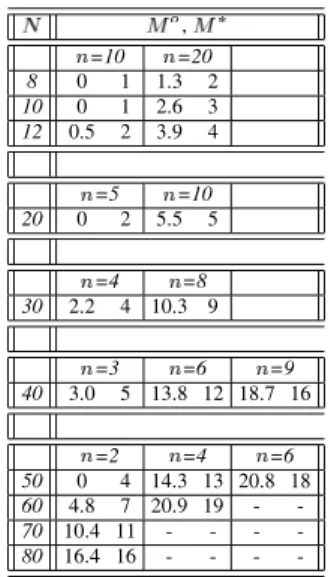
TABLE II

COMPARISON OF OPTIMUM VALUES OF FOR VARIOUS AND ,

CALCULATED FROMMGAPPROXIMATION( )AND FROMMC ( ).

, =10 =20 8 0 1 1.3 2 10 0 1 2.6 3 12 0.5 2 3.9 4 =5 =10 20 0 2 5.5 5 =4 =8 30 2.2 4 10.3 9 =3 =6 =9 40 3.0 5 13.8 12 18.7 16 =2 =4 =6 50 0 4 14.3 13 20.8 18 60 4.8 7 20.9 19 - -70 10.4 11 - - - -80 16.4 16 - - -

-In Table II we compare the results for the optimal obtained by: (i) Equation (3), denoted by , and (ii) by the MC model, denoted by . This table is to be read as follows: For example,

suppose and , the optimal equals (i)

, and (ii) . The approximation is quite accurate over a large range of values of and for reasonable operating conditions. In particular, it is only when the number of fresh samples ( ) is less than the number of bins ( ), for

example for , , and , that is not very

close to .

VI. TRACEDRIVENSIMULATIONS

In this section we conduct web-trace driven simulations to evaluate the performance of our algorithm under real traffic. In particular, we approximate deterministic cache replacement schemes using our randomized algorithm, and compare the per-formance of the deterministic schemes with the perper-formance of the randomized algorithm. Recall that any cache replacement algorithm is characterized by a utility function, and that each item in the cache is characterized by its sorting value, assigned by the respective utility function. The main issues we wish to understand by conducting the simulations are:

How good is the performance of the randomized algorithm ac-cording to realistic metrics like hit rate and latency? It is impor-tant to understand this because we have analyzed performance using the frequency of eviction from designated percentile bins as a metric. This metric has a strong positive correlation with realistic metrics but doesn’t directly determine them.

Our analysis in the previous sections assumes that documents retained in memory are not accessed between iterations. Clearly, in practice, this assumption can only hold with a high probabil-ity at best. We show that this is indeed the case and determine the probability that a sample retained in memory is accessed be-tween iterations.

How long do the best eviction candidates stay in the cache? If this time is very long (on average), then the randomized scheme

(6)

would waste space on “dead” items that can only be removed by a cache flush.

Of the three items listed above, the first is clearly the most important and the other two are of lesser interest. Accordingly, the bulk of the section is devoted to the first question and the other two are addressed towards the end.

A. Deterministic Replacement Algorithms

Using our randomization technique, we shall approximate the following two deterministic algorithms: LRU and GD-Hyb. GD-Hyb is a combination of the GD-Size [2] and the Hybrid [13] algorithms. LRU is chosen because it is the standard cache replacement algorithm. GD-Hyb is chosen to represent the class of new algorithms that base their document replacement policy not only on recentness of use, but also on the size of a document, the cost to fetch it from the server, and its frequency of use. We briefly describe the details of the deterministic algorithms men-tioned above.

1. LRU.The utility function assigns to each document the most recent time that the document was accessed.

2. Hybrid [13].The utility function assigns eviction values to documents according to the formula

where is an estimate of the latency for connecting with the corresponding server, is an estimate of the bandwidth between the proxy cache and the corresponding server, is the number of times the document has been requested since it entered the cache (frequency of use), is the size of the document, and , are weights8_{. Hybrid evicts the document with the smallest}

value of .

3. GD-Size [2].Whenever there is a request for a document, the utility function adds the reciprocal of the document’s size to the currently minimum eviction value among all the documents in the cache, and assigns the result to the document. Thus, the eviction value for document is given by

in cache

Note that the quantity in cache is increasing in time and it is used to take into account the recentness of a document. Indeed, since whenever a document is accessed its eviction value is increased by the currently minimum eviction value, the most recently used documents tent to have larger eviction values. GD-Size evicts the document with the smallest value of .

4. GD-Hybuses the utility function of Hybrid in place of the quantity in the utility function of GD-Size. Thus, its utility function is as follows:

where

We shall refer to the randomized versions of LRU and GD-Hyb as RLRU and GD-Hyb respectively. Note that the RGD-Hyb algorithm uses the among the samples, and not the global among all documents in the cache.

In the simulations we use the same weights as in [13].

So far we have described the utility functions of some de-terministic replacement algorithms. Next, we comment on the implementation requirements of those schemes. Recall that the randomized algorithm requires no data structures to be imple-mented, irrespectively of which deterministic scheme it approx-imates.

LRU can be implemented with a linked list that maintains the order in which the cached documents were accessed so far. This is due to the “monotonicity” property of its utility func-tion; whenever a document is accessed, it is the most recently used. Thus, it should be inserted at the bottom of the list and the least recently used document always resides at the top of the list. However, most algorithms, including those that have the best performance, lack the monotonicity property and they re-quire to search all documents to find which to evict. To reduce computation overhead, they must use a priority queue to drop the

search cost to , where is the number of documents

in the cache. In particular, Hybrid, GD-Size, and GD-Hyb must use a priority queue.

The authors in [6] propose an algorithm called LRV (Lowest Relative Value). This algorithm uses a utility function that is based on statistical parameters collected by the server. By sepa-rating the cached documents into different queues according to the number of times they are accessed, or their relative size, and by taking into account within a queue only time locality, the al-gorithm maintains the monotonicity property of LRUwithina queue. LRV evicts the best among the documents residing at the head of these queues. Thus, the scheme can be implemented with a constant number of linked lists, and finds an eviction can-didate in constant time. However, its performance is inferior to algorithms like GD-Size [2]. Also, the cost of maintaining all these linked lists is still high.

The best cache replacement algorithm is in essence the one with the best utility function. In this paper we don’t seek for the best utility function. Instead, we propose a low cost, high performance, robust algorithm that treats all the different utility functions in a unified way. We show that the randomized ver-sion of any scheme, regardless of the utility function it uses, can perform as well as the non-random scheme, without the need to maintain any data structures.

B. Web Traces

The traces we use are taken from Virginia University, Boston University, and National Laboratory for Applied Network Re-search (NLANR). In particular:

The Virginia [12] trace consists of every URL request ap-pearing on the Computer Science Department backbone of Vir-ginia University with a client inside the department, naming any server in the world. The trace was taken for a 37 day period in September and October 1995 representing around 54000 re-quests. There are no latency data on that trace thus it can not be used to evaluate RGD-Hyb.

Boston[3] traces consist of two sets. They record all HTTP re-quests originating from 32 workstations. The first was collected in January 1995 and consists of around 18000 requests. The second was collected in February 1995 and consists of around 110000 requests. Both contain latency data.

(7)

0 2 4 6 8 10 12 14 16 18 20 45 50 55 60 65 70 75 80 85 90

% relative cache size

% hit rate NLANR Trace 09/23/00 non−random(LRU)=solid random(N=30,M=5)=cross random(N=8,M=2)=circle random(N=3,M=1)=diamond random(RR)=square non−random(LRU)=solid random(N=30,M=5)=cross random(N=8,M=2)=circle random(N=3,M=1)=diamond random(RR)=square

Fig. 6. Hit rate comparison between LRU and RLRU.

The NLANR [14] traces consist of seven daily sets, with around 300000 requests each. The daily traces were recorded from the 22nd to 28th of September 20009_{. All of them contain}

latency data.

We only simulate requests with a known reply size.

C. Results

The performance criteria used are three:

(i) the hit rate (HR), which is the fraction of client-requested URLs returned by the proxy cache,

(ii) the byte hit rate (BHR), which is the fraction of client re-quested bytes returned by the proxy cache, and

(iii) the latency reduction (LR), which is the reduction of the waiting time of the user from the time the request is made till the time the document is fetched to the terminal (download latency), over the sum of all download latencies.

For each trace, HR, BHR, and LR are calculated for a cache of infinite size. Then, they are calculated for a cache of size , and of the maximum size required to avoid any evictions. This size is around 500MB, 900MB, and 2GB for Virginia, Boston, and each daily NLANR trace respectively. All the traces give similar results. Since the NLANR traces consist of more requests, are more recent, and contain latency data, we only present simulation results from those traces.

Figure 6 and 7 present the ratio of HR of various schemes over the HR achieved by an infinite cache. The former figure compares LRU to RLRU, and the later GD-Hyb to RGD-Hyb. In Figure 6, RLRU nearly matches LRU for and as small as 8 and 2 respectively. In Figure 7, RGD-Hyb requires 30 sam-ples and a memory of 5 to closely approximate GD-Hyb. The performance of GD-Hyb is superior to LRU. Indeed, GD-Hyb achieves around 100% of the infinite cache performance while LRU achieves below 90%. Note that RR’s performance is 15% worse than GD-Hyb’s.

NLANR traces consist of daily traces from many sites; the traces we used are from the PA site.

0 2 4 6 8 10 12 14 16 18 20 40 50 60 70 80 90 100

% hit rate

NLANR Trace 09/23/00

non−random(GD−Hyb)=solid random(N=30,M=5)=cross random(N=8,M=2)=circle random(N=3,M=1)=diamond random(RR)=square non−random(GD−Hyb)=solid random(N=30,M=5)=cross random(N=8,M=2)=circle random(N=3,M=1)=diamond random(RR)=square

Fig. 7. Hit rate comparison between GD-Hyb and RGD-Hyb.

0 2 4 6 8 10 12 14 16 18 20 50 55 60 65 70 75 80 85 90 95

% hit rate NLANR Trace 09/28/00 non−random(LRU)=solid random(N=30,M=5)=cross random(N=8,M=2)=circle random(N=3,M=1)=diamond random(RR)=square non−random(LRU)=solid random(N=30,M=5)=cross random(N=8,M=2)=circle random(N=3,M=1)=diamond random(RR)=square

Fig. 8. Hit rate comparison between LRU and RLRU.

Similar results are obtained from all traces. As a second ex-ample, Figure 8 and 9 plot the HR achieved by LRU,LRLU and GD-Hyb, RGD-Hyb respectively, using another daily NLANR trace. Again RLRU nearly matches LRU for and as small as 8 and 2 respectively, and GD-Hyb requires 30 samples and a memory of 5 to closely approximate GD-Hyb.

Figure 10 and 11 present the ratio of BHR of various schemes over the BHR achieved by an infinite cache. The former figure compares LRU to RLRU, and the later GD-Hyb to RGD-Hyb. The randomized algorithm works well in respect to BHR, re-quiring and to be as low as 3 and 1.

Note that RGD-Hyb performs better than GD-Hyb for small cache sizes and more importantly, LRU performs as good as GD-Hyb. Actually, for some of the traces LRU performed slightly better than GD-Hyb. This somewhat unexpected re-sult is caused because GD-Hyb makes relatively poor choices

(8)

0 2 4 6 8 10 12 14 16 18 20 50 55 60 65 70 75 80 85 90 95 100

% hit rate

Fig. 9. Hit rate comparison between GD-Hyb and RGD-Hyb.

0 2 4 6 8 10 12 14 16 18 20 65 70 75 80 85 90 95

% byte hit rate

NLANR Trace 09/28/00 non−random(LRU)=solid random(N=30,M=5)=cross random(N=8,M=2)=circle random(N=3,M=1)=diamond random(RR)=square non−random(LRU)=solid random(N=30,M=5)=cross random(N=8,M=2)=circle random(N=3,M=1)=diamond random(RR)=square

Fig. 10. Byte Hit rate comparison between LRU and RLRU.

in terms of BHR by design, since it has a strong bias against large size documents even when these documents are popular. This suboptimal performance of GD-Hyb is inherited from SIZE [12] and Hybrid [13] and could be removed by fine-tuning. All the three schemes trade in HR for BHR10_.

Figure 12 and 13 present the ratio of LR of various schemes over the LR achieved by an infinite cache. The former figure compares LRU to RLRU, and the later GD-Hyb to RGD-Hyb. In Figure 12, RLRU nearly matches LRU for and as small as 3 and 1 respectively. In Figure 13, it suffices for and to be equal to 8 and 2 respectively for RGD-Hyb to perform very well.

Recently, an algorithm called GreedyDual* has been proposed [5], that achieves superior HRandBHR when compared to other web cache replacement policies. 0 2 4 6 8 10 12 14 16 18 20 45 50 55 60 65 70 75 80 85 90 95

% byte hit rate

Fig. 11. Byte Hit rate comparison between GD-Hyb and RGD-Hyb.

0 2 4 6 8 10 12 14 16 18 20 50 55 60 65 70 75 80 85 90 95

% reduced latency NLANR Trace 09/23/00 non−random(LRU)=solid random(N=30,M=5)=cross random(N=8,M=2)=circle random(N=3,M=1)=diamond random(RR)=square non−random(LRU)=solid random(N=30,M=5)=cross random(N=8,M=2)=circle random(N=3,M=1)=diamond random(RR)=square

Fig. 12. Latency reduction comparison between LRU and RLRU.

From the figures above, it is evident that the randomized ver-sions of the schemes can perform competitively with very small number of samples and memory. One would expect to require more samples and memory to get such good performance. How-ever, since all the online cache replacement schemes rely on heuristics to predict future requests, it is not necessary to ex-actly mimic their behavior in order to achieve high performance. Instead, it usually suffices to evict a document that is within a reasonable distance from the least useful document.

There are two more issues to be addressed. First, we wish to estimate the probability that documents retained in memory are accessed between iterations. This event very much depends on the request patterns and is hard to analyze exactly. Instead, we use the simulations to estimate the probability of occurring. Thus, we change the eviction value of a document retained in

(9)

0 2 4 6 8 10 12 14 16 18 20 50 55 60 65 70 75 80 85 90 95 100

% reduced latency

non−random(GD−Hyb)=solid random(N=30,M=5)=cross random(N=8,M=2)=circle random(N=3,M=1)=diamond random(RR)=square

Fig. 13. Latency reduction comparison between GD-Hyb and RGD-Hyb.

memory whenever it is accessed between iterations, which dete-riorates its value as an eviction candidate. Also, we don’t obtain a new, potentially better, sample. Despite the above, the perfor-mance is not degraded. The reason is that our policy for retain-ing samples in memory deliberately chooses the best eviction candidates. Therefore, the probability that they are accessed is very small. In particular, it is less than in our simulations. Second, we wish to verify that the randomized versions of the schemes do not produce dead documents. Due to the sampling procedure, the number of sampling times that a document is not chosen follows a geometric distribution with parameter roughly equal to over the total number of documents in the cache. This is around 1/100 in our simulations. Hence, the probability that the best ones are never chosen is zero, and the best ones are chosen once every 100 sampling times or so.

VII. CONCLUSIONS

In this work we have introduced a randomized algorithm for approximating any existing web-cache replacement scheme. We find that carrying a small amount of information regarding good samples from one iteration to the next, leads to a dramatic im-provement in performance. By a judicious choice of parameters (the total number of samples, , and the number of good sam-ples, , retained from one iteration to the next) we find that any replacement scheme can be approximated as closely as desired.

Trace-driven simulations show that and suffice

in practice.

High performance deterministic algorithms require a prior-ity queue or multiple linked lists in order to reduce seek time.

Further, most of these algorithms spend time

when-ever there is an access to a document to keep the data struc-ture updated. From an implementation point of view this is much more complex than avoiding the use of any data struc-ture and just randomly sampling 6 documents and remembering

2 ( ) whenever a document is to beevicted.

In general, our scheme can be used efficiently whenever there is a large population of objects from which the “best” is to be

chosen according to some utility function.

VIII. ACKNOWLEDGMENTS

We thank Dawson Engler for early conversations regarding cache replacement schemes, and A.J. Ganesh for fruitful dis-cussions regarding the martingale argument.

REFERENCES

[1] M. Abrams, C.R. Standbridge, G. Abdulla, S. Williams and E.A. Fox, “Caching Proxies: Limitations and Potentials”,WWW-4, Boston, Decem-ber, 1995.

[2] P. Cao and S. Irani, “Cost-Aware WWW Proxy Caching Algorithms”, In proceedings of theUSENIX Symposium on Internet Technologies and Sys-tems, Monterey, CA, Dec. 1997.

[3] C.R. Cunba, A. Bestavros, M.E. Crovella, “Characteristics of WWW Client-based Traces”, BU-CS-96-010, Boston University.

[4] R. Durrett,Probability: Theory and Examples, Duxbury Press, 2nd edi-tion, 1996.

[5] S. Jin and A. Bestavros, “GreedyDual* Web Caching Algorithm: Exploit-ing the Two Sources of Temporal Locality in Web Request Streams”, In Proceedings of the5th International Web Caching and Content Delivery Workshop, Lisbon, Portugal, May 2000.

[6] L. Rizzo and L. Vicisano, “Replacement Policies for a Proxy Cache”, IEEE/ACM Transactions On Networking, Vol. 8, No. 2, April 2000. [7] R. Motwani and P. Raghavan,Randomized Algorithms, Cambridge

Uni-versity Press, 1995.

[8] J. Norris,Markov Chains, Cambridge University Press, 1997.

[9] K. Psounis, B. Prabhakar, D. Engler, “A Randomized Cache Replacement Scheme Approximating LRU”,34th Annual Conference on Information Sciences and Systems, March 15-17, Princeton University.

[10] K. Psounis, B. Prabhakar, “A Randomized Web-Cache Replacement Scheme”, CSL Technical Report No: CSL-TR-00-805, Revision 1, De-cember 2000, Stanford University.

[11] A. Silberschatz and P. Galvin,Operating System Concepts, Fifth Edition, Addison Wesley Longman, 1997.

[12] S. Williams, M. Abrams, C.R. Standbridge, G. Abdulla and E.A. Fox, “Re-moval Policies in Network Caches for World-Wide Web Documents”, In Proceedings of theACM Sigcomm96, August, 1996, Stanford University. [13] R. Wooster and M. Abrams, “Proxy Caching that Estimates Edge Load

Delays”, In the6th International World Wide Web Conference, April 7-11, 1997, Santa Clara, CA.