Management of productivity, environmental effects and profitability
of shellfish aquaculture
—
the Farm Aquaculture Resource
Management (FARM) model
J.G. Ferreira
a,⁎
, A.J.S. Hawkins
b, S.B. Bricker
caIMAR—Institute of Marine Research, Centre for Ecological Modelling, IMAR–DCEA, Fac. Ciencias e Tecnologia, Qta Torre,
2829-516 Monte de Caparica, Portugal
bPlymouth Marine Laboratory, The Hoe, Plymouth PL1 3DH, Devon, United Kingdom
cNOAA—National Ocean Service, National Centers for Coastal Ocean Science, 1305 East West Highway, Silver Spring, MD 20910, USA Received 24 August 2006; received in revised form 29 October 2006; accepted 6 December 2006
Abstract
This paper describes a model for assessment of coastal and offshore shellfish aquaculture at the farm-scale. The Farm Aquaculture Resource Management (FARM) model is directed both at the farmer and the regulator, and has three main uses: (i) prospective analyses of culture location and species selection; (ii) ecological and economic optimisation of culture practice, such as timing and sizes for seeding and harvesting, densities and spatial distributions (iii) environmental assessment of farm-related eutrophication effects (including mitigation).
The modelling framework applies a combination of physical and biogeochemical models, bivalve growth models and screening models for determining shellfish production and for eutrophication assessment. FARM currently simulates the above interrelations for five bivalve species: the Pacific oysterCrassostrea gigas, the blue musselMytilus edulis, the Manila clamTapes phillipinarum, the cockleCerastoderma eduleand the Chinese scallopChlamys farreri. Shellfish species combinations (i.e. polyculture) may also be modelled.
We present results of several case studies showing how farm location and practice may result in significant (up to 100%) differences in output (production). Changes in seed density clearly affect output, but (i) the average physical production decreases at higher densities and reduces profitability; and (ii) gains may additionally be offset by environmental costs, e.g. unacceptable reductions in dissolved oxygen. FARM was used for application of a Cobb–Douglas function in order to screen for economically optimal production: we show how marginal analysis can be used to determine stocking density. Our final case studies examine interactions between shellfish aquaculture and eutrophication, by applying a subset of the ASSETS methodology. We provide a tool for screening various water quality impacts, and examine the mass balance of nutrients within a 6000 m2oyster farm. An integrated analysis of revenue sources indicates that about 100% extra income could be obtained by emissions trading, since shellfish farms are nutrient sinks. FARM thus provides a valuation methodology useful for integrated nutrient management in coastal regions.
The model has been implemented as a web-based client–server application and is available athttp://www.farmscale.org/. © 2006 Elsevier B.V. All rights reserved.
Keywords:Shellfish carrying capacity; Screening model; Farm-scale management; Aquaculture; Eutrophication; Nutrient trading
⁎Corresponding author. Fax: +44 20 7691 7827.
E-mail address:joao@hoomi.com(J.G. Ferreira).
0044-8486/$ - see front matter © 2006 Elsevier B.V. All rights reserved. doi:10.1016/j.aquaculture.2006.12.017
1. Introduction
Shellfish aquaculture is of great importance world-wide, with production increasing at an average of
7.8% per annum over the last 30 years (FAO, 2004),
stimulated by market demand and by legislative initiatives such as the proposed U.S. Offshore Aqua-culture Act (NOAA, 2006). The potential diversity of cultivated species (e.g. oysters, mussels, scallops, clams), each with different environmental adaptations, the pressure towards optimising species combinations within polyculture and integrated multi-trophic aqua-culture (IMTA) (Fang et al., 1996; Nunes et al., 2003; Neoria et al., 2004) and the technical developments that
increasingly afford suspended “pelagic” habitats in
addition to bottom culture together provide significant challenges to sustainable management. These chal-lenges are made more acute by pressures for further expansion in an industry whose production has doubled every 15 years in the recent past.
Assessments of sustainable mariculture in general and shellfish culture in particular are conditioned by different definitions of carrying capacity, which may be regarded as physical, production, ecological and
social (Inglis et al., 2000). These are themselves
modulated by scaling, usually considered to be either system scale (bay, estuary or sub-units thereof), or
local scale (farm). McKindsey et al. (2006)
pro-vide a critical review of methods, including models, used for evaluating these various types of carrying capacity.
System-scale management of shellfish aquaculture requires a top-down assessment of carrying capacity, and has many similarities to any other large-scale plan for optimising the multiple uses of goods and ser-vices. Models (of varying complexity) that address
system-scale issues include those of Carver and
Mallet (1990), Raillard and Ménesguen (1994),
Ferreira et al. (1998), Gangnery et al. (2001) and
Nunes et al. (2003). At the local scale, the evaluation of potential fish aquaculture sites has also been
supported by models such as DEPOMOD (Cromey
et al., 2002) and MOM (Stigebrandt et al., 2004), but there are very few models for analysis of shellfish
farms. Most recently,Bacher et al. (2003)combined a
hydrodynamic model, measured data on food con-centration and the simulation of individual shellfish growth to optimise density according to biological production alone.
Environmental influences of bivalve filter-feeders
have been discussed by many authors (e.g. Cloern,
1982; Gerritsen et al., 1994; Lucas et al., 1999), and are
most likely to be seen in systems dominated by aquaculture (Nobre et al., 2005). Effects may include a
top-down control of eutrophication symptoms (sensu
Bricker et al., 2003), when selective filtration may
additionally influence the composition of phytoplankton species (Shumway et al., 1985; Bougrier et al., 1997), as well as consequences for water column biogeochemistry
(Souchu et al., 2001). On the other hand, causative
factors of coastal eutrophication, such as increased nitrogen and phosphorus loading, may by virtue of higher primary production be associated with enhanced shellfish growth (Weiss et al., 2002).
This paper presents a modelling approach for the analysis of farm-scale aquaculture, applicable to a range of widely cultivated shellfish species. The Farm Aquaculture Resource Management (FARM) model is targeted at farmers and managers. Whilst distilled from more complex models, FARM has therefore been designed as a simplified screening model, using a reduced parameter set, based on data which are easily available. The main objectives of this work are:
(i) to develop a model for determining sustaina-ble carrying capacity in shellfish aquaculture farms;
(ii) to optimise culture practice, such as timing and sizes for seeding and harvesting, densities and spatial distributions, both in terms of total production and economic returns;
(iii) to assess the role of shellfish farms in eutrophi-cation control and emissions trading.
2. Methods
2.1. Conceptualisation
The FARM model simulates processes at the farm scale (about 100–1000 m), considering advective water flow and the corresponding transport of relevant water properties. These properties include the total concentration of suspended particulate matter (TPM), separate components of that suspended food resource which include living phytoplankton organics as
distinct from all remaining “detrital” organics, and
dissolved materials which include ammonia and dissolved oxygen (DO). The general layout for the
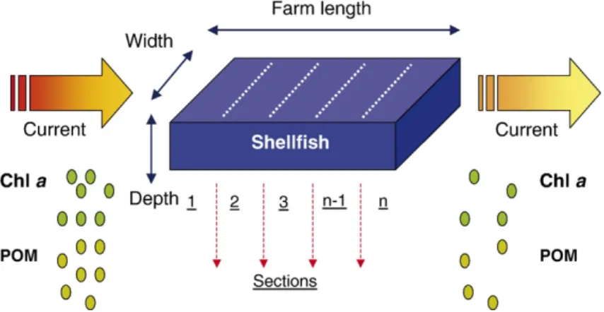
model is shown in Fig. 1, and is applicable to
sus-pended culture from rafts or longlines as well as to bottom culture. Horizontal water transport is simulated
using a one-dimensional model, following e.g.Bacher
et al. (2003), to which vertical transport is added for suspended culture.
Requirements for input data have been reduced to a minimum, since the model is aimed at the shellfish farming community and local managers in different parts of the world. Model inputs may be grouped into data on (i) farm layout, dimensions, species composition and stocking densities; (ii) suspended food entering the farm; and (iii) environmental parameters.
FARM integrates a combination of physical and biogeochemical models, shellfish growth models and screening models for determining production and for eutrophication assessment. These compo-nents are illustrated in Fig. 2and described in detail below.
2.2. Physical and biogeochemical models
The general formulation used in FARM for model-ling pelagic state variables in a suspended culture system is given in Eq. (1):
AC At ¼−u AC Ax−w AC Az þfðC; X i¼1 i¼m nigiÞ ð1Þ where:
C concentration of resource (phytoplankton,
POM, TPM)
Fig. 2. Conceptual scheme of the various components of the FARM model. The model core is within the dotted rectangle, the two screening models are external.
t time
u mean horizontal water velocity normal to farm
cross-section
x farm section length
w fall velocity of suspended particles
z farm section depth
m number of weight classes in the population
ni number of cultivated shellfish in weight classi
γi growth functions for individual shellfish in
weight classi
A mean unidirectional horizontal flow is considered, based on the current speed and on the farm dimensions, which may be defined as a series of contiguous sections or boxes, both to allow the analysis of different culture layouts and to minimise numerical errors. The model is designed to be applied over a time-scale which encompasses the range of cultivation periods observed in shellfish aquaculture, which may range from a few months to 2–3 years. Given the restriction imposed by the spatial scale of simulations for small farms, the specification of a high number of sections conditions the model time step, which is automatically determined to satisfy the Courant condition for stability.
Vertical fluxes for particulates are calculated for farms that implement suspended culture. At every time step, FARM calculates the dynamic viscosity based on the water temperature and salinity, and uses the Stokes equation to determine the fall velocity and particle deposition, taking different grain sizes into account followingFerreira et al. (1998). For farms implementing bottom or near-bottom culture involving benthic dredging or trestle systems, the deposition term is not considered.
The third term in Eq. (1) is a general representation of sinks and sources associated to shellfish growth—this term may be a sink for e.g. dissolved oxygen or chlorophyll a, a source for e.g. excreted ammonia, or both for e.g. POM and other particulate matter, which may be removed during ingestion and returned to the system as pseudofaeces and faeces.
2.3. Shellfish models
The growth of five different bivalve species is simulated in FARM (Table 1). Different types of models have been used, but all have in common the simulation
of individual growth. The models for clams (Solidoro
et al., 2000), Chinese scallop (Hawkins et al., 2002) and cockles (Rueda et al., 2005) are fully described in the literature. The models for mussels and oysters build
upon that described for the Chinese scallop (Hawkins
et al., 2002), and which has since been developed into a generic model structure for the dynamic simulation of feeding, metabolism and growth in different species of suspension-feeding bivalve shellfish, calibrated and validated for these and other species cultured at contrasting sites throughout Europe (Hawkins et al., in preparation).
To simulate the biomass production of market-size organisms, each model of shellfish growth is integrated in a population dynamics framework using
well-established equations (e.g. Nunes et al., 2003; Nobre
et al., 2005). Growth rates for individual shellfish are calculated on the basis of food supply and environ-mental parameters supplied by the physical and bio-geochemical models. Shellfish mortality is also required as a driver for the population dynamics model. Average natural mortalities were estimated from data describing cultivation practices in Europe and China, and which are implemented in FARM
(Fig. 2) according to established environmental
stressors that include high temperatures, low salinities
and low concentrations of dissolved oxygen (Hawkins
and Bayne, 1992).
2.4. Screening models
Two types of screening models were incorporated in FARM. These are described below:
2.4.1. Aquaculture production
The outputs of the FARM model enable a detailed analysis of the production of market-sized animals for each cultivated species. Multiple simulations with increasing shellfish density yield a curve representing the total physical product (TPP) in tons total fresh weight (TFW). This is a Cobb–Douglas production
Table 1
Shellfish species and models used in FARM Species Common
name
Reference/model Model type
Crassostrea gigas Pacific oyster Hawkins et al. (in preparation); ShellSIM Ecophysiological
Mytilus edulis Blue mussel Hawkins et al. (in preparation); ShellSIM Ecophysiological Tapes phillipinarum Manila clam Solidoro et al. (2000) Bioenergetic Chlamys farreri Chinese scallop Hawkins et al. (2002) Ecophysiological Cerastoderma edule
Cockle Rueda et al. (2005); COCO
function (e.g. McCausland et al., 2006) of the form given in Eq. (2):
Y ¼fðx1;jx2;x3; N xnÞ ð2Þ
where:
Y output of harvestable shellfish
x1 initial stocking density of seed, considered the
only variable input
x2−xn other inputs, considered to be held constant
The model calculates the average physical produc-tion (APP) after each run (Eq. (3)):
APPx1¼
TPP
x1 ð
3Þ and the first-order derivative of the production function provides the marginal physical product (MPP). For cons-tant input unit costPxand output unit pricePy, the farmer's
profit will be maximised when the value of the marginal product (VMP) equalsPx, VMP may be defined as:
VMP¼MPPdPy¼Px ð4Þ
making it possible to determine the MPP for profit maximisation according toJolly and Clonts (1993). The validity of this approach, which is based on marginal principles, additionally assumes that (i) inputs are unlimited, (ii) input purchases and output sales are made in a perfectly competitive market situation, (iii) the farm is a small production system which sells only this product, and (iv) seed is the only variable input, such that lease, labour etc. are fixed costs.
The FARM model also calculates the equivalent APP expressed as individuals, providing an indicator of the capacity of the farm to produce harvestable animals. 2.4.2. Eutrophication assessment
To evaluate the effects of a shellfish farm with respect to eutrophication, the Assessment of Estuarine Trophic
Status (ASSETS) model (Bricker et al., 2003) was
adapted for use at the local scale. This model, which extends the US National Eutrophication Assessment
(NEEA) methodology (Bricker et al., 1999), has been
applied at the system scale in many estuaries and coastal
bays in the US, EU and Asia (e.g.Nobre et al., 2005;
Ferreira et al., 2007; NOAA/IMAR, 2006).
With reference to the ASSETS model, the farming of filter-feeding bivalves in suspended culture may have positive impacts by reducing primary symptoms of eutrophication such as elevated chlorophylla(e.g.Newell,
2004), with an associated favourable effect on the
secondary symptom dissolved oxygen, although the
shellfish are themselves a sink for DO. In parallel, the removal of TPM and POM due to feeding, and the consolidation of suspended particles into larger (up to 40×) and more rapidly sedimenting composites as faeces and pseudofaeces (e.g.Giles and Pilditch, 2004; Newell, 2004), may promote increased water clarity, leading to a recovery in submerged aquatic vegetation (SAV). Chla, macroalgae, SAV loss, DO and harmful algae are the eutrophication symptoms considered in the ASSETS determination of State(Overall Eutrophic Condition—OEC). In the present
FARM model, only Chl a and DO are considered, and
aspects of the assessment related to weighting of spatial coverage and frequency of occurrence are not included. Conceptually, the various farm sections are equivalent to the ASSETS salinity zones, and the level of expression (Sl)
values for Chlaand DO are obtained by integration over the total farm area, using Eqs. (5) and (6) respectively. Sl¼ Xn 1 As Af El ð5Þ where:
As surface area of farm section
Af total farm surface area
El expression value in each section
n number of farm sections
and
Sl¼max El n
1 ð6Þ
Eq. (6) selects the highest level of expression of the ASSETS secondary symptom DO, in keeping with the precautionary nature of the assessment method. The standard OEC decision matrix (Bricker et al., 2003) is used to derive the final grade for State. ThePressure
and Response components within ASSETS are not
applicable at the farm scale.
2.5. Implementation, validation and sensitivity analysis 2.5.1. Implementation
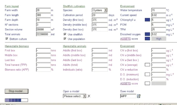
FARM has been implemented as a client–server application, using an object-oriented approach, and is
available at http://www.farmscale.org/. The model
interface is illustrated inFig. 3, and allows the user to: (i) define farm dimensions, types and durations of
cultivation;
(ii) define environmental variables (e.g. Chla, POM, TPM, O2);
Inputs for environmental variables may be derived from field data or from larger scale models. If a value is not entered for dissolved oxygen, the model automatically calculates it as 100% dissolved oxygen saturation based on temperature and salinity (afterBenson and Krause, 1984). 2.5.2. Validation
Various parts of the FARM model were developed
and tested in PowerSim™, Stella™, C++ and
FOR-TRAN. Each of the individual shellfish growth models has been validated under culture conditions (refer above
andTable 1). Many of the functions used in FARM have
been previously used in studies of system-scale carrying capacity, validated for systems in Europe (Ferreira et al., 1998; Nobre et al., 2005) and China (Nunes et al., 2003). Nunes et al. (ibid) calculated a bay-wide production of about 45,000TFW during the first year that the Chinese scallopChlamys farreriwas cultivated in Sanggou Bay, N.E. China; later years have superimposed annual cohorts, resulting in larger harvests (6 year mean = 59,868TFW y−1). FARM was run for a 1ha (500 m × 20 m) farm using identical seed densities and the results scaled up to 34 km2, which is the total cultivation area in Sanggou Bay. The
scaled-up TPP was 42,160TFW y−1, representing about
94% of the system-scale model results, and which appears acceptable. FARM is expected to predict lower yields due
to depletion effects, since ecosystem-scale models calculate carrying capacity within larger boxes, potentially neglect-ing resource scarcity at the farm-scale.
2.5.3. Sensitivity analysis
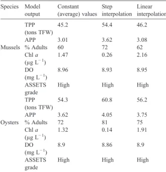
The publicly available version of FARM presently uses constant user-defined forcing for water tempera-ture, Chla, POM and TPM. In nature, all of these vary seasonally. Therefore, time-series data (Fig. 4) available
Fig. 3. FARM screenshot.
Fig. 4. Time series for sensitivity analysis to constant or variable environmental forcing. Data were collected as part of the SMILE project (IMAR/PML/CSIR/DARDNI, 2006).
for northern Irish sea loughs (IMAR/PML/CSIR/
DARDNI, 2006) were used to force the model to
explore the sensitivity of outputs to variable inputs, over a 210 day cultivation period.
The model outputs for three different cases are shown
in Table 2, for culture of both the blue mussel and
Pacific oyster. For the runs with constant forcing we used the annually averaged data, and additionally tested using stepwise and linear interpolation of the data series. There were small differences in almost all the outputs when the three forcing approaches are compared. However, the maximum difference in TPP between runs using average values and linear interpolation was no more than 3%. Larger differences of up to 20% in mussels and 12% in oysters were observed between step interpolation and both the average and linear runs. This was probably because step interpolation forces plateaus of high or low values over long periods, which will have pronounced effects on production, particularly during periods such as the spring bloom (Fig. 4), when there are steep gradients in the chlorophyll data. An ANOVA for the three data sets indicates that the results for TPP, APP,
% adults, Chl a and DO are indistinguishable, with
F= 0.028 (Pb0.97) for mussels andF= 0.009 (Pb0.99)
for oysters (criticalFvalue forPb0.05 isN3.88).
Further tests were also carried out by comparing outputs for mussels and oysters using the averaged and linearly interpolated data for 5 different current speeds, ranging from 0.01 m s−1to 0.5 m s−1. All other input data were as in the previous example. An ANOVA applied to the output pairs also suggests that statistical differences are not significant for either mussels (F= 0.04) or oysters (F= 0.05, Pb0.1≥3.46 for both
species). Finally, similar tests were carried out using the average of data collected at seven sampling stations monthly over one year from 1999 to 2000 in Sanggou Bay, China, as described for the SPEAR project athttp://
www.biaoqiang.org/. For the Chinese scallopChlamys
farreri, comparisons showed that TPP and APP were
identical using averaged and linearly interpolated environmental forcing.
Overall, the comparisons for averaged and time-varying data suggest that outputs using constant forcing are sufficiently accurate for the purposes of this type of screening model.
3. Results and discussion
A series of potential applications of the FARM model are reviewed below. These include: (i) prospective analyses of culture location and species selection; (ii) optimisation of culture practice, including effects of the times of seeding and harvesting, shellfish densities and spatial distributions on both the total production and economic returns; and (iii) environmental assessment of farm-related eutrophication effects (including mitiga-tion). The example case studies reported have been prepared using realistic model input data drawn from a variety of cultivated coastal systems. The stocking densities selected fall within the ranges cited byBacher et al. (2003).
3.1. Example applications 3.1.1. Farm location
Table 3 shows an example for three potential farm
locations, considering areas with fast (0.5 m s−1), medium (0.1 m s−1) and slow (0.02 m s−1) current speeds. All other environmental variables and initial stocking density are kept constant. The model was applied for bottom culture of the oysterC. gigasover a short cultivation period of 45 days. Modelled responses
for TPP (simulated as TFW), APP and final mean Chla
are hyperbolic, and at slow current speeds show greater food depletion and less efficient production, reflected in an APP which is 50% lower than at other siting scenarios.
Table 2
Sensitivity analysis to annual cycle of chlorophylla, POM, TPM and water temperature⁎ Species Model output Constant (average) values Step interpolation Linear interpolation TPP (tons TFW) 45.2 54.4 46.2 APP 3.01 3.62 3.08 Mussels % Adults 60 72 62 Chla (μg L−1) 1.47 0.26 2.16 DO (mg L−1) 8.96 8.93 8.95 ASSETS grade
High High High
TPP (tons TFW) 54.3 60.8 56.2 APP 3.62 4.05 3.75 Oysters % Adults 72 81 75 Chla (μg L−1) 1.32 0.14 1.91 DO (mg L−1) 8.9 8.86 8.9 ASSETS grade
High High High
⁎Model runs: suspended culture for 210 days, 50 animals m−3, current speed = 0.02 m s−1. For constant values: water temperature = 9.64 °C; Chla= 1.63μg L−1; POM = 2.25 mg L−1; TPM = 7. 31 mg L−1; for interpolation data points seeFig. 4.
There is no significant difference in the production simulated at sites with fast and medium current speeds, but the latter have an environmental advantage with
respect to Chl a reduction. That advantage may,
however, be offset by an increase in local shellfish biodeposit production. Those deposits will have a smaller albeit more concentrated benthic footprint, since there will be lower particle dispersion at medium
current speeds: 0.5 m s−1is often considered a threshold between depositional and dispersive areas. It is important to bear in mind, however, that advective components transversal to the main flow direction are neglected in the present version of the FARM model. This approximation is reasonable both with respect to siting criteria for shellfish farms, which include the prevailing water currents, and in order to retain the simplicity of input data. However, the contribution of perpendicular flow components and of turbulent
diffusion may be relevant — our model may thus
underestimate resource renewal, and thus carrying capacity in absolute terms, though the relative effects of alterations in forcing functions are likely to remain unchanged.
3.1.2. Culture layout
The relative densities of shellfish in different sections of each farm may also condition the overall production. Distribution scenarios for (a) increasing density; (b) equal density; and (c) decreasing density, together with simulated consequences, are shown over three farm sections inTable 4.
Comparisons were carried out over a 45 day period, as an example of ongrowing during optimal time of year,
with a nominal current speed of 10 cm s−1, for a
standard total seed stock of 18 × 106 blue mussels in suspended culture, distributed over 9 farm sections. The number of modelled sections was increased from 3 to 9 to reduce the potential for numerical artifacts that might influence the results.
Predictions from this example indicate that higher seed densities in the first sections of the farm result in
Table 4
Culture distribution forM. edulisin suspended culture with different layouts (above the dotted line: initial conditions, with scenario changes underlined; below the line: model outputs)
Table 3
Culture siting forC. gigas(bottom culture) at locations with different current speeds (above the dotted line: initial conditions, with scenario changes underlined; below the line: model outputs)
significantly higher overall production. If growth were a simple function of food concentration, then as long as the overall biomass of seed were the same, longitudinal variations in stocking density would not lead to changes in production. However, additional release of POM from pseudofaeces and faeces produced by shellfish in upstream sections of a farm constitutes an extra source
of food for animals in downstream sections (Newell,
2004). Alternatively, and consistent with our observa-tion of higher overall producobserva-tion given higher seed densities in the first sections of the farm, then because individual growth is simulated by means of non-linear functions whereby ingestion rates and growth may
become saturated above“optimal”food concentrations
which differ between species (e.g.Hawkins et al., 2002), low seed densities and thus with lower food depletion may not maximize growth. Similarly, at lower seed densities, a greater proportion of animals will reach the largest weight classes, and which have a much lower growth efficiency (= energy deposited as growth / energy absorbed) (Nunes et al., 2003). Whilst these factors may result in better yields with increasing densities, inter-relations with current speed are all-important. For example, a 20 day model run for oyster bottom culture using slow current speeds of 1 cm s−1results in severe food depletion, with no growth in downstream sections
of the farm, such that a 14% increase in yield is instead predicted for a cultivation layout with increasing downstream density.
3.1.3. Stocking density and production screening model
Table 5 shows results for bottom culture of Pacific
oyster cultivated for 180 days at three different densities. At the low and medium densities of 25 and 100 animals m−3, respectively, the APP remains constant at 4.6. However, at the high density of 500 animals m−3, APP reduces to 2.7. Although the TPP increases from 34 tons TFW to 400 tons TFW at the highest density, the farm becomes progressively less profitable.
To obtain a production function for TPP, this simulation was extended over a range of seeding effort from 0 to 180 tons, and the results presented inTable 6. An analysis of the interactions of the resulting TPP, APP and MPP curves shows that these can be divided into three stages
(Fig. 5). In Stage I, the MPP curve is above APP, and
crosses it when the derivative of APP becomes negative. The farmer should clearly consider increasing inputs (in this case seeding density) while the APP is still increasing. Stage III begins when MPP = 0. Thereafter, TPP decreases despite increased seed input, which is clearly undesirable on a financial basis. Stage II is the region where profit is maximised. The point at which profit maximisation occurs was determined in this
example by applying Eq. (4) with Px= 0.75€ and
Py= 5€, giving an MPP = 0.15 and optimum seed input
of 90 tons TFW (density of 300 animals m−3). The maximum biological production (TPP) occurs when MPP = 0, and corresponds to a seed input of about 100 tons TFW. However, maximising biological produc-tion does not maximise profits, which are greatest at lower
Table 5
C. gigasin bottom culture with different stocking densities (above the dotted line: initial conditions, with scenario changes underlined; below the line: model outputs)
Table 6
Production and economic parameters for different seeding densities Seed (tons) TPP (tons) APP MPP VMP (€) Total revenue (k€) Total cost (k€) Profit (k€) 0 0 0.00 0.00 0.0 0 0 0 7.5 15 1.98 1.98 9.9 74 6 69 15 31 2.05 2.12 10.6 154 11 143 30 66 2.20 2.34 11.7 329 23 307 39 86 2.21 2.23 11.2 430 29 401 60 118 1.97 1.53 7.7 591 45 546 75 128 1.71 0.68 3.4 642 56 586 86 131 1.54 0.30 1.5 657 64 593 90 132 1.47 0.15 0.8 661 68 593 99 133 1.34 0.07 0.3 664 74 590 111 133 1.19 −0.02 −0.1 663 83 580 120 132 1.10 −0.07 −0.3 660 90 570 150 129 0.86 −0.10 −0.5 645 113 532 180 125 0.70 −0.12 −0.6 627 135 492 Optimal values shown in bold.
levels of input and output than those that maximise production. The profit maximising rule is based on marginal principles. Therefore, a producer who bases production decisions on average or total production and revenue principles will earn less profit than one who uses marginal analysis (Jolly and Clonts, 1993). The level of fixed cost does not influence the decision of a producer on optimal use of the variable input, since this is based on the comparison of values of Marginal Product and Marginal Input. Multiple input and output variables such as may occur under multi-species culture may also be considered by using marginal analysis, or alternative methods may be applied (e.g.Sharma et al., 1999).
FARM allows modelling of multi-species culture for different combinations of bivalves. A number of simulations with a two-species mix using various ratios of oysters and mussels did not show enhanced TPP or APP, both for constant and variable forcing. However, different species of filter-feeding shellfish feed upon different components of the suspended seston, with different maximal rates, and which occur at different seston concentrations (e.g.Hawkins and Bayne, 1992). For these reasons, it is to be expected that species composition will affect total productivity. For example,
Duarte et al. (2003)simulated the means by which total
production of shellfish could be significantly increased through spatial separation of standard seeding quantities for oysters and scallops cultured coincidentally within Sanggou Bay, China; and which appeared to result from reduced inter-specific competition. Further to which, regardless of enhancements in production alone, there may be economic advantages in combining slower-growing, higher-value species with more productive but commercially less interesting ones.
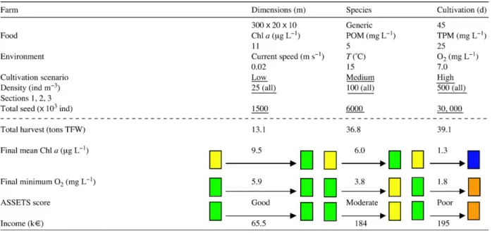
3.1.4. Eutrophication control and emissions trading Our final example provides an analysis of the interactions between shellfish culture and coastal eutrophication (Table 7). Bivalve growth was simulated over a 45 day cultivation period at three different seed densities of 25, 100 and 500 individuals m−3. As before, increasing seed density improves the final yield
Table 7
Environmental assessment—the ASSETS model (above the dotted line: initial conditions, with scenario changes underlined; below the line: model outputs)
Fig. 5. Economic analysis. Simulations carried out with C. gigas, 20 day cultivation period, 5μg L−1Chla.
(although APP is lower), but the interaction between cultivation and the ASSETS eutrophication indicators
introduces an additional “sustainability” metric for
carrying capacity assessment.
As expected, the farm with lowest shellfish density
shows the lowest food depletion, where Chl a is only
reduced by about 15%. However, DO does not fall below 6 mg L−1, resulting in an overall ASSETS score ofGood. Alternatively, the increase in density progressively leads to improved water quality as regards Chla, but the in-crease in shellfish population metabolism leads to severe reductions in DO. The ASSETS grade correspondingly shifts with increasing cultivation intensity fromModerate
at medium shellfish density to Poor at high shellfish
density. At the highest density of 500 individuals m−3, the farm area is classified as hypoxic, both using the ASSETS range (0–2 mg L−1) and the threshold ofb2.8 mg L−1
suggested by Altieri and Witman (2006). Hypoxia is
responsible for severe bivalve mortality, linked both to nutrient-related eutrophication symptoms and to benthic community respiration (e.g.Altieri and Witman, 2006). FARM allows a user to test for thresholds of low oxygen and to examine potential consequences for water quality and stock mortality.
Regulatory pressure on coastal water quality stan-dards has matched expansion pressure on shellfish aquaculture, particularly in the EU with the enactment
of the Water Framework Directive (European
Commis-sion, 2000) and the proposed Marine Strategy Directive.
TheUS Clean Water Act (CWA, 1972)and other policy
initiatives (e.g.USEPA, 2001) have also sharpened the focus on related issues. Shellfish aquaculture is widely
considered to have a positive impact, given production near the base of the trophic chain (e.g. Naylor et al.,
2000) and potential enhancements both of primary
production and biodiversity (Gibbs, 2004; McKindsey
et al., 2006). However, the environmental role of
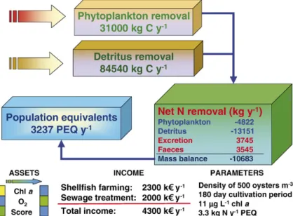
shellfish farms with respect to the control of nutrient emissions has not to our knowledge been quantitatively addressed. To assess the role of cultured shellfish on nutrient removal by means of a mass balance, FARM was run for bottom culture of oysters over a 180 day period. Fig. 6 displays the results for nitrogen, which show a net removal of about 10.7 tons y−1. A similar calculation can be carried out for phosphorus. The filtration and hence removal of particulate organic nitrogen (PON) and other organic matter by shellfish is offset by additions due to ammonia excretion and faeces. Pseudofaeces have not been included in this balance because they are rejected prior to ingestion of phytoplankton and detritus. Whilst phytoplankton primary production directly removes dissolved available inorganic nitrogen (DAIN) from the water column, the PON present in suspended particulates may originate from a variety of sources: these include DAIN incorporated in plant detritus, PON from land dis-charges, faecal material, carcasses etc. (e.g.Canuel and
Zimmerman, 1999; Goñi et al., 2003).
Our mass balance indicates that 40% of ingested nitrogen was returned to the system due to shellfish excre-tion and eliminaexcre-tion, which is not inconsistent with values of up to 73% reported byHawkins and Bayne (1985).
If a standard population-equivalent (PEQ) of 3.3 kg person−1 y−1 is considered, the net nitrogen removal
from a 6000 m2 farm corresponds to an untreated wastewater discharge from over 3000 PEQ, or the treated sewage from about 18,000 PEQ. Sewage treat-ment costs per inhabitant are highly variable (Galvão et al., 2005)—for the untreated scenario, considering an average unit treatment cost of about 650€, the substitution value of the shellfish farm as regards
nutrient removal is 2000 k€ y−1, almost 50% of the
combined total annual value of the farm operation. Emissions trading, which is well developed for carbon in the context of global change (e.g. Klaassen et al., 2005; Böhringer et al., 2006; Soleille, 2006), is in its infancy as regards nitrogen and phosphorus discharges
to the coastal zone (Schwabe, 2000; Nishizawa, 2003;
Luo et al., 2005). The USEPA has prepared a guidance
document on this topic (Boyd et al., 2004), which
proposes nutrient trading guidelines using the watershed as a core unit. Tools such as the FARM model will contribute to the assessment and valuation of potential trading partners. In the US and northern Europe, reduction of emissions to the coastal zone is now primarily focused on agriculture (Ribaudo et al., 2001; Boesch, 2006). One option open to agriculture and other activities discharging nutrients to the coastal zone is the purchase of nitrogen or phosphorus credits from sectors such as bivalve aquaculture which are nutrient sinks.
4. Conclusion
The model presented in this paper has a range of potential applications for farm-scale assessment of coastal and offshore shellfish aquaculture. Since FARM is a model directed both at the farmer and the regulator, the required inputs have been deliberately reduced to encourage usability. The integration of biological, production and economic functions with ASSETS, allowing eutrophication assessment using a subset of primary and secondary symptoms, means that FARM is effectively a screening model for shellfish productivity, economics and water quality. Growing emphasis on sustainability means that these components can no longer be dissociated. The model's simple interface hides complex internal processing, including transport equations, shellfish individual growth, popu-lation dynamics, dissolved oxygen balance, nitrogen mass balance, production functions and eutrophication assessment. Care must of course be taken in the application of FARM, as with any model, given the approximations that have been made. In particular (i) the model forcing is considered to be constant; (ii) turbulent mixing is not included; and (iii) there are a number of processes, such as fouling or predation, which are not
presently simulated. An option for time-varying forcing will be added in the future, together with a component for harvesting, thereby allowing a more realistic assessment of farm-scale carrying capacity by incorpo-rating the removal of harvestable animals. The trade-off for increased realism is a greater requirement for input data and a potential reduction in usability.
The FARM model is part of the rapidly emerging paradigm of Software as a Service (SaaS—e.g.Currie,
2003). The implementation of ecological models as
client–server software on the world wide web greatly improves accessibility, encourages user feedback and helps to bridge the“digital divide” (e.g.Brooks et al., 2005). The development and implementation of this kind of model is typically supported by research grants, but
maintenance (the key software issue) – and typically
unsupported by research grants – is far easier (and
therefore cheaper) if all clients are simultaneously able to run an updated model from a server, rather than down-loading client-specific upgrades. The FARM model is publicly available athttp://www.farmscale.org/.
Since the papers byTenore et al. (1973)andRyther et al. (1975)were published over 30 years ago, a body of literature has accumulated on the potential of IMTA for enhanced production. FARM will be developed in 2007 to include options for including fish cages and seaweeds, based on work in progress in China (Ferreira et al., 2006), and drawing on previous models for fish culture (e.g.
Stigebrandt et al., 2004). These developments will not, however, compromise the simplicity of FARM's inter-face, to facilitate use by farmers and managers.
Assessment of carrying capacity at the farm scale should ideally integrate all four components (i.e. physical, production, ecological and social elements), to help ensure that: (i) space, production, revenue and profit are adequate for a viable business; (ii) the ecological consequences of production are acceptable by both the community and by regulators, taking into account potential benefits, particularly as regards nutrient emissions from agriculture; and (iii) social benefits are clearly recognized—in some areas such as the west of Scotland or the maritime provinces in eastern Canada this may be one of the few sustainable options for the survival of rural communities.
Coastal eutrophication is identified as an issue worldwide (e.g.Tett et al., 2003; Paerl, 2006), leading to increased awareness of the need for holistic manage-ment of nutrient emissions, with an emphasis upon nitrogen. As a result, natural and social sciences are belatedly working together (e.g. Byström et al., 2000; Erisman et al., 2001; Gren and Folmer, 2003; Atkins and
Shellfish aquaculture plays a significant role in eutrophi-cation control throughout many coastal areas in S.E. Asia, although this has probably developed more as a by-product of the need to use the lower tiers of the food chain to help feed the population. FARM represents a contribution to the quantitative assessment of bivalve culture in eutrophication control, and can play a part in developing an economically meaningful nutrient emission trading policy for coastal areas.
Acknowledgements
Financial support from EU contracts INCO-CT-2004-510706 (SPEAR) and 006540 (SSP8) (ECASA) for parts of this work is gratefully acknowledged. The authors thank R. Pastres for making available the com-puter code for the T. phillipinarum model, and three anonymous referees for their constructive comments in helping to significantly improve this manuscript.
References
Altieri, A.H., Witman, J.D., 2006. Local extinction of a foundation species in a hypoxic estuary: integrating individuals to ecosystem. Ecology 87 (3), 717–730.
Atkins, J.P., Burdon, D., 2006. An initial economic evaluation of water quality improvements in the Randers Fjord, Denmark. Marine Pollution Bulletin 53, 195–204.
Bacher, C., Grant, J., Hawkins, A.J.S., Fang, J., Zhu, M.Y., Besnard, M., 2003. Modelling the effect of food depletion on scallop growth in Sungo Bay (China). Aquatic Living Resources 16, 10–24. Benson, B.B., Krause Jr., D., 1984. The concentration and isotopic
fractionation of oxygen dissolved in freshwater and seawater in equilibrium with the atmosphere. Limnology and Oceanography 29, 620–632.
Boesch, D.F., 2006. Scientific requirements for ecosystem-based management in the restoration of Chesapeake Bay and Coastal Louisiana. Ecological Engineering 26, 6–26.
Böhringer, C., Hoffmann, T., Manrique-de-Lara-Peñate, C., 2006. The efficiency costs of separating carbon markets under the EU emissions trading scheme: a quantitative assessment for Germany. Energy Economics 28, 44–61.
Bougrier, S., Hawkins, A.J.S., Héral, M., 1997. Preingestive selection of different microalgal mixtures inCrassostrea gigas
andMytilus edulis, analysed by flow cytometry. Aquaculture 150, 123–134.
Boyd, B., Dowell, K., Greenwood, R., Hall, L., Korb, B., Mitchell, M., Roufs, T., Schary, C., 2004. Water Quality Trading Assessment Handbook. Can Water Quality Trading Advance Your Watershed's Goals? U.S. Environmental Protection Agency, Office of Water (4503T), EPA 841-B-04-001.
Bricker, S.B., Clement, C.G., Pirhalla, D.E., Orlando, S.P., Farrow, D.R.G., 1999. National Estuarine Eutrophication Assessment. Effects of Nutrient Enrichment in the Nation's Estuaries. NOAA-NOS Special Projects Office, 1999.
Bricker, S.B., Ferreira, J.G., Simas, T., 2003. An integrated methodology for assessment of estuarine trophic status. Ecological Modelling 169 (1), 39–60.
Brooks, S., Donovan, P., Rumble, C., 2005. Developing nations, the digital divide and research databases. Serials Review 31 (4), 270–278. Byström, O., Andersson, H., Gren, I., 2000. Economic criteria for using wetlands as nitrogen sinks under uncertainty. Ecological Economics 35, 35–45.
Canuel, E.A., Zimmerman, A.R., 1999. Composition of particulate organic matter in the Southern Chesapeake Bay: sources and reactivity. Estuaries 22 (4), 980–994.
Carver, C.E.A., Mallet, A.L., 1990. Estimating the carrying capacity of a coastal inlet for mussel culture. Aquaculture 88, 39–53. Cloern, J.E., 1982. Does the benthos control phytoplankton biomass in
South San Francisco Bay? Marine Ecology. Progress Series 9, 191–202.
Cromey, C.J., Nickell, T.D., Black, K.D., 2002. DEPOMOD — modelling the deposition and biological effects of waste solids from marine cage farms. Aquaculture 214 (1–4), 211–239. Currie, W.L., 2003. A knowledge-based risk assessment framework
for evaluating web-enabled application outsourcing projects. International Journal of Project Management 21 (3), 207–217. Duarte, P., Meneses, R., Hawkins, A.J.S., Zhu, M., Fang, J., Grant, J.,
2003. Mathematical modelling to assess the carrying capacity for multi-species culture within coastal waters. Ecological Modelling 168, 109–143.
Erisman, J.W., de Vries, W., Kros, H., Oenema, O., van der Eerden, L., van Zeijts, H., Smeulders, S., 2001. An outlook for a national integrated nitrogen policy. Environmental Science and Policy 4, 87–95. European Commission, 2000. Directive 2000/60/EC of the
Euro-pean Parliament and of the council of 23 October 2000 esta-blishing a framework for Community actions in the field of water policy. Official Journal of the European Communities L327, 1 (22.12.2000).
Fang, J.G., Sun, H.-L., Yan, J.-P., Kuang, S.-H., Li, F., Newkirk, G., Grant, J., 1996. Polyculture of scallopChlamys farreriand kelp
Laminaria japonicain Sungo bay. Chinese Journal of Oceanology and Limnology 14 (4), 322–329.
FAO, 2004. The State of World Fisheries and Aquaculture (SOFIA). Food and Agriculture Organization of the United Nations, Rome. Ferreira, J.G., Duarte, P., Ball, B., 1998. Trophic capacity of Carlingford Lough for oyster culture—analysis by ecological modelling. Aquatic Ecology 31 (4), 361–378.
Ferreira, J.G., Andersson, H.C., Corner, R., Groom, S., Hawkins, A.J.S., Hutson, R., Lan, D., Nauen, C., Nobre, A.M., Smits, J., Stigebrandt, A., Telfer, T., de Wit, M., Yan, X., Zhang, X.L., Zhu, M.Y., 2006. SPEAR, Sustainable Options for People, Catchment and Aquatic Resources. IMAR—Institute of Marine Research, Portugal. 71 pp. Available:http://www.biaoqiang.org/.
Ferreira, J.G., Bricker, S.B., Simas, T.C., 2007. Application and sensitivity testing of an eutrophication assessment method on coastal systems in the United States and European Union. J. Environmental Management 82, 433–445.
Galvão, A., Matos, J., Rodrigues, J., Heath, P., 2005. Sustainable sewage solutions for small agglomerations. Water Science and Technology 52 (12), 25–32.
Gangnery, A., Bacher, C., Buestel, D., 2001. Assessing the production and the impact of cultivated oysters in the Thau lagoon (Méditerranée, France) with a population dynamics model. Canadian Journal of Fisheries and Aquatic Sciences 58, 1–9.
Gerritsen, J., Holland, A.F., Irvine, D.E., 1994. Suspension-feeding bivalves and the fate of primary production: an estuarine model applied to Chesapeake Bay. Estuaries 17 (2), 403–416. Gibbs, M.T., 2004. Interactions between bivalve shellfish farms and
Giles, H., Pilditch, C.A., 2004. Effects of diet on sinking rates and erosion thresholds of mussel Perna canaliculus biodeposits. Marine Ecology. Progress Series 282, 205–219.
Goñi, M.A., Teixeira, M.J., Perkey, D.W., 2003. Sources and distribution of organic matter in a river-dominated estuary (Winyah Bay, SC, USA). Estuarine, Coastal and Shelf Science 57, 1023–1048.
Gren, I., Folmer, H., 2003. Cooperation with respect to cleaning of an international water body with stochastic environmental damage: the case of the Baltic Sea. Ecological Economics 47, 33–42. Hawkins, A.J.S., Bayne, B.L., 1985. Seasonal variation in the relative
utilization of carbon and nitrogen by the musselMytilus edulis: budgets, conversion efficiencies and maintenance requirements. Marine Ecology. Progress Series 25, 181–188.
Hawkins, A.J.S., Bayne, B.L., 1992. Physiological processes, and the regulation of production. In: Gosling, E. (Ed.), The Mussel Myti-lus: Ecology, Physiology, Genetics and Culture. Elsevier Science Publishers B.V., Amsterdam, pp. 171–222.
Hawkins, A.J.S., Duarte, P., Fang, J.G., Pascoe, P.L., Zhang, J.H., Zhang, X.L., Zhu, M.Y., 2002. A functional model of responsive suspension-feeding and growth in bivalve shellfish, configured and validated for the scallopChlamys farreriduring culture in China. Journal of Experimental Marine Biology and Ecology 281 (1–2), 13–40.
Hawkins, A.J.S., Pascoe, P.L., Parry, H., in preparation. A generic model structure for the dynamic simulation of feeding, metabolism and growth in suspension-feeding bivalve shellfish (ShellSIM): calibrated and validated for bothMytilus edulisandCrassostrea gigascultured at contrasting sites throughout Europe.
IMAR/PML/CSIR/DARDNI, 2006. Sustainable Mariculture in north-ern Irish Lough Ecosystems. Available: http://www.ecowin.org/ smile/.
Inglis, G.J., Hayden, B.J., Ross, A.H., 2000. An Overview of Factors Affecting the Carrying Capacity of Coastal Embayments for Mussel Culture. NIWA Client Report CHC00/69. Christchurch, New Zealand. Jolly, C.M., Clonts, H.A., 1993. Economics of Aquaculture. Food
Products Press. 319 pp.
Klaassen, G., Nentjes, A., Smith, M., 2005. Testing the theory of emissions trading: experimental evidence on alternative mechan-isms for global carbon trading. Ecological Economics 53, 47–58. Lucas, L.V., Koseff, J.R., Cloern, J.E., Monismith, S.G., Thompson, J.K., 1999. Processes governing phytoplankton blooms in estuaries. I. The local production–loss balance. Marine Ecology. Progress Series 187, 1–15.
Luo, B., Maqsood, I., Huang, G.H., Yin, Y.Y., Han, D.J., 2005. An inexact fuzzy two-stage stochastic model for quantifying the efficiency of nonpoint source effluent trading under uncertainty. Science of the Total Environment 347, 21–34.
McCausland, W.D., Mente, E., Pierce, G.J., Theodossiou, I., 2006. A simulation model of sustainability of coastal communities: aquaculture, fishing, environment and labour markets. Ecological Modelling 193 (3–4), 271–294.
McKindsey, C.W., Anderson, M.R., Barnes, P., Courtenay, S., Landry, T., Skinner, M., 2006. Effects of Shellfish Aquaculture on Fish Habitat. CSAS — Canadian Science Advisory Secretariat. Research Document 2006/011. Available:http://www.dfo-mpo.gc.ca/csas/. McKindsey, C.W., Thetmeyer, H., Landry, T., Silvert, W., 2006.
Review of recent carrying capacity models for bivalve culture and recommendations for research and management. Aquaculture 261 (2), 451–462.
National Oceanic and Atmospheric Administration, 2006. National Offshore Aquaculture Act. Available:http://www.nmfs.noaa.gov/
mediacenter/aquaculture/docs/03_National%2520Offshore% 2520Aquaculture%2520Act%2520FINAL.pdf.
Naylor, R.L., Goldburg, R.J., Primavera, J.H., Kautsky, N., Beveridge, M.C.M., Clay, J., Folke, C., Lubchenco, J., Mooney, H., Troell, M., 2000. Effects of aquaculture on world fish supplies. Nature 405, 1017–1024.
Neoria, A., Chopin, T., Troell, M., Buschmanne, A.H., Kraemer, G.P., Halling, C., Shpigel, M., Yarish, C., 2004. Integrated aquaculture: rationale, evolution and state of the art emphasizing seaweed biofiltration in modern mariculture. Aquaculture 231 (1–4), 361–391.
Newell, R.I.E., 2004. Ecosystem influences of natural and cultivated populations of suspension-feeding bivalve molluscs: a review. Journal of Shellfish Research 23 (1), 51–61.
Nishizawa, E., 2003. Effluent trading for water quality management: concept and application to the Chesapeake Bay watershed. Marine Pollution Bulletin 47, 169–174.
NOAA/IMAR, 2006. Assessment of Estuarine Trophic Status. Available:http://www.eutro.org/.
Nobre, A.M., Ferreira, J.G., Newton, A., Simas, T., Icely, J.D., Neves, R., 2005. Management of coastal eutrophication: integration of field data, ecosystem-scale simulations and screening models. Journal of Marine Systems 56 (3/4), 375–390.
Nunes, J.P., Ferreira, J.G., Gazeau, F., Lencart-Silva, J., Zhang, X.L., Zhu, M.Y., Fang, J.G., 2003. A model for sustainable management of shellfish polyculture in coastal bays. Aquaculture 219 (1–4), 257–277.
Paerl, H.W., 2006. Assessing and managing nutrient-enhanced eutro-phication in estuarine and coastal waters: interactive effects of human and climatic perturbations. Ecological Engineering 26, 40–54. Raillard, O., Ménesguen, A., 1994. An ecosystem box model for
estimating the carrying capacity of a macrotidal shellfish system. Marine Ecology. Progress Series 115, 117–130.
Ribaudo, M.O., Heimlich, R., Claassen, R., Peters, M., 2001. Least-cost management of nonpoint source pollution: source reduction versus interception strategies for controlling nitrogen loss in the Mississippi Basin. Ecological Economics 37, 183–197. Rueda, J.L., Smaal, A.C., Scholten, H., 2005. A growth model of the
cockle (Cerastoderma eduleL.) tested in the Oosterschelde estuary (The Netherlands). Journal of Sea Research 54, 276–298. Ryther, J.H., Goldman, J.C., Gifford, C.E., Huguenin, J.E., Wing, A.G.,
Phillip Clarner, J., Williams, L.D., Lapointe, B.E., 1975. Physical models of integrated waste recycling–marine polyculture systems. Aquaculture 5, 163–177.
Schwabe, K.A., 2000. Modeling state-level water quality manage-ment: the case of the Neuse River Basin. Resource and Energy Economics 22, 37–62.
Sharma, K.R., Leung, P., Chen, H., Peterson, A., 1999. Economic efficiency and optimum stocking densities in fish polyculture: an application of data envelopment analysis (DEA) to Chinese fish farms. Aquaculture 180, 207–221.
Shumway, S.E., Cucci, T.L., Newell, R.C., Yentch, T.M., 1985. Particle selection, ingestion and absorption in filter-feeding bivalves. Journal of Experimental Marine Biology and Ecology 91, 77–92. Soleille, S., 2006. Greenhouse gas emission trading schemes: a new
tool for the environmental regulator's kit. Energy Policy 34, 1473–1477.
Solidoro, C., Pastres, R., Melaku Canu, D., Pellizato, M., Rossi, R., 2000. Modelling the growth ofTapes phillipinarumin Northern Adriatic lagoons. Marine Ecology. Progress Series 199, 137–148. Souchu, P., Vaquer, A., Collos, Y., Landrein, S., Deslous-Paoli, J.M., Bibent, B., 2001. Influence of shellfish farming activities on the
biogeochemical composition of the water column in Thau lagoon. Marine Ecology. Progress Series 218, 141–152.
Stigebrandt, A., Aure, J., Ervik, A., Hansen, P.K., 2004. Regulating the local environmental impact of intensive marine fish farming III. A model for estimation of the holding capacity in the Modelling-Ongrowing fish farm-Monitoring system. Aquaculture 234, 239–261.
Tenore, K.R., Goldman, J.C., Phillip Clarner, J., 1973. The food chain dynamics of oyster, clam and mussel in an aquaculture food chain. Journal of Experimental Marine Biology and Ecology 12, 157–165. Tett, P., Gilpin, L., Svendsen, H., Erlandsson, C.P., Larsson, U., Kratzer, S., Fouilland, E., Janzen, C., Lee, J., Grenz, C., Newton, A., Ferreira, J.G., Fernandes, T., Scory, S., 2003. Eutrophication and some European waters of restricted exchange. Continental Shelf Research 23, 1635–1671.
United States Environmental Protection Agency (USEPA), 2001. Nutrient Criteria Technical Guidance Manual Estuarine and Coastal Marine Waters. United States Environmental Protection Agency, Office of Water, Washington, DC, EPA-822-B-01-003. Available:
http://www.epa.gov/waterscience/criteria/nutrient/guidance/marine/. US Clean Water Act (CWA), 1972. Federal water pollution control act (33 U.S.C. 1251 et seq.) [As Amended Through P.L. 107e303, November 27, 2002].
Weiss, E.T., Carmichael, R.H., Valiela, I., 2002. The effect of nitrogen loading on the growth rates of quahogs (Mercenaria mercenaria) and soft-shell clams (Mya arenaria) through changes in food supply. Aquaculture 211, 275–289.